Loss-cone-shift maps for the Earth’s magnetosphere

Introduction

Owing to finite-gyroradius effects the center of the atmospheric loss cone in the Earth’s magnetosphere shifts away from the direction of the magnetic-field line (Mozer, 1966; Il’in et al., 1992; Il’ina et al., 1993; Porazik et al., 2014; Sanchez et al., 2019; Powis et al., 2019; Willard et al., 2019; Borovsky et al., 2022a,b). For positive ions the angular shift of both the northern and southern loss cones is westward and for electrons the angular shift of both loss cones is eastward. Because of the shif the northern and southern loss cones are no longer 180^° apart. This angular shift θ_shift is most-easily calculated via the “Mozer transform” (Mozer, 1966; Borovsky et al., 2020a,b, 2022a,b)

${\mathrm{\theta }}_{\mathrm{s}\mathrm{h}\mathrm{i}\mathrm{f}\mathrm{t}}=\arcsin \left({\mathrm{V}}_{\mathrm{c}\mathrm{u}\mathrm{r}\mathrm{v}\mathrm{e}}/\mathrm{V}\right)(1)$

where v is the total velocity of the particle and v_curve is the curvature-drift velocity of that particle

${\underset{¯}{\mathbf{v}}}_{\mathrm{c}\mathrm{u}\mathrm{r}\mathrm{v}\mathrm{e}}=\left(\mathrm{m}\mathrm{\gamma }\mathrm{c}/{\mathrm{q}\mathrm{B}}^3\right){\mathrm{v}}_{||}^2\left(\underset{¯}{\mathbf{B}}\times \nabla \mathrm{B}\right)(2)$

(e.g. Eq. 2.17 of Roederer and Zhang (2014)), where m is the mass of the particle, q the signed charge of the particle, c the speed of light, v_|| is the component of the particle’s velocity that is parallel to the magnetic field, and γ = (1 - (v²/c²))^−1/2 is the particle’s relativistic factor.

It can be important for a number of reasons to understand and assess this loss-cone shift away from the magnetic-field direction. (1) Particle orbits in the magnetosphere are organized by the shift away from the magnetic-field direction whereas particle scattering by plasma waves is organized by the magnetic-field direction (e.g. Borovsky et al., 2022a). (2) The empty-loss-cone distribution of particles is shifted away from the magnetic-field direction, perhaps creating plasma-wave instabilities (e.g. Borovsky et al., 2022a). (3) Experiments that need to critically know where the atmospheric loss cone is (e.g. Porazik et al., 2014; Sanchez et al., 2019; Willard et al., 2019; Borovsky et al., 2020a,b) need to account for this angular loss-cone shift. (4) The magnitude of the loss-cone angular shift is directly related to whether or not there will be field-line-curvature scattering of the particles (e.g. Il’in et al., 1992; Il’ina et al., 1993; Borovsky et al., 2022a,b).

In a dipole magnetic-field geometry the loss-cone angular shift can be algebraically calculated (e.g. Borovsky et al., 2022a,b). In the real distorted-field magnetosphere the angular shift is not known. However, using a mathematical magnetic-field model for the magnetosphere the loss-cone shifts can be numerically estimated.

In this report, maps of the value of θ_shift in the noon-midnight meridional plane are created and examined for electrons, protons, and oxygen ions using the T96 (Tsyganenko, 1995; Tsyganenko and Stern, 1996) magnetic-field model to calculate the magnetic-field strength B and the local (B×∇B) curvature of the magnetic-field lines. The noon-midnight meridian maps are applicable to the Canadian longitude when Canada is at local midnight near the winter solstice: hence the dipole will have a very strong tilt away from the Sun-Earth line. At this time the Earth’s spin axis is tilted away from the Sun by 23^° and the dipole is tilted a further 11^°. Maps in the equatorial plane in the absence of dipole tilt are also created and examined. The parameters used for the T96 model were B_z = −5 nT for the solar wind and Dst = −30 nT.

The shift maps

Figure 1 plots the half-angle θ_l.c. of the atmospheric loss cone (colors) in the noon-midnight meridian of the nightside magnetosphere calculated using the tilted dipole T96 field. In the plot Z is the north-south direction and X is the Sun-Earth direction in GSE coordinates. Magnetic-field lines are drawn in black. The purple dashed line denotes the 23^° tilted equatorial plane of the Earth.

FIGURE 1

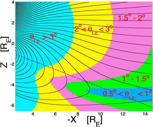
FIGURE 1. The half-angle of the atmospheric loss cone θ_l.c. Is plotted in color. In the light-blue shaded region θ_l.c. > 3^°, in the yellow region 2^° < θ_l.c < 3^°, in the pink shaded region 1.5^° < θ_l.c < 2^°, in the green shaded region 1^° < θ_l.c < 1.5^°, and in the blue shaded region 0.5^° < θ_l.c < 1^°.

Figure 2 shows maps of the magnitude of the loss-cone angular shift eastward in the nightside magnetosphere for electrons of 50 keV (top panel) and 1 MeV (bottom panel). Magnetic-field lines are drawn in black and the Earth’s tilted equatorial plane is denoted by the purple dashed curve. Note that there is a strong “dipole tilt” the with the dipole equator (not marked) southward from the geographic equator on the nightside. The yellow-shaded zones in Figure 2 are regions of the magnetosphere where the atmospheric loss cone angular shift θ_shift is small (< 0.5^°) and the other colors denote regions where the shift θ_shift is stronger (see Figure caption). Comparing the two panels (of Figure 2) it is seen that the shift is larger for 1-MeV electrons than it is for 50-keV electrons: this is because the 1-MeV electrons have larger gyroradii than do the 50-keV electrons. Note in both panels that the loss-cone shift is large where the curvature of the field lines is strong. If anywhere along a field line there is a loss-cone shift θ_shift > 10^°, particles on that field line will undergo field-line-curvature (FLC) scattering (Borovsky et al., 2022a,b) and their orbits will become stochastic. This is because FLC scattering is parameterized by an “adiabaticity parameter” ε = r_gyro/R_c (Il’in et al., 1992; Il’ina et al., 1993), where r_gyro is the gryroradius of the particle with pitch angle 90^° and R_c is the field-line radius of curvature: ε = r_gyro/R_c = 3γmcv_o/eB is related to the loss-cone shift at the equator θ_shift = arcsin (3γmcv/eB), where at small pitch angles ε ≈ θ_shift where θ_shift is measured in radians (cf. Borovsky et al., 2022a). Stochastic behavior onsets when ε ∼ 0.1–0.2 (Birmingham, 1984; Chirikov, 1987; Il’ina et al., 1993), which corresponds to θ_shift ∼ 5.7^°–11.5^°. Note that as ε and θ_shift increase, the onset to stochasticity is slow, not abrupt at particular values of ε and θ_shift (cf. Figure 5 of Borovsky et al., 2022a or Figure 6 of Borovsky et al., 2022b).

FIGURE 2

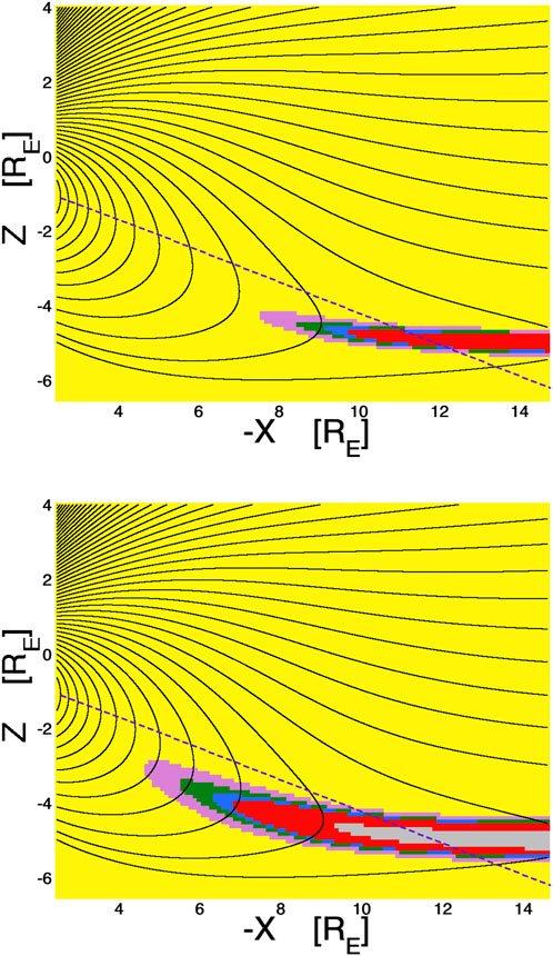
FIGURE 2. Loss-cone-shift maps for electrons. Magnetic-field lines in the nightside magnetosphere in the noon-midnight meridian are drawn as the black curves using the T96 magnetic-field model. The colored shading is the calculated eastward shift of the local atmospheric loss cone for 50-keV electrons (top panel) and for 1-MeV electrons (bottom panels) based on the T96 magnetic-field model. The color scheme is yellow (shift <0.5^°), pink (shift 0.5^°–1^°), green (shift 1^°–1.5^°), blue (shift 1.5^°–2^°), red (shift 2^°–10^°), and gray (shift >10^°).

During other times of the year (away from the December solstice wherein the dipole tilt from the Sun-Earth line is strong) the picture in the nightside magnetosphere is very similar to that depicted in Figure 2. This is demonstrated in Figure 3 where the maps of Figure 2 are recalculated from the T96 model with no dipole tile with respect to the Sun-Earth line. Again, the largest angular shift of the loss cone occurs in the midplane of the plasma sheet where the field-line curvature is strongest.

FIGURE 3

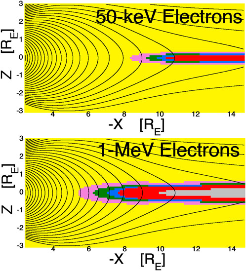
FIGURE 3. Loss-cone-shift maps for electrons as in Figure 2, but for no dipole tilt with respect to the Sun-Earth line. Magnetic-field lines in the nightside magnetosphere in the noon-midnight meridian are drawn as the black curves using the T96 magnetic-field model. The colored shading is the calculated eastward shift of the local atmospheric loss cone for 50-keV electrons (top panel) and for 1-MeV electrons (bottom panels) based on the T96 magnetic-field model. The color scheme is yellow (shift <0.5^°), pink (shift 0.5^°–1^°), green (shift 1^°–1.5^°), blue (shift 1.5^°–2^°), red (shift 2^°–10^°), and gray (shift >10^°).

In Figure 4 two westward-angular-shift maps for protons in the nightside magnetosphere are shown: the top panel is for 10-keV protons (energies typical of the ion plasma sheet) and the bottom panel is for 200-keV protons (energies typical of substorm-injected ions). The gyroradii of protons are in general much greater than the gyroradii of electrons and so the magnitude of the angular shift θ_shift of the loss cone tends to be greater for protons than for electrons. With the loss cone typically being in the range of 3^° or less (cf. Figure 1), one could consider the angular shift of the loss cone to be “significant” if it is 2^° or more. The maps of Figure 4 indicate that the angular shift of the loss cone can be significant (θ_shift > 2^°, red shading) for 200-keV protons at L = 4 and the loss-cone shift can be significant for 10-keV protons at L = 6. The gray shading (θ_shift > 10^°) in the two panels of Figure 4 indicates that one can expect 10-keV protons to have stochastic orbits at L = 8 and 200-keV protons to have stochastic orbits at L = 5 owing to field-line-curvature scattering.

FIGURE 4

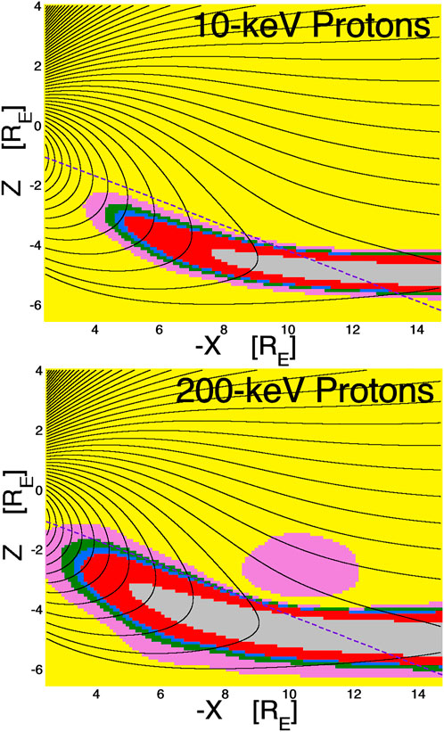
FIGURE 4. Loss-cone-shift maps for protons. Magnetic-field lines in the nightside magnetosphere in the noon-midnight meridian are drawn as the black curves using the T96 magnetic-field model. The colored shading is the calculated eastward shift of the local atmospheric loss cone for 10-keV protons (top panel) and for 100-keV protons (bottom panels) based on the T96 magnetic-field model. The color scheme is yellow (shift <0.5^°), pink (shift 0.5^°–1^°), green (shift 1^°–1.5^°), blue (shift 1.5^°–2^°), red (shift 2^°–10^°), and gray (shift >10^°).

Figure 5 shows two westward-angular-shift maps for oxygen O⁺ in the nightside magnetosphere: the top panel is for 10-keV oxygen (energies typical of the ion plasma sheet) and the bottom panel is for 200-keV oxygen (energies typical of substorm-injected ions). The gyroradii of O⁺ is 4 times the gyroradii of protons at the same kinetic energy and so the angular shift θ_shift of the loss cone tends to be greater for oxygen than for protons. The maps of Figure 5 indicate that the angular shift of the loss cone can be significant (θ_shift > 2^°, red shading) for 200-keV O⁺ at L = 2.5 and the loss cone shift can be significant for 10-keV O⁺ at L = 4. The gray shading (θ_shift > 10^°) in the two panels of Figure 5 indicates that one can expect 10-keV O⁺ to have stochastic orbits at L = 5 and 200-keV O⁺ to have stochastic orbits at L = 4 owing to field-line-curvature scattering.

FIGURE 5

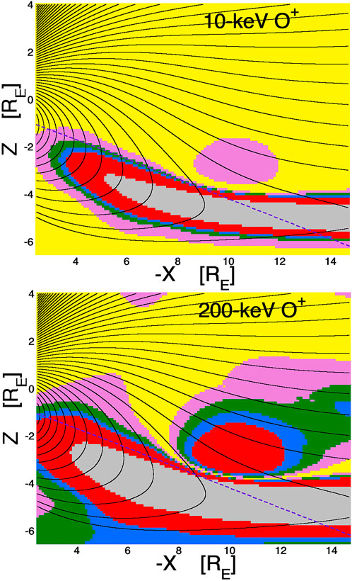
FIGURE 5. Loss-cone-shift maps for oxygen O⁺. Magnetic-field lines in the nightside magnetosphere in the noon-midnight meridian are drawn as the black curves using the T96 magnetic-field model. The colored shading is the calculated westward angular shift of the local atmospheric loss cone for 10-keV O⁺ (top panel) and for 200-keV O⁺ (bottom panels) based on the T96 magnetic-field model. The color scheme is yellow (shift <0.5^°), pink (shift 0.5^°–1^°), green (shift 1^°–1.5^°), blue (shift 1.5^°–2^°), red (shift 2^°–10^°), and gray (shift >10^°).

Using the T96 model for B_z = −5 nT and Dst = −30 nT with no dipole tilt, four loss-cone-shift maps in the equatorial plane of the magnetosphere are plotted in Figure 6. The upper-left panel is the magnitude of the eastward shift for 1-MeV electrons, the upper-right panel is the westward shift for plasma-sheet-energy (10-keV) protons, the lower-left panel is the westward shift for substorm-injection-energy (100-keV) protons, and the lower-right panel is the westward shift for plasma-sheet-energy (10-keV) O⁺ ions. In each panel the Sun is off to the left and the magnetotail is on the right. The yellow shading in each panel represents equatorial regions where the loss-cone shift is minor (<5^°). For the 1-MeV electrons the inner magnetosphere (<5 R_E) exhibits minor shifts, but moving into the transition region and the magnetotail the shift becomes serious. For all four panels of Figure 6 recall that stochastic (finite-larmour-radius) scattering comes in strongly when the loss-cone shift exceeds about 5°, so the red-shaded region marks the transition to stochastic scattering and the gray shaded regions are fully stochastic. For the 10-keV protons (upper-right) the magnitudes of the loss cone shifts are everywhere more serious than they are for the energetic electrons. Even at geosynchronous orbit (6.6 R_E) the shift is serious and stochastic behavior is probably present across the nightside. For the energetic protons and the 10-keV oxygen (bottom two panels) only the very inner magnetosphere would exhibit mild loss-cone shifts and geosynchronous orbit (6.6) would be populated with stochastic orbits. The lower-left panel indicates that what would be commonly called “ring-current” protons at 100-keV may be stochastically scattering in the regions inward of geosynchronous orbit where researchers label the hot ions as ring-current ions.

FIGURE 6

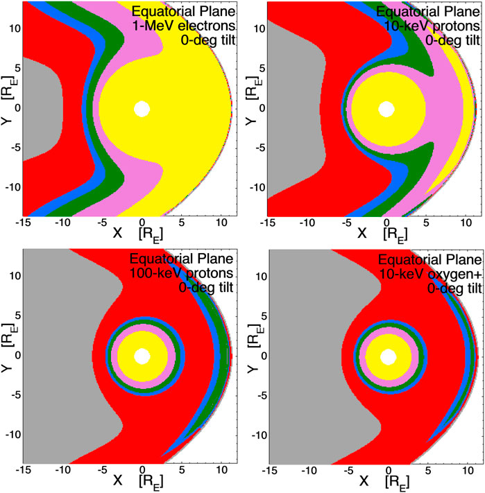
FIGURE 6. Loss-cone-shift maps in the equatorial plane using the T96 magnetc-field model with no dipole tilt. The upper-left is for 1-MeV electrons, the upper right is for 10-keV protons, the lower-left is for 200-keV protons, and the lower-right is for 10-kV oxygen O⁺. The color scheme is yellow (shift <0.5^°), pink (shift 0.5^°–1^°), green (shift 1^°–1.5^°), blue (shift 1.5^°–2^°), red (shift 2^°–10^°), and gray (shift >10^°).

Discussion

A conclusion of the examination of the loss-cone-shift maps is that the angular shift of the loss cone can be important for energetic ions, and even thermal (plasma-sheet) ions throughout the middle and outer magnetosphere and certainly in the magnetotail. Another conclusion is that stochastic scattering via field-line curvature can be important for hot and energetic ions, even in the dipolar portions of the magnetosphere. Hence, ring-current protons and oxygen ions are probably undergoing stochastic scattering. For electrons, important loss-cone shifts and stochastic scattering are limited to the stretched portion of the magnetotail near and beyond the transition region.

Example maps of the magnitude of the loss cone shift for electrons, protons, and oxygen O⁺ ions were created using the T96 (Tsyganenko, 1995; Tsyganenko and Stern, 1996) magnetic-field model with the input parameters B_z = −5 nT for the solar wind and Dst = −30 nT. In the interest of compactness, no parameter variations were performed and no other magnetic-field models were explored. Different magnetic-field models were briefly explored in Sect. 5 of Borovsky et al., 2022b and the different models produce different shift magnitudes (cf. Fig. 9 of Borovsky et al., 2022b).

For future exploration of parameters, the author has a simple-to-use (relativistic) FORTRAN code to efficiently calculate the loss cone shifts for various particle types. The author will make that code available upon request.

Data availability statement

The original contributions presented in the study are included in the article/Supplementary Material; further inquiries can be directed to the corresponding author.

Author contributions

JB initiated this project, performed the numerical orbit calculations, and wrote the manuscript.

Funding

JB was supported at the Space Science Institute by the NSF GEM Program via grant AGS-2027569, by the NASA HERMES Interdisciplinary Science Program via grant 80NSSC21K1406, and by the NASA Heliophysics Mission Concept Studies Program via award 80NSSC22K0113.

Acknowledgments

The author thanks Gian Luca Delzanno and Kateryna Yakymenko for helpful conversations.

Conflict of interest

The authors declare that the research was conducted in the absence of any commercial or financial relationships that could be construed as a potential conflict of interest.

Publisher’s note

All claims expressed in this article are solely those of the authors and do not necessarily represent those of their affiliated organizations, or those of the publisher, the editors and the reviewers. Any product that may be evaluated in this article, or claim that may be made by its manufacturer, is not guaranteed or endorsed by the publisher.

References

Birmingham, T. J. (1984). Pitch angle diffusion in the Jovian magnetodisc. J. Geophys. Res. 89, 2699–2707. doi:10.1029/ja089ia05p02699

CrossRef Full Text | Google Scholar

Borovsky, J. E., Delzanno, G. L., Dors, E. E., Thomsen, M. F., Sanchez, E. R., Henderson, M. G., et al. (2020a). Solving the auroral-arc-generator question by using an electron beam to unambiguously connect critical magnetospheric measurements to auroral images. J. Atmos. Sol. Terr. Phys. 206, 105310. doi:10.1016/j.jastp.2020.105310

CrossRef Full Text | Google Scholar

Borovsky, J. E., Delzanno, G. L., and Henderson, M. G. (2020b). A mission concept to determine the magnetospheric causes of aurora. Front. Astron. Space Sci. 7, 595292. doi:10.3389/fspas.2020.595929

CrossRef Full Text | Google Scholar

Borovsky, J. E., Delzanno, G. L., and Yakymenkno, K. N. (2022a). Pitch-angle diffusion in the Earth’s magnetosphere organized by the Mozer-transformed coordinate system. Front. Astron. Space Sci. 9, 810792. doi:10.3389/fspas.2022.810792

CrossRef Full Text | Google Scholar

Borovsky, J. E., Yakymenkno, K. N., and Delzanno, G. L. (2022b). Modification of the loss cone for energetic particles in the Earth’s inner magnetosphere. J. Geophys. Res. 123, e2021JA030106. doi:10.1029/2021JA030106

CrossRef Full Text | Google Scholar

Chirikov, B. V. (1987). Particle confinement and adiabatic invariance. Proc. Roy. Soc. Lond. A 413, 145–156.

Google Scholar

Il’in, V. D., Kuznetsov, S. N., Yushkov, B. Y., and Il’in, I. V. (1992). Quasiadiabatic model of charged-particle motion in a dipole magnetic confinement system under conditions of dynamic chaos. JETP Lett. 55, 645–649.

Google Scholar

Il’ina, N., Il’in, V. D., Kuznetsov, S. N., Ysushkov, B. Y., Amirkhanov, I. V., and Il’in, I. V. (1993). Model of nonadiablatic charged particle mostion in the field of a magnetic dipols. JETP 77, 246–252.

Google Scholar

Mozer, F. S. (1966). Proton trajectories in the radiation belts. J. Geophys. Res. 71, 2701–2708. doi:10.1029/jz071i011p02701

CrossRef Full Text | Google Scholar

Porazik, P., Johnson, J. R., Kaganovich, I., and Sanchez, E. (2014). Modification of the loss cone for energetic particles. Geophys. Res. Lett. 41, 8107–8113. doi:10.1002/2014gl061869

CrossRef Full Text | Google Scholar

Powis, A. T., Porazik, P., Greklek-Mckeon, M., Amin, K., Shaw, D., Kaganovich, I. D., et al. (2019). Evolution of a relativistic electron beam for tracing magnetospheric field lines. Front. Astron. Space Sci. 6, 69. doi:10.3389/fspas.2019.00069

CrossRef Full Text | Google Scholar

Roederer, J. G., and Zhang, H. (2014). Dynamics of magnetically trapped particles. Berlin: Springer-Verlag.

Google Scholar

Sanchez, E. R., Powis, A. T., Kagonovich, I. D., Marshall, R., Porazik, P., Johnson, J., et al. (2019). Relativistic particle beams as a resource to solve outstanding problems in Space Physics. Front. Astron. Space Sci. 6, 71. doi:10.3389/fspas.2019.00071

CrossRef Full Text | Google Scholar

Tsyganenko, N. A. (1995). Modeling the Earth's magnetospheric magnetic field confined within a realistic magnetopause. J. Geophys. Res. 100, 5599. doi:10.1029/94ja03193

CrossRef Full Text | Google Scholar

Tsyganenko, N. A., and Stern, D. P. (1996). Modeling the global magnetic field of the large-scale Birkeland current systems. J. Geophys. Res. 101, 27187–27198. doi:10.1029/96ja02735

CrossRef Full Text | Google Scholar

Willard, J. M., Johnson, J. R., Snelling, J. M., Powis, A. T., Kaganovich, I. D., and Sanchez, E. R. (2019). Effect of field-line curvature on the ionospheric accessibility of relativistic electron beam experiments. Front. Astron. Space Sci. 6, 56. doi:10.3389/fspas.2019.00056

CrossRef Full Text | Google Scholar