A selective up-sampling method applied upon unbalanced data for flare prediction: potential to improve model performance

1 Introduction

Flare prediction plays an important role in space weather forecast. The photospheric magnetic field information of active regions (ARs) is valuable (Yu et al., 2009), and the data are helpful in accurately predicting solar flares, which can be extended up to less than 10 days before the eruption (Alipour et al., 2019). The solar flare might be accompanied by the coronal mass ejection (CME). Furthermore, CMEs might impact the Earth and affect the geospace such as by triggering geomagnetic storms, causing damage to the electricity transmission system (Quebec Blackout event in 1989 (Boteler, 2019)) and disabling the space satellite equipment.

Many photospheric magnetic parameters of ARs are highly related to strong-flare occurrences, for example, SHARP (Spaceweather HMI Active Region Patch) parameters, which are available from the data product called Spaceweather HMI Active Region Patches (Bobra et al., 2014), given by the Helioseismic and Magnetic Imager (HMI) onboard the Solar Dynamics Observatory (SDO).

Solar observations are used in different situations, such as the HMI photospheric line-of-sight magnetic field and multi-wavelength EUV filtergrams (Jarolim et al., 2022), SHARP parameters (Zhang et al., 2022), critical scales of parameters under the κ-scheme (Kusano et al., 2020), and HMI magnetograms (Bobra and Couvidat, 2015), for predicting solar flares under different conditions. Dhuri et al. (2019) showed that the SHARP parameters are the leading contributors to the machine classification, so we decided to use the SHARP parameters in the following experiments for flare prediction as our initial research direction.

In recent years, machine learning algorithms have been applied to solar physics and have made progress in flare prediction, especially in extracting new predictors and developing effective models (Liu et al., 2017; Wang et al., 2020; Chen et al., 2022; Sun et al., 2022; Wang et al., 2022; Li et al., 2022; Nishizuka et al., 2021; Sun et al., 2021). Liu et al. (2017) adopted the random forest method for the multiclass classification of flares. Wang et al. (2020) adopted the long short-term memory (LSTM) network to learn from the time series of magnetic parameters. Sun et al. (2022) adopted a stacking ensemble approach to combine the convolutional neural network (CNN) and LSTM. Wang et al. (2022) extracted the predictor MSE, the mean squared errors between the pictures of the ARs and the corresponding reconstructed pictures derived by an unsupervised auto-encoder network, from the radial magnetic field of SHARPs. Li et al. (2022) adopted the knowledge-informed CNN/fusion model to develop a classification model to predict the strong flares in the next 48 h. Furthermore, Nishizuka et al. (2021) developed the Deep Flare Net with an operable interface to detect ARs, extract their features, and conduct a prediction of the probability of flares within 24 h. Furthermore, Sun et al. (2021) expanded their machine learning method to the interpretability of its neural network.

As we all know, strong flares are rare events, which leads to an unbalanced dataset consisting of a relatively small number of positive samples (referred to as strong-flare events) and a large number of negative samples (referred to as non-strong-flare events). Prediction models trained by an unbalanced dataset might be sensitive to the bias and achieve limited performance at last. Therefore, how to balance positive and negative samples in the dataset for flare prediction is considered one of the difficult and crucial problems to tackle.

There are some widely used methods tackling unbalanced data in machine learning, for example, the Synthetic Minority Over-sampling Technique (SMOTE) up-sampling method (Chawla et al., 2002), which is used to establish a balanced dataset by increasing the number of minority samples; a random down-sampling method (Japkowicz, 2000), which is used to randomly remove samples from a majority to create a balanced dataset; and the weighted-class method (Hashemi and Karimi, 2018), which is used to eliminate the bias of the model that was trained on the unbalanced dataset by enlarging the weight of low-probability categories.

However, the question arises whether those widely used methods can be well applied to our dataset for flare prediction and provide good results. On the one hand, randomly increasing the positive samples might lead to too much noise and make the generated samples away from the ground truth. On the other hand, decreasing the negative samples will lead to a loss of a lot of valid information. If we increase the number of positive samples selectively considering the correlation between the flare occurrence and magnetic parameters of ARs, will it help us obtain a better classification model that is more accurate and more reliable?

In this study, we focused on tackling the unbalanced dataset for flare prediction and developed a selective up-sampling method by picking up more positive samples from the mixed-up region (referred to as the confusing distribution areas consisting of both the positive and negative samples). Then, we conducted a comparable analysis of the influence of the input dataset on model performance.

The remainder of the paper is organized as follows: data preparation is given in Section 2. In section 3, we introduce the selective up-sampling method and develop a strong-flare prediction model. Then, we conduct a comparable analysis of the model performance based on different input datasets in Section 4. The conclusion and discussion are given in Section 5.

2 Data preparation

The dataset was obtained from the Helioseismic and Magnetic Imager data product on the Solar Dynamics Observatory, which is called SHARPs.

The SHARP parameters, including 16 photospheric magnetic parameters, such as the total magnetic flux, spatial gradients of the field, characteristics of the vertical current density, current helicity, and a proxy for the integrated free magnetic energy (Bobra et al., 2014), were calculated per patch and were available on a 12-min cadence. Furthermore, SHARP parameters have been widely used to develop flare prediction models by statistical and machine learning methods (Sinha et al., 2022) because many previous studies showed that these parameters play an important role in characterizing the properties and complexity of ARs (Leka and Barnes, 2003; Georgoulis and Rust, 2007).

Active area parameters were stored in each SHARP series as keywords (Bobra et al., 2014), and the data we used in this paper were sampled from the hmi.sharp_720s dataset, verified by Huang et al. (2018), and published on Alibaba Tianchi. The dataset contained 10 photospheric magnetic parameters, whose correlation coefficient matrix was calculated and is shown in Figure 1 with a thermal heatmap. The meaning of photospheric magnetic parameters has been described in detail by Bobra et al. (2014), and we listed a brief description and formula of six keywords of the parameters that have the greatest correlation with strong flares in each activity area of the dataset in Table 1.

FIGURE 1

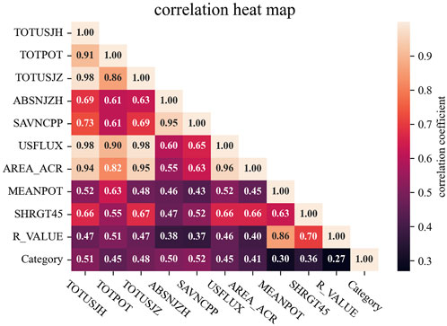
FIGURE 1. Correlation coefficient matrix heatmap of photospheric magnetic parameters and event categories.

TABLE 1

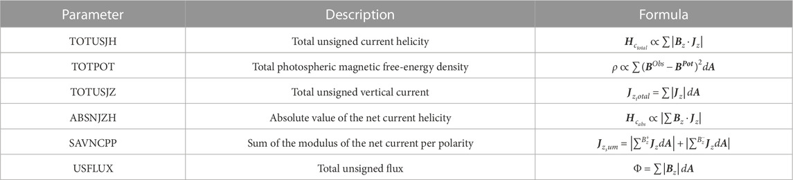
TABLE 1. Keywords for six active-region parameters in the SHARP series.

The strong-flare events (positive samples) included at least one flare of the M and above class within 48 h. The non-strong-flare events (negative samples) included no flares or only flares of the C and below class. In this study, we focused on strong-flare events because they are highly related to the geoeffectiveness.

For the flare forecasting task, Ahmadzadeh et al. (2021) suggested some rules on normalization, class imbalance, temporal coherence, performance metrics, and comparison of models. In this study, we adopted the data normalization method for data preprocessing, proposed a selective up-sampling method considering class imbalance and temporal coherence for model training, and used an evaluation metrics (F1 score that should be less biased through class imbalance) for model evaluation.

Furthermore, the rules for selecting data for this dataset are as follows:

(1) The time range is from 16:00 on 4 May 2010 to 16:00 on 26 January 2019.

(2) The time interval for sampling the same event is 96 min (the sampling frequency is lower than that of the SDO) in order to guarantee enough variations between the closest AR images.

(3) The location range of SHARPs is within ±30 heliolongitude degrees from the solar disk center to reduce the influence of projection. Cui et al. (2007) evaluated this issue of the influence of the AR projection effect on the solar flare productivity and found that the projection effect can be ignored for ARs located within ±30° from the solar disk center.

First, we need to divide the training set and testing set in a scientific way. The rules are as follows:

(1) The ratio of positive to negative samples should be similar in both training and testing sets. This has two purposes. First, to avoid the situation where the number of positive examples in the testing set is too small or even zero (very likely to occur if the datasets are divided randomly). Second, as the proportion of positive cases in the testing set is close to that in reality, the testing results can reflect the real performance of the model when facing the actual situation.

(2) The data in the training and testing set cannot be from the same event, which is to ensure that the testing and training sets are independent of each other, and active regions with multiple flares cannot appear in both training and testing sets simultaneously (Dhuri et al., 2019).

In this study, we used only the photospheric magnetic parameter data that contain 73,810 samples (from 2,542 ARs) of photospheric magnetic parameters. After the statistics, we found that there were only 2,988 positive samples from 155 strong-flare ARs (the climate probability ≈ only 6%) and the remaining 70,822 samples from 2,387 non-strong-flare ARs were all negative, which makes it extremely difficult for machine learning methods to predict flares only through these original and imbalanced data because the classifier can easily learn the information of the majority of non-strong-flare events, but there are not enough strong-flare events to learn from.

In each round of experiments, we divided the dataset into the training set and the testing set randomly in a 9:1 ratio. At the same time, in both training and testing sets, we ensured that the ratio of positive to negative samples is approximately the same. Furthermore, we ensured that the data in the testing set and the training set come from different ARs for data independence.

3 Application of processing methods upon unbalanced data for flare prediction

In order to eliminate the negative impact of data imbalance, there are some ways that are widely used in industrial applications, which will also be used as control groups in the following data training in this study:

(1) Random down-sampling method: Random sampling from the majority samples (negative samples, as for flare prediction) to make its number equal to the minority samples (positive samples, as for flare prediction).

(2) SMOTE up-sampling method (Chawla et al., 2002): We took one dataset from the minority samples (positive samples) and named it x_i, calculated and sorted it according to the Euclidean distance between this sample and other samples, and then took the first n samples (n is the sampling multiple number set according to the sample imbalance ratio) as the selected nearest neighbors $\widehat{x_{i1}},\widehat{x_{i2}},\dots ,\widehat{x_{in}}$. Furthermore, for each $\widehat{x_{ij}}$, we constructed a new sample x_new according to the following formula:

$x_{new}=x_i+rand\left(\mathrm{0,1}\right)\cdot \left(\widehat{x_{ij}}-x_i\right)$

(3) Weighted classifier: This did not change the samples but changed the weights corresponding to different categories in the classifier. When there are mixed samples, the classifier will be more inclined to retain more minority samples.

The three photospheric magnetic parameters that have the greatest correlations with the strong-flare occurrence were selected for this study, namely, the total unsigned current helicity (TOTUSJH), the absolute value of net current helicity (ABSNJZH), and the sum of the modulus of the net current per polarity (SAVNCPP).

The frequency densities of the photospheric magnetic parameter in positive and negative samples are shown in Figure 2A (taking TOTUSJH as an example), and the number distribution is shown in Figure 2B. The statistical characteristics indicate that when the values of these photospheric magnetic parameters are low, positive samples are totally submerged by negative samples; on the contrary, when the parameter values are high, almost all samples are positive. It means that on the one hand, when creating new samples while up-sampling in this region, a large number of negative samples are likely to be classified as positive samples, thus seriously losing the accuracy of the model; while, on the other hand, when the parameter values are large, there are only positive samples, so it is unnecessary to up-sample the positive samples here for the model to learn more. However, there is a mixed-up region referred to as the confusing distribution areas consisting of both strong-flare events and non-strong-flare events (as marked in Figure 2B). The mixed-up region can be quantitatively described as the region near the strong-flare probability of 50%. Here, the strong-flare probability is the probability of a strong flare occurring within 48 h. In the mixed-up regions, the number of positive samples and negative samples is similar, so the characteristics are the most difficult to distinguish. We assumed that it is worthwhile to up-sample the positive examples in these mixed-up regions and proposed the selective up-sampling method.

FIGURE 2

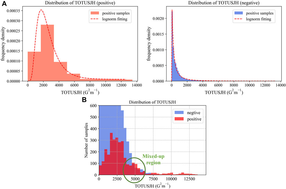
FIGURE 2. Distribution of the photospheric magnetic parameter (taking TOTUSJH as an example). The Y-axis in (A) represents the frequency density, and the Y-axis in (B) represents the number of samples at different intervals (since the negative samples are far more than the positive samples, the range of Y only considers the positive sample to show the details). The green circular box indicates the mixed-up region of the two types of samples.

3.1 Probability function of flare occurrences based on SHARP parameters

As we need a convincing method to identify the mixed-up regions for the selective up-sampling method, it is necessary to know the quantitative relationship between strong-flare probability and photospheric magnetic parameters. We can see that the photospheric magnetic parameters in strong-flare events and non-strong-flare events both show the characteristics of a skewed distribution, which can be fitted with the standard form of log-normal function as follows:

$f\left(x\right)=lognorm\left(x,\sigma \right)=\frac{1}{xlna\sqrt{2\pi }\sigma }{e}^{-\frac{{\left({\mathit{log}}_{a}x\right)}^2}{2{\sigma }^2}},a=eforthestandardform.(1)$

The aforementioned formula represents the probability density of the photospheric magnetic parameter when its value is x, which has different σ values in positive and negative samples.

Furthermore, when the form of the probability density of photospheric magnetic parameters in positive samples and that in negative cases are known, we can derive the form of the probability function of strong-flare occurrence (P_f) based on Bayes’ theorem as follows (Barnes and Leka, 2008):

Bayes’ theorem can be used to estimate the probability of a flare occurring event. When the magnetic parameter is equal to x, the probability of a strong flare occurring within 48 h is equal to

$P\left(strong|x\right)=\frac{P\left(x|strong\right)\cdot P\left(strong\right)}{P\left(x|strong\right)\cdot P\left(strong\right)+P\left(x|notstrong\right)\cdot P\left(notstrong\right)}(2)$

Since P (x|strong) and P (x|not strong) → 0, through L’Hôpital’s rule, we can obtain

$P\left(strong|x\right)=\frac{f\left(x|strong\right)\cdot P\left(strong\right)}{f\left(x|strong\right)\cdot P\left(strong\right)+f\left(x|notstrong\right)\cdot P\left(notstrong\right)}(3)$

By replacing f with Eq 1, P (class) with N (class)/N (total), we can make the probability function of strong flare P (strong|x) as a function of P_f with x as the input and two sigma parameters as tuning parameters:

$P_f\left(x,{\sigma }_1,{\sigma }_0\right)=\frac{lognorm\left(x,{\sigma }_1\right)\cdot N_1}{lognorm\left(x,{\sigma }_1\right)\cdot N_1+lognorm\left(x,{\sigma }_0\right)\cdot N_0}(4)$

This indicates the probability of strong flares when the photospheric magnetic parameter value is x, where σ₁ and σ₀ representing the standard deviation of lnx in positive samples and negative samples, respectively, are the parameters we need to fit. Moreover, N₁ and N₀ are the number of positive samples and negative samples, respectively.

We can fit the observed strong-flare probability to the probability function as previously mentioned. Dividing the photospheric magnetic parameter into 16 bins according to Doane’s rule (Doane, 1976), the proportion of positive samples in each interval p_i can be used as the probability data to be fitted. By assuming each interval as a separate sample population estimated to be normally distributed, the Wilson confidence intervals (Wilson, 1927) in each interval can be written as follows (Figure 3)

$\left({\omega }_i^{-},{\omega }_i^{+}\right)\equiv \frac{p_i+z^2/2n\pm z\sqrt{p_i\left(1-p_i\right)/n_i+z^2/4n_i^2}}{1+z^2/n_i}$

FIGURE 3

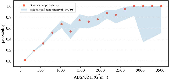
FIGURE 3. Wilson confidence intervals under different photospheric magnetic parameter values. The observation probability and its confidence intervals at different intervals containing different sample numbers are shown.

Here, n_i represents the number of samples in the ith interval and z = 1.96 under the 95% confidence interval. The advantage of using the Wilson confidence intervals is that it can show confidence intervals for any sample size without making specific assumptions about the sample size. In addition, the method can also effectively solve the deviation problem in binomial distribution parameter estimation, thus improving the accuracy of the confidence interval.

In order to accelerate the convergence speed of fitting, we scaled the input x. The values of the two sigma parameters in Eq. 4 and scaling factor α (which means that the input value of the function is αx) in fitting graphs of three different photospheric magnetic parameters (Figure 4) are as follows: for TOTUSJH (G²m⁻¹), the best fitting parameters are σ₁ = 3158.18, σ₀ = 1.53, and α = 0.23; for ABSNJZH (G²m⁻¹), the best fitting parameters are σ₁ = 33.53, σ₀ = 1.89, and α = 0.85; and for SAVNCPP (A), the best fitting parameters are σ₁ = 44.28, σ₀ = 1.96, and α = 2.94e − 11.

FIGURE 4

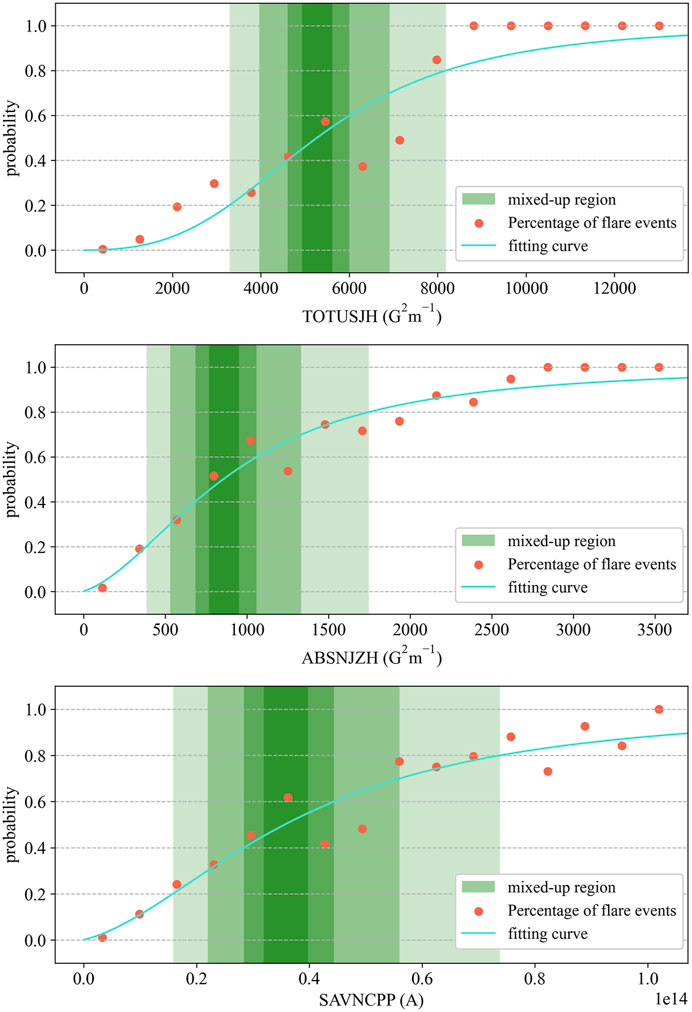
FIGURE 4. Fitting curve of the flare occurrence probability and the mixed-up region division. The mixed-up regions are selected near the flare yield of 50%. The green parts are the mixed-up regions divided based on three photospheric magnetic parameters (TOTUSJH, ABSNJZH, and SAVNCPP), and the depth of their colors represents different probability ranges: 50±5%, 50%±10%, 50%±20%, and 50%±30% (from deep to light).

After fitting the functional relationship between the strong-flare probability and the photospheric magnetic parameters, we divided four mix-up regions according to the fitting curve with “p = 50%” as the median line: 50±5%, 50%±10%, 50%±20%, 50%±30%, as shown in detail in Figure 4. Furthermore, the selective up-sampling method applied to low-probability positive samples in these regions can then be realized.

3.2 Flare prediction model based on sampling methods

The training information including the control groups is as follows:

(1) Raw data group: The original unbalanced data are directly sent to the logical regression model, which contains 56,869 negative samples, 2,837 positive samples, and 66,428 samples in total.

(2) Random down-sampling group: After the down-sampling, 2,837 negative samples, 2,837 positive samples, and 5,674 samples in total are sent to the logical regression model.

(3) SMOTE up-sampling group: After the up-sampling, 56,869 negative samples, 56,869 positive samples, and 1,13,738 samples in total are sent to the logical regression model.

(4) Weighted classifier: The input data are not changed, but the weight of different categories in the classifier is changed according to the number of samples. In this training set, the ratio of majority samples to minority samples is 20, so the weight of the minority category (strong flare) should be 20 times that of the majority samples (non-strong flare). The input data of the model contain 56,869 negative samples, 2,837 positive samples, and 66,428 samples in total.

(5) Selective up-sampling group: We determine the mixed-up regions through the method introduced in the previous section and expand the positive samples by repeating them in the mix-up region until it has size as same as the negative samples. The input data from the first round of experiments contain 56,869 negative samples, 56,869 positive samples, and 1,13,738 samples in total.

We obtained the parameter distributions before and after resampling, as shown in Figure 5 (we take TOTUSJH as an example). The KL divergence value of strong-flare events before and after sampling was calculated as follows: KL (random down-sampling) = 0; KL (SMOTE up-sampling) = 0.02; and KL (selective up-sampling) = 1.70. It can be seen that the selective up-sampling method has the greatest impact on the parameter distribution of strong-flare events.

FIGURE 5

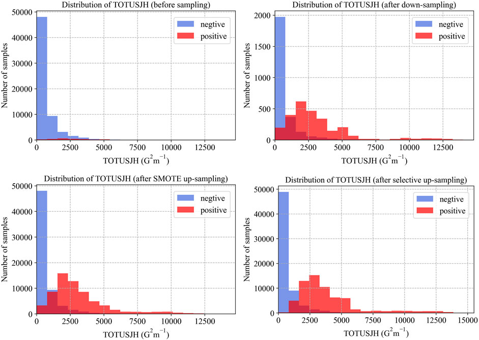
FIGURE 5. Parameter distribution before and after resampling (taking TOTUSJH as an example). The four images show the distribution before sampling, after down-sampling, SMOTE up-sampling, and selective up-sampling.

Furthermore, for each newborn sample, we added a random perturbation (±5%) to each value separately, as small random differences can improve the performance of the model. The reason of not using the SMOTE method is that the distribution of the newborn samples supplemented by the SMOTE method may be quite different from the original minority samples, which will weaken the characteristics of this region where we need to strengthen the recognition, but the method in Section 3.2 (5) will not have this negative effect.

After feeding the data to each logistic regression model, the logistic regression algorithm will adjust the model parameters through the gradient descent method to reduce the cross entropy loss round by round until it reaches a certain threshold (we set it at 0.001), as a sign of the end of training.

The models in different groups are tested on the same testing set and we give the evaluation results in Section 4, while evaluation indicators are introduced in Section 3.3.

3.3 Evaluation metrics

For a binary classification task like flare prediction, the confusion matrix is listed in Table 2. The true positive (TP) is the hit case, where the strong-flare events are correctly classified in the strong-flare category. The false positive (FP) is the false alarm case, where the non-strong-flare events are falsely classified as the strong-flare category. The false negative (FN) is the miss case, where strong-flare events are falsely classified as the non-strong-flare category. The true negative (TN) is the correct negative sample, where the non-strong-flare samples are correctly classified as the non-strong-flare category.

TABLE 2

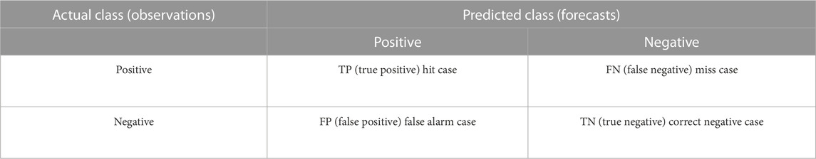
TABLE 2. Confusion matrix for binary classification.

Based on the confusion matrix, we adopted three evaluation metrics: recall, precision, and F1 score, which are computed as follows:

$recall=\frac{TP}{TP+FN}$

$precision=\frac{TP}{TP+FP}$

$F1=\frac{2\times precision\times recall}{precision+recall}$

Because the samples are unbalanced, and we only focus on the prediction of samples with flares, we do not need to calculate the evaluation results of negative samples and the accuracy of positive samples. (In fact, they are all close to 1 because of data imbalance). The scikit-learn package (https://scikit-learn.org) is used to calculate the aforementioned metrics.

4 Comparison analysis of model performance

For such flare data samples, due to the imbalance of data, we chose not to consider the accuracy rate because its results are greatly affected by TN, and as the number of negative samples is large, the effect of training on negative samples (non-strong-flare events) is good, which makes the accuracy of the model close to 1 at any time. Thus, the recall and precision references are compared for their model performance.

After 10 rounds of random experiments, the evaluation results of the same logistic regression model sampled in different ways are shown in Figure 6. The mean and standard deviation of the results are listed in Table 3.

FIGURE 6

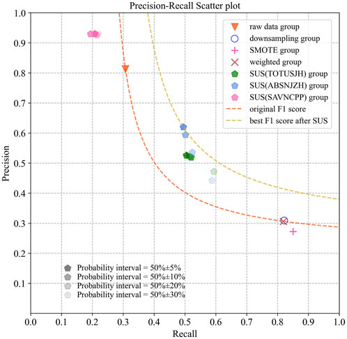
FIGURE 6. Model testing results, where SUS refers to the method of selective up-sampling. The dotted line represents the equivalent curve of the F1 score. The more the curve deviates to the upper right, the greater the value of the F1 score is. We can find that most of the results of the selective up-sampling method on mixed-up regions are better than those of the original data and other sampling methods. (The dark-yellow dotted line represents the best result of the F1 score sampled in the mixed-up regions, while the orange dotted line represents the result of training the raw data without sampling. Furthermore, the color depth of the point represents the width selected for the sampling region near the strong-flare yield of 50%).

TABLE 3

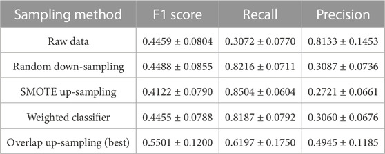
TABLE 3. Prediction results of the model on the testing dataset (average ± standard deviation).

It can be found that although the precision of the models trained on the original data is high, the recall is extremely low (about 0.3). On the contrary, after SMOTE up-sampling, random down-sampling, or training using a weighted classifier, although the recall is improved, the precision is seriously reduced at the same time (from 0.8 to 0.3).

By up-sampling the positive samples related to strong-flare events in the mixed-up region before training, the best F1 score reaches 0.5501 ± 0.1200, which is approximately 22−33% higher than other methods. In this simple comparison, we can draw the conclusion that the performance of the model significantly improved.

The reason for the improvement is that the categories of events cannot be distinguished by a certain photospheric magnetic parameter in its mixed-up region. Therefore, the classifier may lose a dimension of information in this region. By repeatedly up-sampling minority samples in the mixed-up region, we can strengthen the information here for the classifier. Furthermore, by adding some random disturbances, we not only avoid over fitting but also make newborn data close to the real situation.

5 Conclusion and discussion

In this study, we focused on tackling the unbalanced dataset based on SHARP parameters. After repeatedly up-sampling the minority samples in the mixed-up region and adding some random disturbances, we compared their model performances. The methods used in the comparison are as follows: 1) raw data (no processing); 2) random down-sampling; 3) SMOTE up-sampling; and 4) weighted classifier; which are all described in detail in Section 3. Furthermore, the result shows that the forecast capability is promoted in the mixed-up region, the robustness of the model is increased, and the selective up-sampling method has potential to improve the model performance in strong-flare prediction as its F1 score reaches 0.5501 ± 0.1200, which is approximately 22−33% higher than the other methods.

The purpose of increasing the number of samples from the mixed-up region of positive strong-flare samples (selective up-sampling) is to better distinguish the previous “difficult to predict” events. Furthermore, the method of adding samples is based on the original samples plus random values, which is close to the ground truth, while it is likely that the created physical parameter values might deviate significantly from the ground truth if we use SMOTE or other up-sampling methods. The selective up-sampling method we proposed could provide a new suggestion on the preparation of data for the machine learning model in the future, especially when we expand data for unbalanced samples.

This study also presents the characteristics of interdisciplinary. On the one hand, the application modeling of the AI method is valuable, while on the other hand, it also requires manual improvements based on data characteristics rather than simply using it directly.

Although the proposed sampling method reaches a higher F1 score than the other three sampling methods, it is consistent with the other existing methods. The main reason is that in this experiment we developed a flare forecasting model based on only three parameters adopting a relatively simple algorithm (logistic regression) for classification. In this study, we highlighted the importance of the sampling method tackling the class-imbalance problem. We found that the selective up-sampling method has potential to improve the flare forecasting performance. Considering that many complex machine learning models can help boost the model performance significantly compared to simple statistical models, in the future, we would like to adopt other models (for example, CNN + LSTM) and investigate comparable studies on flare forecasting.

Moreover, as the time resolution of SHARP data is high enough (sampling every 12 min), timing information of continuous samples will be used as well, which will increase the amount of information contained in the photospheric magnetic parameters by another dimension, so as to assist solar-flare forecast better. We are currently working on applying this method for combining continuous magnetograms and photospheric magnetic parameters with the time dimension.

Data availability statement

The original contributions presented in the study are included in the article/Supplementary Material; further inquiries can be directed to the corresponding author.

Author contributions

SL, JW, YC, ML, JG, YS, BL, and SL meet the authorship criteria and agree to be accountable for the content of the work. All authors contributed to the article and approved the submitted version.

Funding

JW was supported by the National Science Foundation of China (Grant No. 42074224), the Youth Innovation Promotion Association, CAS, the Key Research Program of the Chinese Academy of Sciences (Grant No. ZDRE-KT-2021-3), and Pandeng Program of National Space Science Center, Chinese Academy of Sciences.

Acknowledgments

The authors thank the SDO/HMI team members that contributed to the SDO mission. They also thank the reviewers for providing valuable suggestions.

Conflict of interest

The authors declare that the research was conducted in the absence of any commercial or financial relationships that could be construed as a potential conflict of interest.

Publisher’s note

All claims expressed in this article are solely those of the authors and do not necessarily represent those of their affiliated organizations, or those of the publisher, the editors, and the reviewers. Any product that may be evaluated in this article, or claim that may be made by its manufacturer, is not guaranteed or endorsed by the publisher.

References

Ahmadzadeh, A., Aydin, B., Georgoulis, M. K., Kempton, D. J., Mahajan, S. S., and Angryk, R. A. (2021). How to train your flare prediction model: Revisiting robust sampling of rare events. Astrophysical J. Suppl. Ser.254, 23. doi:10.3847/1538-4365/abec88

CrossRef Full Text | Google Scholar

Alipour, N., Mohammadi, F., and Safari, H. (2019). Prediction of flares within 10 days before they occur on the sun. Astrophysical J. Suppl. Ser.243, 20. doi:10.3847/1538-4365/ab289b

CrossRef Full Text | Google Scholar

Barnes, G., and Leka, K. (2008). Evaluating the performance of solar flare forecasting methods. Astrophysical J.688, L107–L110. doi:10.1086/595550

CrossRef Full Text | Google Scholar

Bobra, M. G., and Couvidat, S. (2015). Solar flare prediction using sdo/hmi vector magnetic field data with a machine-learning algorithm. Astrophysical J.798, 135. doi:10.1088/0004-637x/798/2/135

CrossRef Full Text | Google Scholar

Bobra, M. G., Sun, X., Hoeksema, J. T., Turmon, M., Liu, Y., Hayashi, K., et al. (2014). The helioseismic and magnetic imager (hmi) vector magnetic field pipeline: Sharps - space-weather hmi active region patches. doi:10.1007/s11207-014-0529-3

CrossRef Full Text | Google Scholar

Boteler, D. (2019). A 21st century view of the march 1989 magnetic storm. Space weather.17, 1427–1441. doi:10.1029/2019SW002278

CrossRef Full Text | Google Scholar

Chawla, N. V., Bowyer, K. W., Hall, L. O., and Kegelmeyer, W. P. (2002). Smote: Synthetic minority over-sampling technique. J. Artif. Intell. Res.16, 321–357. doi:10.1613/jair.953

CrossRef Full Text | Google Scholar

Chen, J., Li, W., Li, S., Chen, H., Zhao, X., Peng, J., et al. (2022). Two-stage solar flare forecasting based on convolutional neural networks. Space Sci. Technol.2022. doi:10.34133/2022/9761567

CrossRef Full Text | Google Scholar

Cui, Y., Li, R., Wang, H., and He, H. (2007). Correlation between solar flare productivity and photospheric magnetic field properties ii. magnetic gradient and magnetic shear. Sol. Phys.242, 1–8. doi:10.1007/s11207-007-0369-5

CrossRef Full Text | Google Scholar

Dhuri, D. B., Hanasoge, S. M., and Cheung, M. C. (2019). Machine learning reveals systematic accumulation of electric current in lead-up to solar flares. Proc. Natl. Acad. Sci.116, 11141–11146. doi:10.1073/pnas.1820244116

PubMed Abstract | CrossRef Full Text | Google Scholar

Doane, D. P. (1976). Aesthetic frequency classifications. Am. Statistician30, 181–183. doi:10.1080/00031305.1976.10479172

CrossRef Full Text | Google Scholar

Georgoulis, M. K., and Rust, D. M. (2007). Quantitative forecasting of major solar flares. Astrophysical J.661, L109–L112. doi:10.1086/518718

CrossRef Full Text | Google Scholar

Hashemi, M., and Karimi, H. (2018). Weighted machine learning. Statistics, Optim. Inf. Comput.6, 497–525. doi:10.19139/soic.v6i4.479

CrossRef Full Text | Google Scholar

Huang, X., Wang, H., Xu, L., Liu, J., Li, R., and Dai, X. (2018). Deep learning based solar flare forecasting model. i. results for line-of-sight magnetograms. Astrophysical J.856, 7. doi:10.3847/1538-4357/aaae00

CrossRef Full Text | Google Scholar

Japkowicz, N. (2000). “Learning from imbalanced data sets: A comparison of various strategies,” in AAAI workshop on learning from imbalanced data sets (AAAI Press Menlo Park, CA), 68, 10–15. Available at: https://www.aaai.org/Papers/Workshops/2000/WS-00-05/WS00-05-003.pdf.

Google Scholar

Jarolim, R., Veronig, A., Podladchikova, T., Thalmann, J., Narnhofer, D., Hofinger, M., et al. (2022). Interpretable solar flare prediction with deep learning. Tech. Rep. Copernic. Meet. doi:10.5194/egusphere-egu22-2994

CrossRef Full Text | Google Scholar

Kusano, K., Iju, T., Bamba, Y., and Inoue, S. (2020). A physics-based method that can predict imminent large solar flares. Science369, 587–591. doi:10.1126/science.aaz2511

PubMed Abstract | CrossRef Full Text | Google Scholar

Leka, K., and Barnes, G. (2003). Photospheric magnetic field properties of flaring versus flare-quiet active regions. ii. discriminant analysis. Astrophysical J.595, 1296–1306. doi:10.1086/377512

CrossRef Full Text | Google Scholar

Li, M., Cui, Y., Luo, B., Ao, X., Liu, S., Wang, J., et al. (2022). Knowledge-informed deep neural networks for solar flare forecasting. Space weather.20. doi:10.1029/2021SW002985

CrossRef Full Text | Google Scholar

Liu, C., Deng, N., Wang, J. T., and Wang, H. (2017). Predicting solar flares using sdo/hmi vector magnetic data products and the random forest algorithm. Astrophysical J.843, 104. doi:10.3847/1538-4357/aa789b

CrossRef Full Text | Google Scholar

Nishizuka, N., Kubo, Y., Sugiura, K., Den, M., and Ishii, M. (2021). Operational solar flare prediction model using deep flare net. Earth, Planets Space73, 64–12. doi:10.1186/s40623-021-01381-9

CrossRef Full Text | Google Scholar

Sinha, S., Gupta, O., Singh, V., Lekshmi, B., Nandy, D., Mitra, D., et al. (2022). A comparative analysis of machine learning models for solar flare forecasting: Identifying high performing active region flare indicators, 05910. arXiv preprint arXiv:2204. doi:10.3847/1538-4357/ac7955

CrossRef Full Text | Google Scholar

Sun, H., Manchester IV, W., and Chen, Y. (2021). Improved and interpretable solar flare predictions with spatial and topological features of the polarity inversion line masked magnetograms. Space weather.19, e2021SW002837. doi:10.1029/2021SW002837

CrossRef Full Text | Google Scholar

Sun, Z., Bobra, M. G., Wang, X., Wang, Y., Sun, H., Gombosi, T., et al. (2022). Predicting solar flares using cnn and lstm on two solar cycles of active region data. Astrophysical J.931, 163. doi:10.3847/1538-4357/ac64a6

CrossRef Full Text | Google Scholar

Wang, J., Luo, B., and Liu, S. (2022). Precursor identification for strong flares based on anomaly detection algorithm. Front. Astronomy Space Sci.300. doi:10.3389/fspas.2022.1037863

CrossRef Full Text | Google Scholar

Wang, X., Chen, Y., Toth, G., Manchester, W. B., Gombosi, T. I., Hero, A. O., et al. (2020). Predicting solar flares with machine learning: Investigating solar cycle dependence. Astrophysical J.895, 3. doi:10.3847/1538-4357/ab89ac

CrossRef Full Text | Google Scholar

Wilson, E. B. (1927). Probable inference, the law of succession, and statistical inference. J. Am. Stat. Assoc.22, 209–212. doi:10.1080/01621459.1927.10502953

CrossRef Full Text | Google Scholar

Yu, D., Huang, X., Wang, H., and Cui, Y. (2009). Short-term solar flare prediction using a sequential supervised learning method. Sol. Phys.255, 91–105. doi:10.1007/s11207-009-9318-9

CrossRef Full Text | Google Scholar

Zhang, H., Li, Q., Yang, Y., Jing, J., Wang, J. T., Wang, H., et al. (2022). Solar flare index prediction using sdo/hmi vector magnetic data products with statistical and machine learning methods. arXiv preprint arXiv:2209.13779. Available at: https://arxiv.org/abs/2209.13779.

Google Scholar