PINE-RT: An operational real-time plasmasphere model

1 Introduction

The plasmasphere is a region of cold $(\sim 1eV)$ and dense (up to $\sim 10^{4}c{m}^{-3}$) plasma around the Earth. A sharp drop in the density defines its outer boundary, which is called the plasmapause. The source of plasmaspheric particles is the ionosphere and its size and shape can vary dramatically under the influence of the solar wind. During quiet geomagnetic conditions, it has a toroidal shape extending for several Earth radii into space, corotating with the Earth. Instead, during geomagnetic storms the plasmasphere shrinks considerably as the plasma is dragged towards the Sun, and sunward elongated structures, called plumes, appear, e.g., (Goldstein et al., 2003a; Spasojević et al., 2003). During the recovery phase of a storm, the plasmasphere is refilled with particles from the ionosphere untill it reaches the toroidal shape and size of quiet geomagnetic conditions.

Several processes are influenced by the plasmasphere, as for example, the GPS navigation (Mazzella and Andrew, 2009; Xiong et al., 2016), the surface charging of the satellites (Reeves et al., 2013) and the propagation and growth of plasma waves which in turn affect the distributions of energetic ions and electrons in radiation belts through wave-particle interaction (Horne et al., 2005; Orlova et al., 2016; Shprits et al., 2016). In particular, the plasmapause location separates different regions of hiss- and chorus-wave-induced scattering (Shprits et al., 2008; Li and Hudson, 2019). Therefore, the modeling of the plasmasphere is crucial both for space weather applications and as a scientific topic per se.

There has been a long history of research in plasmasphere modelling. Early attempts consisted in developing empirical models of the plasma density using statistical averages (Carpenter and Anderson, 1992; Sheeley et al., 2001). The plasma density was inferred from plasma-wave measurements from spacecrafts (Carpenter and Anderson, 1992) and satellite (Sheeley et al., 2001) missions and from ground-based whistler measurements (Carpenter and Anderson, 1992). These models provide an accurate description of the plasma density during quiet conditions and are still extensively used in space-physics simulations, but they cannot describe the dynamics during disturbed geomagnetic conditions (Zhelavskaya et al., 2017; Shprits et al., 2022).

More recently, machine-learning models have been developed in order to connect more closely the plasma density with the geomagnetic conditions (Bortnik et al., 2016; Chu X. et al., 2017; Chu X. N. et al., 2017; Zhelavskaya et al., 2017; Zhelavskaya et al., 2021). These models are based on feedforward neural networks (Haykin, 1994; Hassoun, 1995), which are machine learning models able to capture non-linear relations between the inputs and the target. The plasma density has been inferred from spacecraft potential (Bortnik et al., 2016; Chu X. et al., 2017) and plasma-wave measurements (Chu X. N. et al., 2017; Zhelavskaya et al., 2017; Zhelavskaya et al., 2021). In particular (Zhelavskaya et al., 2017; Zhelavskaya et al., 2021), developed the PINE (Plasma density in the Inner magnetosphere Neural network-based Empirical) model, describing the plasma density in the equatorial plane (Zhelavskaya et al., 2017) performed a long-term validation of the PINE model using in situ plasma density data inferred from the plasma-wave measurements of the Van Allen Probes (Mauk et al., 2013). Moreover they compared the global plasmaspheric reconstructions of the PINE model to the plasmapause locations extracted from the images provided by the IMAGE EUV instrument (Sandel et al., 2000) for selected events. They found that the PINE model is able to reproduce the plasma erosion, the plasmapause location, the plumes and their rotation during quiet geomagnetic conditions and moderate storms. Despite the remarkable success, the machine-learning models face the difficulty to describe accurately what happens during strong geomagnetic storms, because these are rare events for which much less data is available (Zhelavskaya et al., 2017; Zhelavskaya et al., 2021).

There has also been extensive effort in developing physics-based models, see e.g., (Bailey et al., 1997; Pierrard et al., 2008; Pierrard and Stegen, 2008; Huba and Krall, 2013; Krall and Huba, 2013; Ridley et al., 2014; Huba et al., 2017; Zhelavskaya et al., 2021; Haas et al., 2023) and (Pierrard et al., 2009) for a review. These models describe the physical processes with dynamical equations, relying on parameters estimated empirically via statistical averages. These parameters include the refilling-rates from the ionosphere and the electric and magnetic fields driving the plasma dynamics. In particular (Zhelavskaya et al., 2021), adopted the Versatile Electron Radiation Belt Convection-Simplified (VERB-CS) model, which was originally developed by (Aseev and Shprits, 2019) to model the low energy electrons of the radiation belts (Zhelavskaya et al., 2021) extensively compared the predictions of the VERB-CS model to the PINE model results and showed that the VERB-CS model describes the plasma dynamics better than the PINE model during strong geomagnetic storms, but the PINE model is more accurate during quiet conditions and moderate geomagnetic storms.

The Prediction of Adverse effects of Geomagnetic storms and Energetic Radiation (PAGER) project 1 aims at estimating the risks of satellite charging1 2 days ahead in order to enable satellite operators to respond to events that represent a significant threat. Moreover, it provides several space-weather-forecasts products that are made available in real-time through its website. The backbone of the PAGER project is constituted by a pipeline of algorithms connecting the solar activity with the satellite charging. A crucial component of this pipeline is dedicated to forecast the plasma density in the plasmasphere in the equatorial plane and the plasmapause location. Having the objective of providing the forecasts 1–2 days ahead, a possible way to provide the plasma density forecast would be to have a nowcast machine-learning model whose inputs can be forecasted 1–2 days ahead. We note that the PINE model can not be used in this respect, because it requires the geomagnetic indices AE, Kp, Sym-H, and F10.7, the magnetic-shell parameter L and the magnetic local time (MLT) as inputs, but the forecasts of AE, Sym-H, and F10.7 are not provided by the PAGER components. Instead there are PAGER components forecasting the Kp index and the solar wind properties at the L1 Lagrange point.

In this study, we report the detailed derivation of a nowcast machine-learning model of the plasma density in the equatorial plane having only the Kp index and solar wind properties as inputs. We call this model PINE-RT as it has been inspired by the PINE model and it has been developed to run in real-time (RT). We extensively validated the PINE-RT model and compared its predictions with the predictions of the VERB-CS and the PINE models. In order to evaluate the performance of the models, we made use of the in situ plasma density inferred from the plasma-wave measurements of the Van Allen Probes and the plasmapause locations extracted from the images of the IMAGE EUV instrument. We explored both the Volland-Stern electric field model (Volland, 1973; Stern, 1975) as in (Zhelavskaya et al., 2021) and the Weimer (Weimer, 2005) electric field model as inputs for the VERB-CS model. We chose to consider events characterized by quiet conditions or moderate disturbances while the modeling of strong geomagnetic storms is deferred to future studies. In fact strong storms (Kp > 7) are rarer events and appropriate procedures must be tailored to enable the machine-learning algorithms to accurately describe them (Zhelavskaya et al., 2017; Zhelavskaya et al., 2021). We found that our machine-learning model has a performance slightly inferior to the one of the PINE model and slightly better than the VERB-CS model driven by the Volland-Stern electric field model, while the VERB-CS model driven by the Weimer electric field model gives the worst performance. We implemented the PINE-RT model to run in real-time and its output is available on the PAGER project website and throught the iSWA service of the Community Coordinated Modeling Center2.

We describe the derivation of the PINE-RT model and the VERB-CS model in Section 2. In Section 3 we show the validation and the comparison of our machine-learning model with the VERB-CS and the PINE models. Finally, we summarize our findings and we point to ideas for future studies in Section 4.

2 Materials and methods

2.1 The PINE-RT model

2.1.1 Data

Following (Zhelavskaya et al., 2017; Zhelavskaya et al., 2021), we used the in situ plasma density inferred from the upper-hybrid-resonance frequency bands in the dynamic spectrograms of the Electric and Magnetic Field Instrument Suite and Integrated Science (EMFISIS) instrument (Kletzing et al., 2013) on board the Van Allen Probes with the Neural-network-based Upper hybrid Resonance Determination (NURD) algorithm (Zhelavskaya et al., 2016). This data is provided by the German Research Centre for Geosciences (GFZ) (Zhelavskaya et al., 2020). We also made use of the Kp index provided by the GFZ (Matzka et al., 2021) and of the solar-wind measurements at the L1 Lagrange point provided by the OMNIWeb service3. We collected all the data for the period 01 October 2012—01 July 2016.

We divided the data into 6 parts, we used 5 of these to perform the 5-fold cross validation for model selection, see Subsection 2.1.4, and one for testing the selected model. We partitioned the data by randomly assigning blocks of 35 sequential days to one of the 6 parts. There are three reasons for this (Zhelavskaya et al., 2021). First, the data points are temporally correlated and a completely random split may lead to a correlation between the training and the test data points, potentially leading to an optimistic estimation of the performance on the test dataset. Second, a sequential split encompassing large time periods may lead to a significantly different distribution of the features and the target variable in the training and in the test datasets. For example, due to the way the data is split, it may occur that the training or the test datasets do not contain periods of high geomagnetic activity. Finally, the reason for using 35-day blocks is to avoid the possible effect of the 27-day recurrence caused by the solar rotation.

2.1.2 Feature engineering

In (Zhelavskaya et al., 2021) a machine-learning model based only on solar wind features achieved a lower performance than a model based on geomagnetic indices or on a combination of solar wind and geomagnetic indices. Therefore, we decided to look primarly for a model that has both the solar wind features and the Kp index as input, but we also checked the performance of models having only solar wind features as input (see Section 2.1.4). Moreover, we decided to focus our attention in particular on features that were shown to be relevant for the description of the plasmasphere. In particular, the Kp index and vB_s, where v is the solar wind speed and B_s is the southward component of the interplanetary magnetic field (IMF), were found to be important for the plasmapause dynamics (He et al., 2017). For this reason, we decided to include these features. Finally, we also included the proton density ρ_p, since it is an important property of the solar wind.

We computed aggregates of Kp, vB_s and ρ_p over the time windows in Table 1 in order to take into account the effect of their time history. In particular, we computed the maximum value for Kp and the mean for vB_s and ρ_p.We note that the time windows were chosen to be non-overlapping in order to avoid the creation of correlated features. Moreover, the time windows were selected differently for the features due to their different cadency. In particular, the Kp index has a 3-h cadency, so aggregates below this temporal window do not make sense, while the solar wind features have a 1-min cadency to capture the short-term dynamics.

TABLE 1

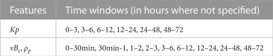
TABLE 1. Time windows considered to capture the effect of the time history of Kp, vB_s and ρ_p on the plasma density dynamics.

The solar wind features may have missing values, which most often occurs during geomagnetic storms. When computing the aggregates, we required at least 30% of the values to be present in a given window. If that minimum percentage was not reached, we assigned a NaN value to the aggregate. The machine-learning algorithm cannot be fitted on those data points for which the values of some features are missing. Therefore, one would need either to find a strategy to fill the missing values or to exclude those data points from the training dataset. Since the strategy for filling the missing values would require a separate study, we decided to exclude the data points with missing values from the training dataset.

We considered up to 72-h time history in order to take into account the plasmasphere refilling which happens on a time scale of several days (Craig et al., 1993). We checked the perfomance of models taking into account either up to 48-h or up to 72-h time history (see Section 2.1.4).

Finally, we considered L and MLT to parametrize the equatorial plane. Instead of providing MLT as input to the machine-learning models, we employed sin (MLT) and cos (MLT) to provide the information that MLT is an angular variable.

2.1.3 Features scaling

When developing a machine-learning algorithm, it is generally recommended to have all the features on the same order of magnitude. This is why we applied a scaling procedure tailored to the distributions of the features and chose to obtain values between 0 and 1. L takes values between 1 and 6.5 (it is measured in Earth radii), while sin (MLT) and cos (MLT), which ranges from −1 and 1. Then we scaled these features with the MinMax scaler4, which applies the following transformation to the features values x_scaled = (x − x_min)/(x_max − x_min) and makes the values to be between 0 and 1. In Figure 1 we report the histograms of the Kp index and of the mean of ρ_p and vB_s over the last-three-hours period, since the aggregates of the features over the other time windows show a similar behaviour. The histograms are computed using 4 of the 5 folds composing the training data in order not to extract information from the validation data.

FIGURE 1

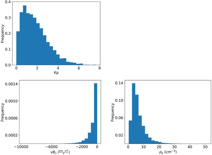
FIGURE 1. Distributions of the Kp index and of the mean of ρ_p and vB_s over the last 3 hours computed using 4 of the 5 folds composing the training set.

We notice that the Kp index is distributed between 0 and 8, with the majority of values being below 3. Then, we scaled the Kp-related features with the MinMax scaler, bringing the values of the features between 0 and 1. The last-three-hours mean of ρ_p has values greater than 0 and lower than 70, with the majority of values being below 20, and shows a quite light tail. For this reason, we scaled the density-related features by first applying a logarithmic transformation in natural base. Since the resulting distributions looked gaussian-like we applied a standard scaler5 making the distribution to have 0 mean and a variance of 1. Finally, we applied a MinMax scaler, making the values of the features to be between 0 and 1. The last-three-hours mean of vB_s takes values from roughly −12,000 and 0, with the majority of values being above −4,000, and shows a lighter tail than the ρ-related features. Moreover, it takes negative values and also 0. For these reasons, we first multiplied the vB_s-related features by −1 and shifted by 1, then we took the logarithm in base 10 and finally we applied the MinMax scaler.

Both the standard scaler and MinMax scaler have parameters that need to be computed during the training process of the machine-learning model. For the standard scaler one has to fit compute the mean and the variance of the feature values, while for the MinMax scaler has to compute the minimum and the maximum value of the feature values. Once these parameters have been computed during the training process, the scaling transformations can be applied both to the training data and to new unseen data.

In Figure 2 we show the distributions of the features considered in Figure 1 after applying the scaling procedure. We notice that all the features have value between 0 and 1 after the scaling. Moreover when looking at the scaled distribution of the last-three hours mean of vB_s, we can clearly distinguish the cases in which the magnetic field was positive or negative on average.

FIGURE 2

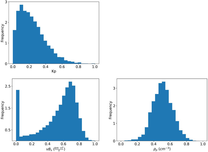
FIGURE 2. Scaled distributions of the Kp index and of the mean of ρ_p and vB_s over the last 3 hours using 4 of the 5 folds composing the training set.

2.1.4 Features selection and model selection

Starting from the features described in Section 2.1.2, we looked for the best features set among those defined in Table 2.To do this, we evaluated the performance of the features sets as inputs of the machine-machine learning model we intended to use to model the plasma density, which is a feedforward neural network.

TABLE 2

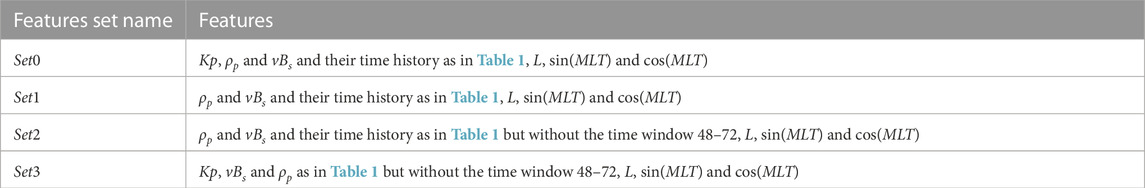
TABLE 2. The features sets for which we evaluated the performance.

A feedforward neural network (Haykin, 1994; Hassoun, 1995) is a neural network wherein connections between the nodes do not form a cycle. It is constituted by an input layer, one or more hidden layers and an output layer, with several neurons in each layer. In a given layer, each neuron receives inputs from the neurons of the previous layer and gives an output to the neurons of the next layer. Interestingly, feedforward neural networks are able to capture non-linear relations between the features and the target, and they were successfully used in space physics (Bortnik et al., 2016; Zhelavskaya et al., 2016; Chu X. et al., 2017; Zhelavskaya et al., 2017; Zhelavskaya et al., 2021). In particular (Zhelavskaya et al., 2017), showed that a feedforward neural network with one hidden layer is able to accurately predict the plasma density in the equatorial plane of the plasmasphere. Therefore we chose to select our model within this class of models.

We considered 7, 15, 20, 25, and 30 as possible choices for the numbers of neurons in the hidden layer. To evaluate which architecture performs best, we performed a 5-fold cross validation using the 5 datasets contained in the training dataset. K-fold cross validation is used for model selection, because it avoids the choose a model on the basis of its performance on a particular dataset (Zhelavskaya et al., 2017, 2021). In this procedure the training dataset is split in K-folds, where one fold is considered as the validation dataset and the remaining ones are used as training dataset to train the model. We notice that the training concerns all the parts of the model that need to be fixed, i.e., also the scalers described in Subsection 2.1.3. The performance is evaluated both on the training and validation datasets. This procedure is repeated for all the K-possibilities providing K performance values on the training and the validation datasets, from which statistical quantities can be computed.

In our case, we have 5 folds and therefore 5 couples of training and validation datasets on which we computed the performance. In particular, we used the root mean squared error (RMSE), which is defined as

$RMSE=\sqrt{\frac{\sum _{i=1}^N{\left(n_{i,true}-n_{i,pred}\right)}^2}{N}},(1)$

where n_i,true and n_i,pred are the log₁₀ of the plasma density data extracted with the NURD algorithm and of the plasma density predicted by the neural network for the i-data point, respectively. N is the total number of data points for which we predicted within a given dataset. In Figure 3, we show the mean and the standard deviation of the RMSEs obtained during the 5-fold cross validation for the features Set0. One can see that the RMSE on the training dataset reduces as we increase the number of neurons, which is expected since the model becomes more complex and is able to fit better to the training data. Instead the RMSE on the validation dataset first decreases and then starts to oscillate after 15 neurons. In machine learning, it is expected that there is a gap between the performance on the training and on the validation dataset, since the algorithm is fitted on the training dataset. However, when that gap increases as the complexity of the model increases, it means that the model starts to specialize more to the training data and has not the same prediction power on unseen data. In our case, the gap between the RMSE on the training and the validation dataset increases when the number of neurons is above 15, we then chose to have 15 neurons in the hidden layer and this fixed the model.

FIGURE 3

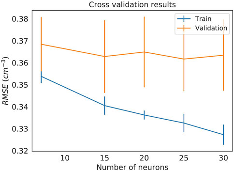
FIGURE 3. Plot of the mean and standard deviation of the RMSE derived from the cross validation procedure for the features set 0.

We have performed this procedure for each features set in Table 2 and we report the best results obtained in Table 3. We can see that the features sets with only solar wind features achieve a lower performance than the ones containing also the Kp index, similarly to what was found in (Zhelavskaya et al., 2021). Moreover, the features Set 0, which uses up to 72-h of time history, performs slightly better than Set 3 containing up to 48-h of time history. For these reasons, we adopted the features Set 0 and a hidden layer with 15 neurons, which gave the best result with Set 0.

TABLE 3

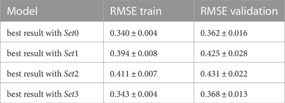
TABLE 3. Best results obtained for the features sets of Table 2.

2.1.5 Performance on the test dataset and final model

We evaluated the performance of the model selected in Section 2.1.4 on the test dataset, which was not part of the training data. To do this, we fitted the scalers defined in Subsection 2.1.3 and the model Section 2.1.4 on the whole training dataset and we computed the RMSE both on the training and the test datasets. We found RMSE = 0.34 on the training data and RMSE = 0.35 on the test data, which is compatible with the cross validation results of Table 3.

In order to obtain the final PINE-RT model, we combined the training and the test data and we retrained our scalers and neural-network model using both datasets. The neural-network model has a random_state parameter, which determines the random initialization of the weights and the bias parameters of the model6. These are the parameters of the neural-network that are fitted during the training process. While training the final model, we fixed the random_state to eliminate the randomness from the training process of the neural network and ensure the reproducibility of the model. We present the extensive validation of the PINE-RT model in Section 3, where we also compare its performance with the one of the VERB-CS model of Section 2.2.

2.1.6 Implementation of the real-time runs

We deployed the PINE-RT model described in Section 2.1.5 to run in real-time. The input data for the real-time runs are downloaded or generated by the PAGER components. In particular, we combine the real-time solar-wind measurements at L1 provided by the ACE spacecraft7, which are regularly downloaded on the PAGER servers, with the solar wind forecasted by the SWIFT code8. As for the Kp index, we combine several sources. First, we use the Kp index measurements provided by GFZ (Matzka et al., 2021), which is downloaded on the PAGER servers. Second, we use two forecasts of the Kp index, that are generated in the context of the PAGER project. One forecast is based on the algorithm of (Shprits et al., 2019) and is driven by the solar-wind measurements at L1. The other forecast is obtained by providing the solar-wind forecast of SWIFT to the Kp nowcast algorithm of (Shprits et al., 2019). Finally, we make use of the Kp index forecast provided by the Space Weather Prediction Center9 as a backup solution. The real-time plots of the Kp index sources available in PAGER can be found here10.

The PINE-RT model runs every hour and predicts the next-day forecast of the plasma density in the equatorial plane and the plasmapause location with 1-h cadency. A movie of the output is publicly available on the PAGER website11 and the nowcast is also available throught the iSWA service of the Community Coordinated Modeling Center12. Finally the PINE-RT model runs in a Docker container13 to ensure cross-platform portability and resilience, the latter in light of a possible future integration with Kubernetes14.

2.2 The VERB-CS model

During active geomagnetic periods, Birkland currents (Stern, 1983) will form, which cause a strong dawn-to-dusk electric field. This field transports particles from the plasma sheet across the inner magnetosphere towards the magnetopause on the dayside. Such trajectories are known as open-drift shells. If the co-rotational electric field, which is seen by an observer outside the co-rotational inertial reference frame of the Earth, is strong enough to close this trajectory before the particles encounter the magnetopause, particles will be trapped. Depending on the spatial location, the particles will either be on a closed or an open drift path (see Figure 4). The outermost closed drift path of zero energy particles assuming static electric and magnetic fields is known as the Alfvén layer. As a zero-order approximation, the Alfvén layer roughly predicts the plasmapause location.

FIGURE 4

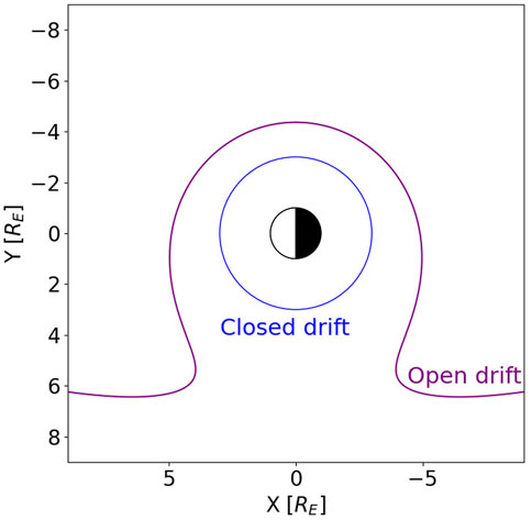
FIGURE 4. Schematic comparison between electrons on open and closed drift paths.

The physics-based model describing convection and refilling from the ionosphere is based on the Versatile Electron Radiation Belt (VERB) model, which is capable of simulating the electron population within the Earth’s radiation belts (Shprits et al., 2008; Subbotin and Shprits, 2009; Subbotin et al., 2011) in three dimensions and electron ring current population in four dimensions (Shprits et al., 2015; Aseev and Shprits, 2019) by describing the particles in a convective-diffusive manner (Schulz and Lanzerotti, 1974). Low energy electrons are dominated by the convective transport, making it possible to neglect the diffusion terms, resulting in the VERB-CS (Convection Simplified) model (Aseev and Shprits, 2019)

$\frac{\partial n_e}{\partial t}+v_{\mathrm{\Phi }}\frac{\partial n_e}{\partial \mathrm{\Phi }}+v_R\frac{\partial n_e}{\partial R}=S-L.(2)$

The VERB-CS model has been previously used to model the plasma density n_e in the plasmasphere in the equatorial plane (Zhelavskaya et al., 2021) by solving Equation 2, where Φ is the magnetic local time (MLT), R is the radial distance from the Earth in the equatorial plane, v_Φ and v_R are drift velocities respectively in MLT and radial distance, S represents the source and L the loss of charged particles. Good results during geomagnetic storms have been reported in (Zhelavskaya et al., 2021) by driving the convection with the Volland-Stern electric field model (Volland, 1973; Stern, 1975) in combination with a sub-auroral polarization stream (SAPS) module (Goldstein et al., 2005). For the full model description, we refer to Zhelavskaya et al. (2021), as the model used in our study only deviates in the electric and magnetic fields driving convection. Instead of using the simple dipole approximation to describe the ambient magnetic field as in Zhelavskaya et al. (2021), we use the Kp-dependent T89 magnetic field model (Tsyganenko, 1989), since the dipole approximation does not hold at large radial distances, especially during geomagnetic disturbed times (Tsyganenko, 1989). It should be noted that the T89 model overestimates the magnetic field, but it is relatively easy to implement as it uses only the Kp index as an input. Regarding the ambient electric field, we use the Volland-Stern model parameterized by Kp (Chen et al., 1975; Maynard and Chen, 1975) using a gamma factor of 1.8 (Zhelavskaya et al., 2021) and including the SAPS module (Goldstein et al., 2005). Additionally, we report results using the Weimer electric field model Weimer (2005), which takes solar wind parameters as input and calculates the polar cap potential, which is mapped along magnetic field lines down to the equatorial plane. Afterwards, the electric field is calculated at the equatorial plane numerically using a central differencing scheme. Solar wind parameters are binned to 15-min intervals and fed to the Weimer model, resulting in a much higher time resolution compared to the 3-h cadence of the Volland-Stern model. As a result, the Weimer model promises to describe finer and quicker changes of the shape and strength of the convection electric field.

3 Results

Here we show the results of the validation of the PINE-RT model and its comparison with the VERB-CS and the PINE models. In order to compare the models, we considered the predictions of the models for the same events. We performed a long-term comparison using the equatorial plasma density inferred with the NURD algorithm from the Van Allen Probe RBSP-A in situ data. To perform an unbiased evaluation, this was done using data which were not included in the training dataset of the machine-learning model. Moreover, we evaluated the global plasmapheric reconstructions of the models on selected events using the plasmapause extracted from the images of the IMAGE EUV instrument (Sandel et al., 2000). We consider events related to quiet conditions and moderate geomagnetic storms characterized by Kp < = 7, postponing the evaluation of the models on strong storms with Kp > 7 to future work.

We used the Kp index provided by GFZ (Matzka et al., 2021) and the solar wind measurements at L1 and the geomagnetic indices for the PINE model from OMNIWeb15. The features for the PINE-RT model were constructed with the same procedure as in Subsection 2.1.2 and scaled as in Subsection 2.1.3 with the scalers fitted in Subsection 2.1.5.

3.1 Validation with Van Allen Probes data

We chose to consider the equatorial plasma density inferred from the Van Allen Probe RBSP A data for the period 1 September 2016–1 May 2017, which was not included in the training dataset of the machine-learning model. We generated the predictions of the VERB-CS and the machine-learning models on a spatio-temporal grid of L, MLT and time. In fact VERB-CS has it is own grid which does not exactly match the locations of the RBSP-A observations in L, MLT, and time. For the machine learning models we make predictions on the VERB-CS grid to be able to easily compare with the physics-based models. The spatial grid was between 1.5 and 6.5 Earth radii at steps of 0.25 Earth radii and between 0 and 24 at steps of 0.5 for MLT, while we had a 15 min resolution in time. The predictions of all the models are then lineary interpolated in L, MLT and time to match the L-, MLT- and time-coordinates of the RBSP-A observations.

In Figure 5 we show the predictions of the models and the equatorial plasma density extracted from the RBSP-A data with the NURD algorithm. In Figures 6, 7 we show respectively the absolute logarithmic differences and the logarithimic differences between the predictions of the models and the equatorial plasma density data. Finally, in Figure 8 we plot the histograms of the logarithmic differences and we report the RMSE and mean error (ME) of the predictions. We notice that the PINE model has the best performance both in terms of RMSE and ME, followed by the PINE-RT model which outperforms the VERB-CS model driven by the Volland-Stern electric field in terms of RMSE. Finally, the VERB-CS model driven by the Weimer electric field gives the worst performance both in terms of RMSE and ME. Looking at the ME, we notice that the models have a tendency to underestimate the density, which is more pronounced for the model driven by the Weimer electric field. Interestingly, looking at Figure 5 we qualitatively see that the VERB-CS model tends to underestimates the density for L < 4, while in this region the machine-learning models appears to be less biased. Finally, the machine-learning models have the most gaussian-like distributions of the errors, as it can be seen in Figure 8.

FIGURE 5

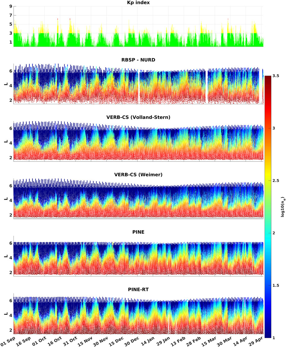
FIGURE 5. In the top panel we plot the Kp index for the period 1 September 2016–1 May 2017. In the other panels, we report the predictions of the machine-learning and physics-based models and the equatorial plasma density, extracted from RBSP-A data with the NURD algorithm (Zhelavskaya et al., 2016), using a log10 logarithmic scale.

FIGURE 6

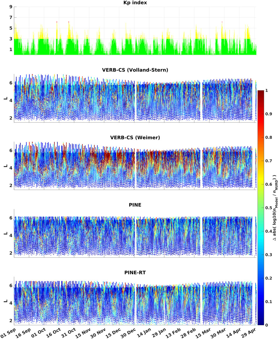
FIGURE 6. In the top panel we plot the Kp index for the period 1 September 2016–1 May 2017. In the other panels, we report the absolute logarithmic differences between the predictions of the machine-learning and physics-based models and the equatorial plasma density extracted from the RBSP-A data with the NURD algorithm (Zhelavskaya et al., 2016).

FIGURE 7

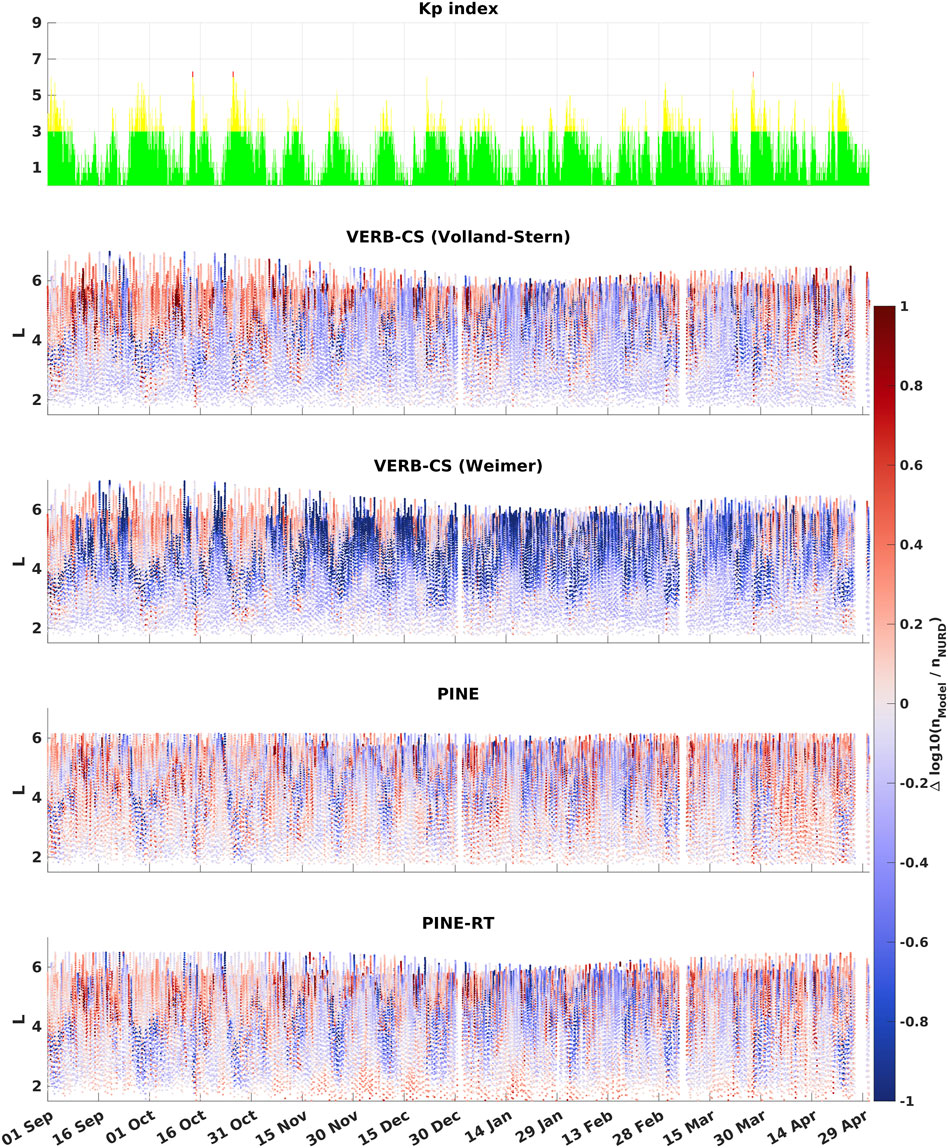
FIGURE 7. In the top panel we plot the Kp index for the period 1 September 2016–1 May 2017. In the other panels, we report the logarithmic differences between the predictions of the machine-learning and physics-based models and the equatorial plasma density extracted from the RBSP-A data with the NURD algorithm (Zhelavskaya et al., 2016).

FIGURE 8

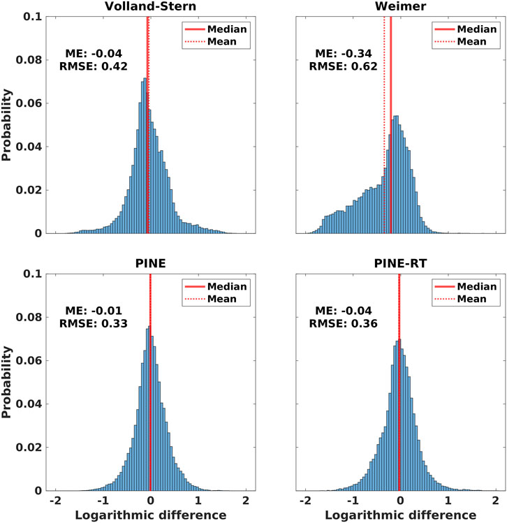
FIGURE 8. We report the histograms of the logarithmic differences between the predictions of the machine-learning and physics-based models and the equatorial plasma density data inferred from the RBSP-A data with the NURD algorithm (Zhelavskaya et al., 2016) for the period 1 September 2016–1 May 2017.

In order to have a closer look into the comparison between the predictions of the models and the observations, we show the predictions of the models and the equatorial plasma density extracted from the RBSP-A data with the NURD algorithm for the period 17 April 2017–24 April 2017 in Figure 9. This period is characterized by quiet times and moderate geomagnetic disturbances as one can see from the Kp index. We notice that all the models reproduce quite well the observations.

FIGURE 9

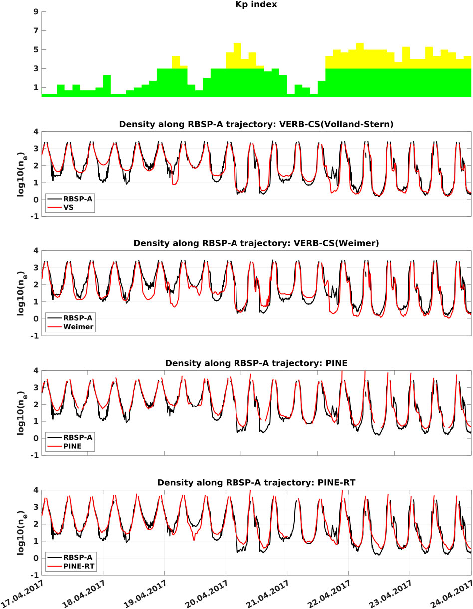
FIGURE 9. In the top panel we plot the Kp index for the period 17 April 2017–24 April 2017. In the other panels, we report the predictions of the machine-learning and physics-based models and the equatorial plasma density, extracted from RBSP-A data with the NURD algorithm (Zhelavskaya et al., 2016), using a log10 logarithmic scale.

3.2 Validation with Image EUV data

In addition to compare with the equatorial plasma density inferred from the Van Allen Probes data, it is important to check the consistency of the global plasmapheric predicted by our models. The images produced by the IMAGE EUV instrument (Sandel et al., 2000) on board of the IMAGE mission16 show the He⁺ distribution in the plasmasphere (Goldstein et al., 2003b) showed that the sharp edges in the IMAGE EUV images coincide with the actual plasmapause locations. This fact makes the IMAGE EUV images unique in providing insights into the global plasmaspheric dynamics, see e.g., (Goldstein et al., 2003a; Spasojević et al., 2003).

The IMAGE mission operated during a different solar cycle than the one we used while training the machine-learning model. Therefore we consider the IMAGE EUV images one of the best sources of data available to validate the consistency of the global plasmaspheric reconstructions of our models. We compare the plasmapause predictions of the models against the plasmapause locations manually extracted from the IMAGE EUV images and provided by17, which is based on the method developed in (Goldstein et al., 2003b). We identify the plasmapause locations predicted by the models considered here following (Zhelavskaya et al., 2017; Zhelavskaya et al., 2021), which considers the lower sensitivity threshold of the IMAGE EUV instrument 40 ± 10 el/cm³ (Goldstein et al., 2003b) as an approximation of the plasmapause location.

In Figure 10, we consider several events between the 20th March and the 18 June 2001, which correspond to different levels of moderate geomagnetic activity and were considered in (Zhelavskaya et al., 2021). Event (a) is characterized by a mild geomagnetic activity (Kp = 3), while events (b), (c) and (d) are related to moderate storms (Kp = 4.3, Kp = 5 and Kp = 5.7). Generally we note that the models can capture quiet well the plasmapause locations, and there is not a model clearly outperforming the others. We consider remarkable the performance of the PINE-RT machine-learning model and the PINE model, since they are able to produce accurate global reconstructions despite of being trained on sparse data.

FIGURE 10

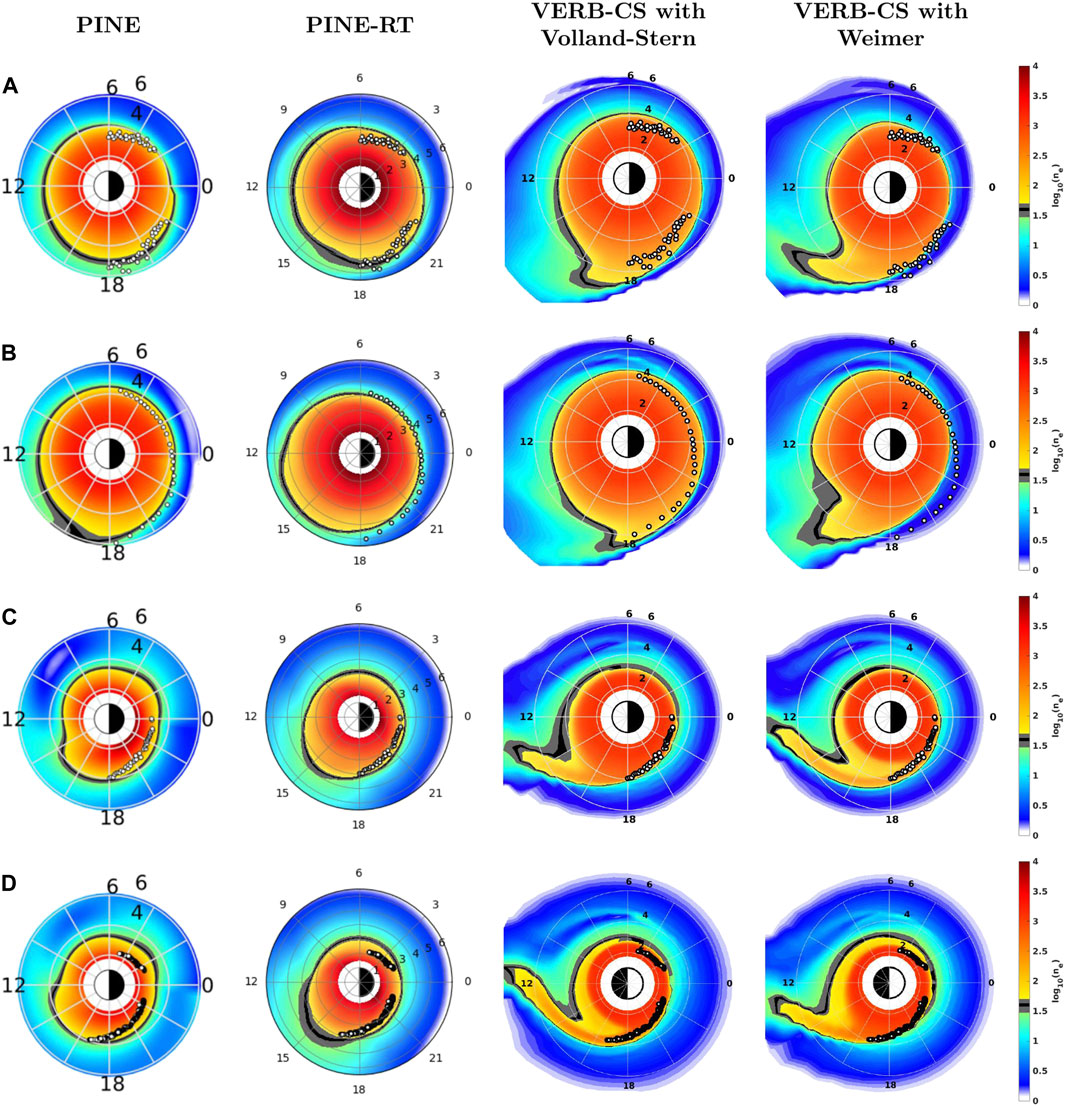
FIGURE 10. Comparison of the outputs of the PINE-RT model, of the PINE model and of the physics-based model driven by the Vollad-Stern and by the Weimer electric field models for events characterized by different levels of geomagnetic activity and occurred in the period March 2001 - June 2001. The color indicates the log10 of the plasma density (the scale of the colorbar is the same for all models and all times). The black-and-white dots show the location of the plasmapause derived from the IMAGE EUV images. The gray and black section of the colorbar indicates the density threshold of 40 ± 10 el/cm³, which is considered as an approximation of the plasmapause location. The Sun is to the left. Event (A): 11 Apr 2001 00:14 UT, Kp = 3. Event (B): 18 June 2001 03:45 UT, Kp = 4+. Event (C): 09 May 2001 18:13 UT, Kp = 5. Event (D): 20 March 2001 09:33 UT, Kp = 5.7.

It is also of interest the Event (b), for which the Weimer electric field model leads to an underestimation of the density in line of what was found on the Van Allen Probes data in Subsection 3.1. Despite the fact that the Weimer model promises a more detailed description of the electric field with its higher time resolution and its ability to show more complex field patterns, our simulations do not show that it also leads to more accurate results.

Finally we note that the VERB-CS model predicts plumes where we do not have the plasmapause data. The statistical evaluation of the performance of the models with regard to the prediction of the plumes is deferred to future studies and has not been the subject of this investigation.

4 Discussion

We reported here our efforts in developing a nowcast machine-learning model of the plasma density in the plasmasphere in the context of the PAGER project. We followed the approach of the PINE model (Zhelavskaya et al., 2017; Zhelavskaya et al., 2021) and we developed a feedforward neural network model of the plasma density in the equatorial plane. We explored several combinations of input features whose measurements and forecasts are available in the PAGER project, which are the Kp index and the solar wind properties at the L1 Lagrange point. We selected the best model, which is a neural-network model which takes the Kp index, vB_s, ρ_p and their last-three-days time history as input. The resulting model, which we call PINE-RT, is quite simple since it is composed of just one hidden layer with 15 neurons.

We validated the PINE-RT machine-learning model and compared it to the VERB-CS and PINE models of (Zhelavskaya et al., 2021). For this scope we performed a long-term study using in situ plasma density inferred from the plasma-wave measurements of the Van Allen Probes. Moreover, we evaluated the global plasmaspheric reconstructions against the plasmapause locations extracted from IMAGE EUV images on selected events. The PINE-RT model shows a performance comparable to the ones of the PINE model and of the VERB-CS model driven by the Volland-Stern electric field. In particular, it has a performance slightly worse than the one of the PINE model, which uses the geomagnetic indices AE, Kp, Sym-H, and F10.7 as inputs, and slightly better than the one of the VERB-CS model. The PAGER project is close to its end, but in a possible follow-up project we will explore the availability or the development of models predicting AE, Sym-H, and F10.7, such as Siciliano et al. (2021); Iong et al. (2022); Pallocchia et al. (2008); Pallocchia et al. (2021). In case of their availability, it will be interesting to compare the performances of the PINE-RT model with the one of the PINE model when driven by the respective predicted inputs. However, it should be noted that it remains to be seen if the latter model will be successful as the predicted AE, Sym-H, and F10.7 will have their own uncertainties. Moreover we believe that the PINE-RT model represents an important step towards having a plasmasphere model depending only on solar-wind features, which are the drivers of geomagnetic disturbances.

We considered quiet geomagnetic conditions and moderate storms (Kp < = 7). As future work, we want to broaden the applicability of the PINE-RT model to strong storms (Kp > 7) and perform a statistical study on plumes prediction. For this scope, data augmentation techniques will be needed in order to overcome the data scarcity. An interesting technique in this respective is the rebalancing, which was successfully applied for the Kp prediction in (Shprits et al., 2019). Another interesting idea is to add simulation results of the physics-based model to the training dataset of the machine-learning model, since (Zhelavskaya et al., 2021) showed that the physics-based model is able to describe some events with Kp > = 8. By doing this, we also expect to improve the capability of the PINE-RT model in reproducing the plume structures, since the physics-based model predicts the plume structures in all storms of our knownledge as a consequence of the convection mechanism.

We deployed the machine-learning model on the PAGER servers and it currently runs every hour predicting the next-day forecast of the plasma density in the equatorial plane. It combines the sources of the Kp index and of the solar wind features which are available in the PAGER project, using both the measurements and the forecasts available. The forecast of the model is available as a movie, which is updated every hour on the PAGER website18 and the nowcast is also available in near-real time throught the iSWA service of the Community Coordinated Modeling Center.

Even if beyond the needs of the PAGER project, it is of interest to consider whether our model of the plasma density in the equatorial plane can be extended to the whole plasmasphere. One way would be to use the model of Denton et al., 2002; Denton et al., 2004) or any other empirical model to extrapolate the density along the geomagnetic field lines. One can also train a full 3D model (e.g., Chu X. N. et al. (2017) and include in the training data observations far from the equatorial plane. However, such model will have much less training data and will have more degrees of freedom. The careful validation of such model would be critical to identify if there is sufficient data to derive the latitudinal distribution. Alternatively, one can train an empirical model of the latitudinal distribution that would depend on MLT and other input parameters. Such approach would still require a lot of data from different latitudes and the satellites would need to be carefully inter calibrated.

Data availability statement

The raw data supporting the conclusions of this article will be made available by the authors, without undue reservation.

Author contributions

SB developed the machine-learning model and implemented it for real-time runs. BH performed the simulations with the VERB-CS model. SB and BH prepared the manuscript. YS has conceived the study, supervised the project and helped in the preparation of the manuscript. YS is the PI of the PAGER project.

Funding

This project has received funding from the European Union’s Horizon 2020 research and innovation programme under grant agreement No. 870452 (PAGER).

Acknowledgments

We would like to acknowledge Ruggero Vasile and Irina Zhelavskaya for useful discussions during the development of the machine-learning model. Kp index and the plasma density inferred with the NURD algorithm are provided by GFZ, the solar wind data and the geomagnetic indices AE, F.10.7 and SYM-H by OMNIWebWe would like to thank the reviewers who contributed to improve this manuscript with their helpful suggestions.

Conflict of interest

The authors declare that the research was conducted in the absence of any commercial or financial relationships that could be construed as a potential conflict of interest.

Publisher’s note

All claims expressed in this article are solely those of the authors and do not necessarily represent those of their affiliated organizations, or those of the publisher, the editors and the reviewers. Any product that may be evaluated in this article, or claim that may be made by its manufacturer, is not guaranteed or endorsed by the publisher.

Footnotes

¹https://www.spacepager.eu/.

²https://iswa.gsfc.nasa.gov/IswaSystemWebApp/.

³https://omniweb.gsfc.nasa.gov/hw.html.

⁴https://scikit-learn.org/stable/modules/generated/sklearn.preprocessing.MinMaxScaler.html.

⁵https://scikit-learn.org/stable/modules/generated/sklearn.preprocessing.StandardScaler.html.

⁶https://scikit-learn.org/stable/modules/generated/sklearn.neural_network.MLPRegressor.html.

⁷https://www.swpc.noaa.gov/products/ace-real-time-solar-wind.

⁸https://www.spacepager.eu/work-packages/wp2.

⁹https://www.swpc.noaa.gov/products/3-day-geomagnetic-forecast.

¹⁰https://www.spacepager.eu/data-products/forecast-of-the-kp-index.

¹¹https://www.spacepager.eu/data-products/forecast-of-plasma-density.

¹²https://iswa.gsfc.nasa.gov/IswaSystemWebApp/.

¹³https://www.docker.com/resources/what-container.

¹⁴https://kubernetes.io/.

¹⁵https://omniweb.gsfc.nasa.gov/hw.html.

¹⁶https://image.gsfc.nasa.gov/.

¹⁷https://enarc.space.swri.edu/EUV/.

¹⁸https://www.spacepager.eu/data-products/forecast-of-plasma-density.

References

Aseev, N. A., and Shprits, Y. Y. (2019). Reanalysis of ring current electron phase space densities using van allen probe observations, convection model, and log-normal kalman filter. Space weather. 17, 619–638. doi:10.1029/2018SW002110

CrossRef Full Text | Google Scholar

Bailey, G. J., Balan, N., and Su, Y. Z. (1997). The sheffield University plasmasphere ionosphere model - a review. J. Atmos. Solar-Terrestrial Phys. 59, 1541–1552. doi:10.1016/S1364-6826(96)00155-1

CrossRef Full Text | Google Scholar

Bortnik, J., Li, W., Thorne, R. M., and Angelopoulos, V. (2016). A unified approach to inner magnetospheric state prediction. J. Geophys. Res. Space Phys. 121, 2423–2430. doi:10.1002/2015JA021733

CrossRef Full Text | Google Scholar

Carpenter, D. L., and Anderson, R. R. (1992). An isee/whistler model of equatorial electron density in the magnetosphere. J. Geophys. Res. Space Phys. 97, 1097–1108. doi:10.1029/91JA01548

CrossRef Full Text | Google Scholar

Chen, A. J., Grebowsky, J. M., and Taylor, H. A. J. (1975). Dynamics of mid-latitude light ion trough and plasma tails. J. Geophys. Res. 80, 968–976. doi:10.1029/ja080i007p00968

CrossRef Full Text | Google Scholar

Chu, X., Bortnik, J., Li, W., Ma, Q., Denton, R., Yue, C., et al. (2017a). A neural network model of three-dimensional dynamic electron density in the inner magnetosphere. J. Geophys. Res. Space Phys. 122, 9183–9197. doi:10.1002/2017JA024464

CrossRef Full Text | Google Scholar

Chu, X. N., Bortnik, J., Li, W., Ma, Q., Angelopoulos, V., and Thorne, R. M. (2017b). Erosion and refilling of the plasmasphere during a geomagnetic storm modeled by a neural network. J. Geophys. Res. Space Phys. 122, 7118–7129. doi:10.1002/2017JA023948

CrossRef Full Text | Google Scholar

Craig, E. R., Steven, M. G., and Steven, G. T. (1993). A two-dimensional model of the plasmasphere: Refilling time constants. Planet. Space Sci. 41, 35–43. doi:10.1016/0032-0633(93)90015-t

CrossRef Full Text | Google Scholar

Denton, R. E., Goldstein, J., and Menietti, J. D. (2002). Field line dependence of magnetospheric electron density. Geophys. Res. Lett. 29, 58-1–58-4. doi:10.1029/2002GL015963

CrossRef Full Text | Google Scholar

Denton, R. E., Menietti, J. D., Goldstein, J., Young, S. L., and Anderson, R. R. (2004). Electron density in the magnetosphere. J. Geophys. Res. Space Phys. 109, A09215. doi:10.1029/2003JA010245

CrossRef Full Text | Google Scholar

Goldstein, J., Burch, J. L., and Sandel, B. R. (2005). Magnetospheric model of subauroral polarization stream. J. Geophys. Res. Space Phys. 110, 1–10. doi:10.1029/2005JA011135

CrossRef Full Text | Google Scholar

Goldstein, J., Sandel, B. R., Hairston, M. R., and Reiff, P. H. (2003a). Control of plasmaspheric dynamics by both convection and sub-auroral polarization stream. Geophys. Res. Lett. 30. doi:10.1029/2003GL018390

CrossRef Full Text | Google Scholar

Goldstein, J., Spasojević, M., Reiff, P. H., Sandel, B. R., Forrester, W. T., Gallagher, D. L., et al. (2003b). Identifying the plasmapause in image euv data using image rpi in situ steep density gradients. J. Geophys. Res. Space Phys. 108, 1147. doi:10.1029/2002JA009475

CrossRef Full Text | Google Scholar

Haas, B., Shprits, Y. Y., Allison, H. J., Wutzig, M., and Wang, D. (2023). A missing dusk-side loss process in the terrestrial electron ring current. Sci. Rep. 13, 970. doi:10.1038/s41598-023-28093-2

PubMed Abstract | CrossRef Full Text | Google Scholar

Hassoun, M. H. (1995). Fundamentals of artificial neural networks. Cambridge, MA: MIT Press.

Google Scholar

Haykin, S. (1994). Neural networks: A comprehensive foundation. New York: Macmillan.

Google Scholar

He, F., Zhang, X.-X., Lin, R.-L., Fok, M.-C., Katus, R. M., Liemohn, M. W., et al. (2017). A new solar wind-driven global dynamic plasmapause model: 2. Model and validation. J. Geophys. Res. Space Phys. 122, 7172–7187. doi:10.1002/2017JA023913

CrossRef Full Text | Google Scholar

Horne, R., Thorne, R., Shprits, Y., Meredith, N. P., Glauert, S. A., Smith, A. J., et al. (2005). Wave acceleration of electrons in the van allen radiation belts. Nature 437, 227–230. doi:10.1038/nature03939

PubMed Abstract | CrossRef Full Text | Google Scholar

Huba, J. D., Sazykin, S., and Coster, A. (2017). Sami3-rcm simulation of the 17 march 2015 geomagnetic storm. J. Geophys. Res. Space Phys. 122, 1246–1257. doi:10.1002/2016JA023341

CrossRef Full Text | Google Scholar

Huba, J., and Krall, J. (2013). Modeling the plasmasphere with Sami3. Geophys. Res. Lett. 40, 6–10. doi:10.1029/2012GL054300

CrossRef Full Text | Google Scholar

Iong, D., Chen, Y., Toth, G., Zou, S., Pulkkinen, T., Ren, J., et al. (2022). New findings from explainable sym-h forecasting using gradient boosting machines. Space weather. 20, e2021SW002928. doi:10.1029/2021SW002928

CrossRef Full Text | Google Scholar

Kletzing, C., Kurth, W., Acuna, M., MacDowall, R. J., Torbert, R. B., Averkamp, T., et al. (2013). The electric and magnetic field instrument suite and integrated science (EMFISIS) on RBSP. Space Sci. Rev. 179, 127–181. doi:10.1007/s11214-013-9993-6

CrossRef Full Text | Google Scholar

Krall, J., and Huba, J. D. (2013). Sami3 simulation of plasmasphere refilling. Geophys. Res. Lett. 40, 2484–2488. doi:10.1002/grl.50458

CrossRef Full Text | Google Scholar

Li, W., and Hudson, M. (2019). Earth’s van allen radiation belts: From discovery to the van allen probes era. J. Geophys. Res. Space Phys. 124, 8319–8351. doi:10.1029/2018JA025940

CrossRef Full Text | Google Scholar

Matzka, J., Stolle, S., Yamazaki, Y., Bronkalla, O., and Morschhauser, A. (2021). The geomagnetic Kp index and derived indices of geomagnetic activity Space Weather. doi:10.1029/2020sw002641

CrossRef Full Text | Google Scholar

Mauk, B., Fox, N. J., Kanekal, S. G., Kessel, R. L., Sibeck, D. G., and Ukhorskiy, A. (2013). Science objectives and rationale for the radiation belt storm probes mission. Space Sci. Rev. 179, 3–27. doi:10.1007/s11214-012-9908-y

CrossRef Full Text | Google Scholar

Maynard, N. C., and Chen, A. J. (1975). Isolated cold plasma regions: Observations and their relation to possible production mechanisms. J. Geophys. Res. 80, 1009–1013. doi:10.1029/JA080I007P01009

CrossRef Full Text | Google Scholar

Mazzella, J., and Andrew, J. (2009). Plasmasphere effects for gps tec measurements in North America. Radio Sci. 44. doi:10.1029/2009RS004186

CrossRef Full Text | Google Scholar

Orlova, K., Shprits, Y., and Spasojevic, M. (2016). New global loss model of energetic and relativistic electrons based on van allen probes measurements. J. Geophys. Res. Space Phys. 121, 1308–1314. doi:10.1002/2015JA021878

CrossRef Full Text | Google Scholar

Pallocchia, G., Amata, E., Consolini, G., Marcucci, M., and Bertello, I. (2008). Ae index forecast at different time scales through an ann algorithm based on l1 imf and plasma measurements. J. Atmos. Solar-Terrestrial Phys. 70, 663–668. doi:10.1016/j.jastp.2007.08.038

CrossRef Full Text | Google Scholar

Pallocchia, G., Amata, E., Consolini, G., Marcucci, M., Bertello, I., and Flohrer, T. (2021). Medium-term predictions of f10.7 and f30 cm solar radio flux with the adaptive kalman filter. Astrophysical J. Suppl. Ser. 254, 9. doi:10.3847/1538-4365/abef6d

CrossRef Full Text | Google Scholar

Pierrard, V., Goldstein, J., André, N., Jordanova, V. K., Kotova, G. A., Lemaire, J. F., et al. (2009). Recent progress in physics-based models of the plasmasphere. Space Sci. Rev. 145, 193–229. doi:10.1007/s11214-008-9480-7

CrossRef Full Text | Google Scholar

Pierrard, V., Khazanov, G. V., Cabrera, J., and Lemaire, J. (2008). Influence of the convection electric field models on predicted plasmapause positions during magnetic storms. J. Geophys. Res. Space Phys. 113. doi:10.1029/2007JA012612

CrossRef Full Text | Google Scholar

Pierrard, V., and Stegen, K. (2008). A three-dimensional dynamic kinetic model of the plasmasphere. J. Geophys. Res. Space Phys. 113. doi:10.1029/2008JA013060

CrossRef Full Text | Google Scholar

Reeves, G. D., Spence, H. E., Henderson, M. G., Morley, S. K., Friedel, R. H. W., Funsten, H. O., et al. (2013). Electron acceleration in the heart of the van allen radiation belts. Science 341, 991–994. doi:10.1126/science.1237743

PubMed Abstract | CrossRef Full Text | Google Scholar

Ridley, A., Dodger, A. M., and Liemohn, M. W. (2014). Exploring the efficacy of different electric field models in driving a model of the plasmasphere. J. Geophys. Res. Space Phys. 119, 4621–4638. doi:10.1002/2014JA019836

CrossRef Full Text | Google Scholar

Sandel, B., Broadfoot, A., Curtis, C. C., King, R. A., Stone, T. C., Hill, R. H., et al. (2000). Identifying the plasmapause in image euv data using image rpi in situ steep density gradients. Space Sci. Rev. 91, 1147–1242. doi:10.1029/2002JA009475

CrossRef Full Text | Google Scholar

Schulz, M., and Lanzerotti, L. J. (1974). “Particle diffusion in the radiation belts,” in Physics and chemistry in space (Berlin, Heidelberg: Springer). doi:10.1007/978-3-642-65675-0

CrossRef Full Text | Google Scholar

Sheeley, B., Moldwin, M., Rassoul, H., and Anderson, R. (2001). An empirical plasmasphere and trough density model: Crres observations. J. Geophys. Res. 106, 25631–25641. doi:10.1029/2000JA000286

CrossRef Full Text | Google Scholar

Shprits, Y. Y., Kellerman, A. C., Drozdov, A. Y., Spence, H. E., Reeves, G. D., and Baker, D. N. (2015). Combined convective and diffusive simulations: VERB-4D comparison with 17 march 2013 van allen probes observations. Geophys. Res. Lett. 42, 9600–9608. doi:10.1002/2015GL065230

CrossRef Full Text | Google Scholar

Shprits, Y., Drozdov, A., Spasojevic, M., Kellerman, A. C., Usanova, M. E., Engebretson, M. J., et al. (2016). Wave-induced loss of ultra-relativistic electrons in the van allen radiation belts. Nat. Commun. 7, 12883. doi:10.1038/ncomms12883

PubMed Abstract | CrossRef Full Text | Google Scholar

Shprits, Y. Y., Allison, H. J., Wang, D., Drozdov, A., Szabo-Roberts, M., Zhelavskaya, I., et al. (2022). A new population of ultra-relativistic electrons in the outer radiation zone. J. Geophys. Res. Space Phys. 127, e2021JA030214. doi:10.1029/2021JA030214

CrossRef Full Text | Google Scholar

Shprits, Y. Y., Subbotin, D. A., Meredith, N. P., and Elkington, S. R. (2008). Review of modeling of losses and sources of relativistic electrons in the outer radiation belt ii: Local acceleration and loss. J. Atmos. Solar-Terrestrial Phys. 70, 1694–1713. doi:10.1016/j.jastp.2008.06.014

CrossRef Full Text | Google Scholar

Shprits, Y. Y., Vasile, R., and Zhelavskaya, I. S. (2019). Nowcasting and predicting the kp index using historical values and real-time observations. Space weather. 17, 1219–1229. doi:10.1029/2018SW002141

CrossRef Full Text | Google Scholar

Siciliano, F., Consolini, G., Tozzi, R., Gentili, M., Giannattasio, F., and De Michelis, P. (2021). Forecasting sym-h index: A comparison between long short-term memory and convolutional neural networks. Space weather. 19, e2020SW002589. doi:10.1029/2020SW002589

CrossRef Full Text | Google Scholar

Spasojević, M., Goldstein, J., Carpenter, D. L., Inan, U. S., Sandel, B. R., Moldwin, M. B., et al. (2003). Global response of the plasmasphere to a geomagnetic disturbance. J. Geophys. Res. Space Phys. 108, 1340. doi:10.1029/2003JA009987

CrossRef Full Text | Google Scholar

Stern, D. P. (1975). The motion of a proton in the equatorial magnetosphere. J. Geophys. Res. 80, 595–599. doi:10.1029/JA080I004P00595

CrossRef Full Text | Google Scholar

Stern, D. P. (1983). The origins of birkeland currents. Rev. Geophys. Space Phys. 21, 125–138. doi:10.1029/rg021i001p00125

CrossRef Full Text | Google Scholar

Subbotin, D. A., Shprits, Y. Y., and Ni, B. (2011). Long-term radiation belt simulation with the verb 3-d code: Comparison with crres observations. J. Geophys. Res. Space Phys. 116. doi:10.1029/2011JA017019

CrossRef Full Text | Google Scholar

Subbotin, D. A., and Shprits, Y. Y. (2009). Three-dimensional modeling of the radiation belts using the versatile electron radiation belt (verb) code. Space weather. 7. doi:10.1029/2008SW000452

CrossRef Full Text | Google Scholar

Tsyganenko, N. A. (1989). A magnetospheric magnetic field model with a warped tail current sheet. Planet. Space Sci. 37, 5–20. doi:10.1016/0032-0633(89)90066-4

CrossRef Full Text | Google Scholar

Volland, H. (1973). A semiempirical model of large-scale magnetospheric electric fields. J. Geophys. Res. 78, 171–180. doi:10.1029/JA078I001P00171

CrossRef Full Text | Google Scholar

Weimer, D. R. (2005). Improved ionospheric electrodynamic models and application to calculating Joule heating rates. J. Geophys. Res. Space Phys. 110, A05306–A05321. doi:10.1029/2004JA010884

CrossRef Full Text | Google Scholar

Xiong, C., Stolle, C., and Lühr, H. (2016). The swarm satellite loss of gps signal and its relation to ionospheric plasma irregularities. Space weather. 14, 563–577. doi:10.1002/2016SW001439

CrossRef Full Text | Google Scholar

Zhelavskaya, I. S., Aseev, N. A., and Shprits, Y. Y. (2021). A combined neural network- and physics-based approach for modeling plasmasphere dynamics. J. Geophys. Res. Space Phys. 126. doi:10.1029/2020JA028077

CrossRef Full Text | Google Scholar

Zhelavskaya, I., Shprits, Y., Spasojevic, M., and Kurth, W. (2020). Electron density derived with the neural-network-based upper-hybrid resonance determination algorithm from the van allen probes emfisis measurements. GFZ Data Serv. 2020. doi:10.5880/GFZ.2.8.2020.002

CrossRef Full Text | Google Scholar

Zhelavskaya, I. S., Shprits, Y., and Spasojević, M. (2017). Empirical modeling of the plasmasphere dynamics using neural networks. J. Geophys. Res. Space Phys. 122, 11,227–11,244. doi:10.1002/2017JA024406

CrossRef Full Text | Google Scholar

Zhelavskaya, I. S., Spasojevic, M., Shprits, Y. Y., and Kurth, W. S. (2016). Automated determination of electron density from electric field measurements on the van allen probes spacecraft. J. Geophys. Res. Space Phys. 121, 4611–4625. doi:10.1002/2015JA022132

CrossRef Full Text | Google Scholar