Creating a new paradigm for the local interstellar medium–A perspective

1 Introduction

As high-resolution spectra of narrow interstellar absorption lines in the sight lines to nearby stars became available, first in the optical (lines of Ca II and Ti II) and later in the ultraviolet, it became clear that parcels of interstellar gas distributed across a wide range of Galactic coordinates share common velocity vectors. For example, Crutcher. (1982) found that in the anti-Galactic center direction the gas has radial velocities consistent with a single velocity vector. This vector is now called the Local Interstellar Cloud (LIC), because neutral helium flowing into the heliosphere from the LISM has a velocity roughly consistent with this vector. Similarly, Lallement and Bertin. (1992) identified a different velocity vector for sight lines in the Galactic center direction that they called the Galactic cloud, which is now called the G cloud. The two high-resolution ultraviolet spectrographs on the Hubble Space Telescope, the Goddard High-Resolution Spectrograph (GHRS) and the Space Telescope Imaging Spectrograph (STIS), now provide the lion’s share of data on the LISM, because at the very low densities in the LISM almost all ions and atoms are populated only in their lowest energy states and transitions to the next higher energy states are mostly in the ultraviolet.

2 The multi-cloud model: Assumptions and results

In Figure 1, STIS spectra of the star HD 9826 (Edelman et al., 2019) show narrow interstellar absorption lines of Mg II (279.2, 280.3 nm), Fe II (260.0 nm), and the D I Lyman-α (120.6 nm). These are the most useful diagnostic lines, because they are strong but not optically thick and because the range in atomic mass (between 2 and 26) permits a clean separation of thermal broadening from turbulent broadening using the equation for line width b² = 2kT/m + ξ², where T is the temperature and ξ is the turbulent velocity. As shown in this figure, the interstellar absorption along this sight line has three velocity components that can be resolved in the Mg II and Fe II lines, but the separation of these components is not feasible for the low mass D I line because thermal broadening dominates. The central velocities of the three velocity components used in fitting the D I line are assumed to be the same as for the Mg II and Fe II lines. The spectral resolutions of the HST/STIS E230H mode used for observing the Mg II and Fe II lines and the E140H mode used for observing the D I line are about 3 km s⁻¹. If only lower spectral resolution data were available, the three velocity components could not be identified, in which case the line profile fitting procedure would have identified only a single very broad interstellar absorption line. We do not know what higher resolution spectra would show. Perhaps there are additional very narrow velocity components in this sight line indicative of very low temperature gas. There is at present no higher resolution UV spectrograph available or planned that could answer this question.

FIGURE 1

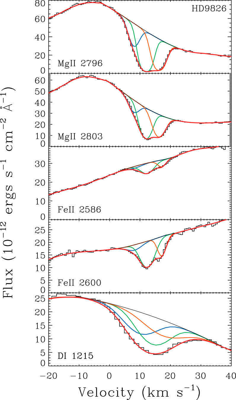
FIGURE 1. An example of a three velocity component fit to the star HD 9826 (F9 V). The separation of the three components is clearer in the high mass Fe II and Mg II spectral lines where thermal broadening is unimportant, but the three components are hard to distinguish in the D I Lyman-α line for which thermal broadening dominates. Figure from Edelman et al. (2019).

As described by Redfield and Linsky (2004a,b), the analysis of spectral data such as shown in Figure 1 proceeds through several steps. First, the stellar emission line is fit with a polynomial to provide the background emission line profile against which the interstellar absorption can be measured. Second, the interstellar absorption lines of Mg II and Fe II are fit with however many velocity components optimally fit the data. Since there are two Mg II lines and two useful Fe II lines, the interstellar parameters are fit for both lines simultaneously. With the obtained number of velocity components and their central velocities, we fit the D I interstellar absorption including both hyperfine transitions. The analysis of one spectral line in one sightline only provides information on the number of velocity components, their velocities and column densities. The combined analysis of several atoms or ions with very different masses leads to measured gas temperature, turbulent velocity, and other properties for each velocity component. The analysis of data from many sight lines leads to the identification of velocity vectors and thus clouds.

Using GHRS and STIS, Redfield and Linsky (2008) identified 15 clouds, each with its own velocity vector, located within about 15 pc of the Sun. The clouds are located closer than the distance to the nearest star with interstellar absorption consistent with this velocity vector. In their later analysis of interstellar spectra, Malamut et al. (2014) observed 34 new sight lines with 76 velocity components that are mostly consistent with the 15 previously identified clouds. More recently, Linsky et al. (2019) obtained a three dimensional model of the LIC using 62 sight lines covering about 45% of the sky. The model clearly shows that the Sun is located at the very edge of the LIC. The small difference between the mean speed and direction of the LIC flow compared to neutral helium flowing into the heliosphere (Swaczyna et al., 2021) indicates that the interstellar medium close to the heliosphere is not representative of the mean kinematics of the LIC. More about this in Section 3.5.

While the multi-cloud model proposed by Redfield and Linsky (2008) is robust in predicting radial velocities of interstellar gas in the new observations, the model is based on many assumptions that may not be realistic. They made these assumptions in order to simplify the analysis of a limited data set, but future analyses of larger data sets could lead to models with less restrictive assumptions. The assumptions of the multi-cloud model are.

• Definition of a cloud: A cloud is defined as a co-moving parcel of gas for which the measured radial velocities in sight lines toward stars covering a wide range of Galactic coordinates are consistent with a velocity vector to within the 2 km s⁻¹ absolute accuracy of STIS high-resolution spectra. The clouds contain partially ionized hydrogen and are warm, typically 3,000–12,000 K.

• Cloud locations, edges, and overlap: To simplify the analysis, the clouds are assumed to have definite edges and not overlap. Magnetic fields could explain the cloud edges, but the location of a cloud along a given sight line is uncertain. If there are several clouds along a sight line, the relative location of each cloud is unknown.

• Rigid motion: Each cloud is assumed to be a rigid co-moving structure containing gas that moves with the same velocity, but this assumption is unlikely to be realistic given the low densities and likely shocks or waves in the interstellar medium.

• Line broadening: The gas in a cloud is assumed to have a single temperature described by a Maxwellian velocity distribution and constant turbulent motions. Possible supra-thermal motions are not considered but could be important (Swaczyna et al., 2019).

• Contiguous structure: Each cloud is assumed to be contiguous without isolated structures.

• Cloud boundaries and homogeneous density: The linear dimensions of clouds are measured by their neutral hydrogen absorption. The length of a cloud along sight line is l = N (H I)/n (H I), where N (H I) is the neutral hydrogen column density and n (H I) is the neutral hydrogen number density. Since the hydrogen Lyman-α line is extremely optically thick at line center, τ(0) = 10⁵–10⁶, N (H I) is obtained from the deuterium Lyman-α line with N (H I) = N (D I)/(D/H), where (D/H) = 1.56 × 10^–5 is the deuterium to hydrogen number density in the LISM (Wood et al., 2004). However, there have been no estimates of n (H I) except for the LIC. In Section 3.3, we will describe a method for estimating n (H I) in other clouds.

• Inter-cloud gas? Hydrogen in the gas between and surrounding clouds must be fully ionized otherwise the inter-cloud gas would be detected as a cloud. The ionized hydrogen could be hot (10⁶ K) or warm (10⁴ K) gas photo-ionized by a nearby hot star or white dwarf.

With these assumptions, Redfield and Linsky. (2008) created a two dimension map for the cloud locations and sizes in Galactic coordinates. Vannier et al. (2022) traced the path of the Sun through nearby clouds from 150,000 years in the past to 60,000 years in the future. In this model the Sun entered the LIC about 60,000 years ago and will leave the LIC very soon to enter the G cloud.

3 Challenges to the multi-cloud model

Despite the successes of the multi-cloud model with rigid clouds, there have been a number of challenges to the underlying assumptions.

3.1 The Gry-Jenkins non-rigid single cloud model

Gry and Jenkins. (2014) challenged the multi-cloud model by proposing that the neutral hydrogen gas within 10 pc of the Sun lies within a single cloud that has a positive velocity gradient in the direction of its motion. With this model they were able to fit the observed radial velocities of most of the observed velocity components. A shock proceeding through the cloud fits most of the remaining velocity components. They argued that their model is simpler than the multi-cloud model and probably more realistic.

Redfield and Linsky. (2015) used the data presented in Malamut et al. (2014) to test the predictive abilities of the multi-cloud model and the Gry-Jenkins one-cloud model with a new HST data set. SNAP observations with HST are designed to fill one-orbit gaps between large observing programs with short programs selected from accepted target lists by the telescope schedulers in order to minimize telescope slewing time. Redfield and collaborators proposed a long list of LISM targets across the sky from which HST observed 32 targets. Essentially all of the velocity components in these new sight lines match the radial velocities of the previously identified clouds in their directions. A test of these two models was provided by the errors between the observed radial velocities in the SNAP data and the radial velocities predicted by each model. Redfield and Linsky. (2015) found the root-mean-square errors are much smaller for the multi-cloud model than for the Gry-Jenkins model, however the multi-cloud model has many more free parameters that should lead to a tighter fit to the radial velocity data. Thus it is not yet clear which model is a better representation of the LISM.

3.2 Non-homogeneous cloud properties

The number of sight lines observed by HST has now increased enough to support a more detailed statistical analysis of the LISM data. Linsky et al. (2022) analyzed the temperatures and turbulent velocities of 84 velocity components, 36 of which traverse the LIC. A wide distribution of temperatures extends from about 3,000 K to more than 12,000 K, even for the LIC only sight lines. The broad Gaussian fits to the data suggest that the range of temperatures is random with perhaps an overabundance of high temperature components. Turbulent velocities show a similar pattern with a large range between 0 and 5 km s⁻¹ for both the LIC only data and the entire LISM data set. The temperature differences of LIC plasma in pairs of sight lines far exceed the mean measurement errors. For the Procyon-AD Leo sight line pair, which has the smallest angular separation (2°.2), the temperature difference is 2, 200 ± 450 K. The three sight line pairs with the next larger angular separations show similar temperature differences that are 3-4 times the measurement errors. The angular separation of 2°.2 corresponds to a linear separation of 5,100 au near the center of the LIC. Since the Sun moves 5.1 au/year through the LIC, the heliosphere should see significant temperature differences in its interstellar environment on a time scale of less than 1,000 years.

Linsky et al. (2022) also searched for significant dependancies of temperatures and turbulent velocities with respect to different parameters. None were detected with respect to Galactic coordinates, angle relative to the neutral helium inflow direction, LISM magnetic field direction, EUV radiation field, or hydrogen column density. A test of whether temperatures and turbulent velocities through the LIC depend on angle relative to the LIC center also showed no significant dependence.

3.3 Neutral hydrogen density in clouds

For more than 15 years, the consensus has been that the neutral hydrogen density in the LIC is n (H I) ≈ 0.20 cm⁻³. This conclusion was based on the measurement of the neutral helium density in the gas flowing into the heliosphere and the He/H number density (see Swaczyna et al. (2020) and references therein). Also, theoretical models using the Cloudy photoionization code by Slavin and Frisch. (2008) resulted in n (H I) = 0.195 ± 0.05 cm⁻³. The analysis of 37 sight lines to stars within 10 pc of the Sun by Linsky and Redfield. (2021) provided a different answer; Figure 2 shows that for these velocity components the cloud filling factor is ff = d/n (H I), where d is the distance to the star and n (H I) = 0.20 cm⁻³. With only one exception, toward the star AD Leo (see Section 3.5), all filling factors are less than 0.63 and most are much smaller. For sight lines shorter than 4 pc, the mean filling factor is about 0.5, corresponding to n (H I) = 0.10 cm⁻³ filling the entire sight line, not 0.20 cm⁻³. Four of the stars with only a LIC component within 4 pc of the Sun have astrospheres evidenced by hydrogen wall absorption seen as red-shifted absorption in the Lyman-α line. These stars must, therefore, be in an interstellar environment containing neutral hydrogen extending from the heliosphere all of the way to the star. Therefore, n (H I) ≈ 0.10 cm⁻³ toward these four stars and likely the other sight lines within 4 pc. For the more distant stars, either the entire sight line is filled with lower density clouds, or, more likely, the more distant clouds also have densities with n (H I) ≈ 0.10 cm⁻³, and there is inter-cloud gas with fully ionized hydrogen between these clouds.

FIGURE 2

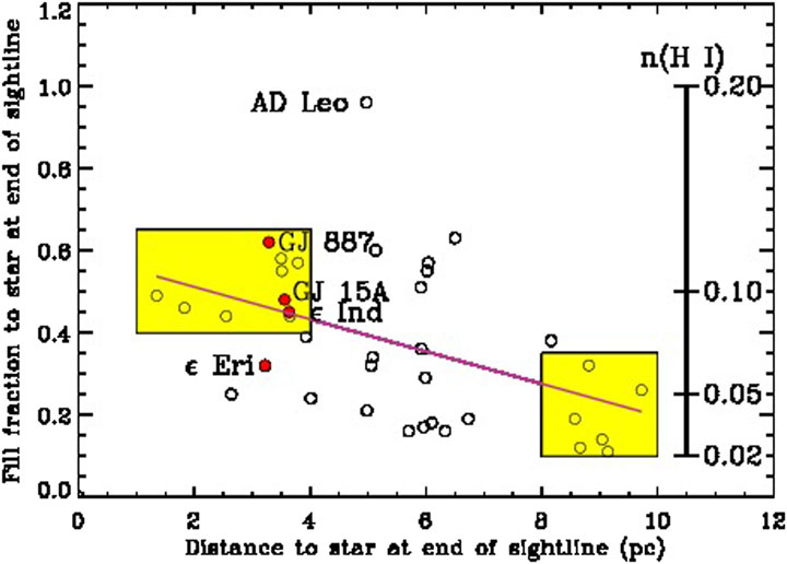
FIGURE 2. Plot of the filling fraction of neutral hydrogen clouds along sight lines to stars vs. stellar distance. On the right side is the scale of neutral hydrogen density if the sight lines are completely filled with clouds. The left colored box identifies sight lines that would be filled by clouds with a mean density n(H I)$\approx 0.10$ cm⁻³. The right colored box identifies sight lines with distant clouds that are widely separated. The 4 stars within 4 pc of the Sun with only LIC and astrospheric absorption are identified in the figure. Figure from Linsky and Redfield, 2021.

3.4 Are clouds isolated or tightly packed?

In the multi-cloud model, the cloud sizes were determined assuming n (H I) = 0.20 cm⁻³, leading to the clouds being separated by inter-cloud gas even within 4 pc. If instead, neutral hydrogen densities in the clouds are about 0.10 cm⁻³, then the clouds have linear dimensions twice as large and the LISM is completely filled with no space available for inter-cloud gas at least within 4 pc. Thus the clouds are tightly packed and could overlap.

3.5 Do clouds overlap or merge?

Recently, Swaczyna et al. (2022) proposed that very adjacent to the heliosphere there is a region of mixed LIC and G clouds with temperature, speed, and direction intermediate between the mean LIC and G cloud parameters. This mixed cloud model solves a number of problems. First, it explains why the properties of neutral helium flowing into the heliosphere has a slightly different temperature and velocity than the mean LIC parameters. Second, it explains why the inflowing interstellar gas has a density n (H I) = 0.20 cm⁻³. This density is the sum of the LIC and G clouds. Third, this model explains why ff = 1.0 and therefore n (H I) = 0.20 cm⁻³ toward AD Leo. It turns out that the sight line to AD Leo is where the mixed clouds have the longest path length. Since in the overlap region the properties of the gas is intermediate between the LIC and G clouds, this is a mixed cloud with intermediate properties.

4 Towards a possible new model for the LISM

LISM studies have evolved greatly from the kinematic identification of clouds with uniform properties to a more complex structure of inhomogeneous clouds that fill the local environment or one cloud with complex internal velocity structure. Within about 4 pc of the Sun, partially ionized clouds appear to completely fill space with no ionized inter-cloud medium. The overlap or mixing of adjacent clouds is likely common with the mixed LIC-G cloud as the prototype. Other mixed clouds should be searched for in the existing and future data. The physical processes that occur when clouds overlap and merge is only beginning to be understood presently based on only one example. Perhaps the multi-cloud model could be revised to include cloud overlap regions with intermediate velocities that may explain the velocity components that presently do not have assigned clouds. A fully three-dimensional model of the distribution of LISM clouds is needed in order to evaluate the filling factor and extent of cloud overlap, and to assess the near term evolution and consequences of such a new model for the LISM.

Facilities: HST (STIS), HST (HRS), Voyager I, Voyager II.

Data availability statement

Publicly available datasets were analyzed in this study. This data can be found here: https://iopscience.iop.org/article/10.3847/1538-3881/ac816b.

Author contributions

This paper provides a perspective on the local interstellar medium and how the present paradigm will likely change.

Acknowledgments

We gratefully acknowledge support from NASA Grant 80NSSC20K0785. JL thanks the conference “Ultraviolet Astronomy in the XXI Century” for the environment at which this paper was developed.

Conflict of interest

The authors declare that the research was conducted in the absence of any commercial or financial relationships that could be construed as a potential conflict of interest.

Publisher’s note

All claims expressed in this article are solely those of the authors and do not necessarily represent those of their affiliated organizations, or those of the publisher, the editors and the reviewers. Any product that may be evaluated in this article, or claim that may be made by its manufacturer, is not guaranteed or endorsed by the publisher.

References

Crutcher, R. M. (1982). The local interstellar medium. ApJ 254, 82. doi:10.1086/159707

CrossRef Full Text | Google Scholar

Edelman, E., Redfield, S., Linsky, J. L., Wood, B. E., and Müller, H. (2019). Properties of the interstellar medium along sight lines to nearby planet-hosting stars. ApJ 880, 117. doi:10.3847/1538-4357/ab1f6d

CrossRef Full Text | Google Scholar

Gry, G., and Jenkins, E. B. (2014). The interstellar cloud surrounding the Sun: A new perspective. A&A 567, A58. doi:10.1051/0004-6361/201323342

CrossRef Full Text | Google Scholar

Lallement, R., and Bertin, P. (1992). Interstellar gas in the heliosphere and the solar wind anisotropies. Astron. Astrophys. 266, 479.

Google Scholar

Linsky, J. L., and Redfield, S. (2021). Could the local cavity be an irregularly shaped strömgren sphere?*. ApJ 920, 75. doi:10.3847/1538-4357/ac1feb

CrossRef Full Text | Google Scholar

Linsky, J. L., Redfield, S., Ryder, D., and Chasan-Taber, A. (2022). Inhomogeneity within local interstellar clouds*. Aj 164, 106. doi:10.3847/1538-3881/ac816b

CrossRef Full Text | Google Scholar

Linsky, J. L., Redfield, S., and Tilipman, D. (2019). The interface between the outer heliosphere and the inner local ISM: Morphology of the local interstellar cloud, its hydrogen hole, strömgren shells, and 60Fe accretion*. ApJ 886, 41. doi:10.3847/1538-4357/ab498a

CrossRef Full Text | Google Scholar

Malamut, C., Redfield, S., Linsky, J. L., Wood, B. E., and Ayres, T. R. (2014). THE STRUCTURE OF THE LOCAL INTERSTELLAR MEDIUM. VI. NEW Mg II, Fe II, AND Mn II OBSERVATIONS TOWARD STARS WITHIN 100 pc. ApJ 787, 75. doi:10.1088/0004-637x/787/1/75

CrossRef Full Text | Google Scholar

Redfield, S., and Linsky, J. L. (2004a). Astrophys. J. 602, 776.

Redfield, S., and Linsky, J. L. (2015). Evaluating the morphology of the local interstellar medium: Using new data to distinguish between multiple discrete clouds and a continuous medium. ApJ 812, 125. doi:10.1088/0004-637x/812/2/125

CrossRef Full Text | Google Scholar

Redfield, S., and Linsky, J. L. (2004b). The structure of the local interstellar medium. III. Temperature and turbulence. ApJ 613, 1004–1022. doi:10.1086/423311

CrossRef Full Text | Google Scholar

Redfield, S., and Linsky, J. L. (2008). The structure of the local interstellar medium. IV. Dynamics, morphology, physical properties, and implications of cloud-cloud interactions. ApJ 673, 283–314. doi:10.1086/524002

CrossRef Full Text | Google Scholar

Slavin, J. D., and Frisch, P. C. (2008). The boundary conditions of the heliosphere: Photoionization models constrained by interstellar and in situ data. A&A 491, 53–68. doi:10.1051/0004-6361:20078101

CrossRef Full Text | Google Scholar

Swaczyna, P., McComas, D. J., and Schwadron, N. A. (2019). Non-equilibrium distributions of interstellar neutrals and the temperature of the local interstellar medium. ApJ 871, 254. doi:10.3847/1538-4357/aafa78

CrossRef Full Text | Google Scholar

Swaczyna, P., McComas, D. J., Zirnstein, E. J., Sokół, J. M., Elliott, H. A., Bzowski, M., et al. (2020). Density of neutral hydrogen in the sun's interstellar neighborhood. ApJ 903, 48. doi:10.3847/1538-4357/abb80a

CrossRef Full Text | Google Scholar

Swaczyna, P., Rahmanifard, F., Zirnstein, E. J., McComas, D. J., and Heerikhuisen, J. (2021). Slowdown and heating of interstellar neutral helium by elastic collisions beyond the Heliopause. ApJL 911, L36. doi:10.3847/2041-8213/abf436

CrossRef Full Text | Google Scholar

Swaczyna, P., Schwadron, N. A., and Möbius, E. (2022). Mixing interstellar clouds surrounding the Sun. Astrophys. J. Lett. 937, 32. doi:10.3847/2041-8213/ac9120

CrossRef Full Text | Google Scholar

Vannier, H., Redfield, S., Wood, B. E., Múller, H. R., and Linsky, J. L. (2022). In prep.

Google Scholar