The pysat ecosystem

1 Introduction

The future expansion of scientific instrumentation will exacerbate the difficulties in finding, downloading, accessing, and utilizing space science data. Currently, data is stored and distributed by a variety of government, academic, and commercial agencies through a variety of mechanisms and file formats. While these specific mechanisms and formats may reflect the specific needs of a particular community it produces an additional challenge for scientists seeking to work with data across various sub-fields. Many problems require the integration and use of ground-based, space-based, and even modelled data to understand or answer science questions.

There are emerging solutions for cloud computing where the data and processing capabilities are hosted on remote servers that scientists can access. These services can be extremely useful, particularly within a community that has similar needs but differing funding levels. While this technique can make it easier for scientists to access and load data, the available data is limited to sets installed on the server. Thus, interdisciplinary users are likely to encounter situations where desired data sets may be distributed across multiple servers, similar to the current data distribution challenges. While users may be able to download data from different services on a computer they control, it is less likely that users will be able to upload their own data sets.

A shift to cloud computing also has negative implications for equitable and long term accessibility of data. Use of cloud computing has ongoing non-trivial costs and excels for situations where significant resources are needed for only a limited time. Users without funding, or additionally without access, like the public, would not be able to utilize those services for their own research. The ongoing costs for local hardware, by virtue of not including hardware costs as done in cloud computing, are lower. Further, administrative approval is not required for users to operate personal computers. Thus, software that supports scientific processing, including data downloads, on a user’s local machine (as well as via the cloud) provides the greatest accessibility and access for the largest number of people.

One approach for solving the data distribution and format issues is to mandate a single file format across a scientific discipline and create a super server, or single access point, for all data. The challenge with this type of solution is it ignores the historical reasons that created multiple file formats and access mechanisms in the first place. Typically speaking, each community within space science has its own requirements, based upon science focus, data type, and distribution mechanisms that evolved over time consistent with that particular communities needs. Mandating a single method or format across space science ignores these sub-field requirements. Working with a single general format everywhere is thus likely not possible, and at best sub-optimal, increasing the cost of working with data for everyone. A change in file format could also break existing systems. Further, unless all data in space science, as well as all disciplines that can impact space science, are all integrated into the same format and server, there will always be scientists that must work across formats and data sources.

While data discovery, download, and loading are significant challenges, scientific data also generally requires additional processing to be useful. Typically, at minimum, data must be selected for high quality observations (or cleaned). Depending upon the data set there may be flags included with the data. Alternately, the appropriate conditions for selecting from all available data may only be available in a scientific publication. Though there is a move towards greater access to publications the historical record is still typically confined behind a paywall. Even when readily accessible, the current situation requires researchers to construct code to properly clean data for robust scientific analysis.

The scientific community has been shifting from analyzing data from one or few platforms to working with multiple platforms, particularly for data assimilation or machine learning models. Working with multiple data sets involves additional challenges. While some analyses can work with multiple data sets individually, this is not always the case. When an individual data set approach is not possible, multiple data sets need to be loaded at once, where data from one source is used directly in the selection or processing of other data. Without a systematic framework to work with multiple data sources the practical challenges are likely to be solved sub-optimally, as pressures to produce results and publish can limit the quality, extensibility, and maintainability of the code produced.

The traditional instrument mission in space science required the concerted effort of multiple space scientists per instrument. This level of personnel is supportable when there are few spacecraft and the ground-based instrumentation is easily maintained. The rise of massive constellations with thousands of satellites, such as Starlink, cannot maintain the same staffing levels (Moigne, 2018). Further, one of the challenges when working with multiple instruments in a constellation is each instrument may have unique and unexpected characteristics that requires additional specialized processing. To enable science to make use of large constellations there is a need for software that can effectively scale the efforts of few scientists to many instruments, while accommodating the potentially unique processing requirements for individual instruments in the constellation.

The Python Satellite Data Analysis Toolkit (pysat) provides a community wide solution for these problems. The core pysat package provides a data-independent user interface that abstracts away the tedious details of file, data, and metadata handling so that scientists can focus on science. Pysat is designed as a data plug-in system where support for each data set includes functionality to download, load, process, and clean data. Plug-ins differ from modules in that plug-ins are not functional on their own and depend upon a host program to plug into. Further, users don’t generally interact with the plug-ins directly but through the host program, or pysat. This plug-in configuration supports any file format or data source. Further, it makes it possible for community members to distill their data knowledge into working code so that the community can automatically work with the best interpretation of data. In addition, the core pysat package includes a variety of standards and functionality tests so that developers of these plug-ins get direct feedback on standards compliance.

Support for a wide variety of data sets in pysat has been grouped by data provider and released as independent software packages. This configuration reduces the requirements for any given user as they only need to install the packages they need while offering the broadest array of instrument support in the open source community. The versatility and generality of these features makes it possible for pysat to support data from any provider and in any format. Rather than require all funding agencies to adopt the same standard, pysat is designed to interact with a variety of data sources and file formats but still provide a common and consistent interface for scientists. Thus, communities may maintain their specialized approaches as desired, while those that work across or within domains can do so through a consistent interface.

The array of pysat features are well suited for instrumentation processing. The data and metadata handling features reduces requirements on developers while maintaining the customizability needed for large constellations. Pysat is in use for Ion Velocity Meter (IVM) processing on both the NASA Ionospheric Connections (ICON) Explorer as well as the National Oceanic and Atmospheric Administration (NOAA)/National Space Organization (NSPO) Constellation Observing System for Meteorology Ionosphere and Climate-2 (COSMIC-2) constellation. Pysat features are also used to create the publicly distributed files for the missions.

Pysat is an open source package that builds upon the existing community of tools and is designed to interact with others (e.g., Burrell et al., 2018; Pembroke et al., 2022). In particular, pysat builds upon the pandas (pandas development team, 2022) and xarray (Hoyer et al., 2022) packages so that the general and scientific community use the same tools. This commonality reduces the barrier for the public to interact with scientific data, as well as making it more likely for pysat to expand beyond the currently supported community.

Pysat’s generalized features makes it well suited for any data set available from any source. The core pysat team are ionospheric scientists thus the data sets already supported by pysat reflect this scientific focus. However, pysat itself is not limited to ionospheric data, and pysat’s plug-in design makes it possible for users to add their own data to pysat. As such, pysat is suitable for use in industry, professional science, citizen science, and the classroom. To support this wider perspective pysat joined NumFOCUS as an affiliated package.

Since its original publication (Stoneback et al., 2018), pysat has broken out data support and analysis packages into an ecosystem. Features within pysat have also been expanded and generalized as needed. For clarity, this manuscript covers the advances within the core pysat package as part of a description of pysat’s larger feature set. Examples from each of the pysat ecosystem packages (collectively referred to as the pysat Penumbra) are also included. Analysis functionality has also been broken out into individual packages. This reconfiguration of pysat helps to minimize requirements on users and developers, while maintaining the same level of functionality. The ecosystem makes it easier for the wider community to contribute instrument support code as each pysat Penumbra package is focused and contains functions designed to work with a particular data source or perform a particular type of analysis. Pysat is a core package within the Python in Heliophysics Community (Burrell et al., 2018; Barnum et al., 2022) and is a community developed package.

2 Methods

2.1 Pysat

The main user interface is the pysat Instrument object. The Instrument object provides a consistent interface for working with data independent of source, abstracting away tedious file and data handling details. The Instrument object incorporates a data processing workflow to accommodate all of the versatility required for research data analysis within a systematic framework. Data can be loaded by users either by file or by specifying a time range in increments of days, independent of the time stored in a given file. The features in the Instrument object enables the construction of instrument independent analysis procedures that work independent of the data dimensions or source, and provides a foundation to transition to the analysis of many data sources with limited personnel.

A canonical example for working with any data set supported by pysat is included below.

First, relevant packages are imported and then a directory for pysat to store data is assigned. The pysat directory, or directories, only needs to be assigned once per installation. For this example we will work with the Solar Wind Electron Proton Alpha Monitor (SWEPAM) instrument on the Advanced Composition Explorer (ACE) spacecraft. Support for this data set is provided in the pysatSpaceWeather (Burrell et al., 2022b) package and must be registered once before use.

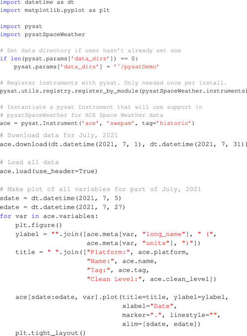
To accommodate the wide variety of data sources and file and metadata formats pysat is designed as a plug-in system. Support for a particular data set is enabled by an external module that implements a variety of methods required by pysat, including support for downloading, loading, and cleaning data. These modules ’plug-in’ to specific interfaces within pysat, are controlled by pysat, and aren’t functional on their own. As directed by a user, pysat will invoke these supporting functions as needed to provide data and metadata to pysat in appropriate formats. The configuration provides a consistent interface for the user while accommodating a wide variety of technical solutions for any particular data set.

A pysat instrument object for the ACE SWEPAM data is instantiated after the pysat directory is assigned. Data sets are labeled by up to four parameters: ‘platform’, ‘name’, ‘tag’, and ‘inst_id’. ‘Platform’ and ‘name’ are required and refer to the measurement platform and instrument name. ‘Tag’ and ‘inst_id’ may be used to further distinguish between multiple outputs from an instrument, or perhaps multiple data products from a given measurement platform (e.g., spacecraft, constellation, or observatory) and instrument combination.

Using the Instrument object the full life cycle for data analysis is enabled through class methods. Data is retrieved from the remote repository using the ‘ace.download’ command. The user specifies a range of dates and pysat calls the ACE SWEPAM support in pysatSpaceWeather to access the remote repository, retrieve the data, and store it locally. The files are organized under the pysat data directory assigned by the user. By default, data is organized under this user-specified directory using ‘platform’, ‘name’, ‘tag’, and ‘inst_id’ sub-directories, allowing simple machine and user file navigation.

All of the ACE SWEPAM data on a user’s system is loaded using the pysat Instrument class method ‘load’. A load command with no date restrictions will load all data on the user’s system. Note that no memory checks are performed before loading. This means that if a ‘.load()’ command is issued for a very large data set, pysat will attempt to load all of the data, even if it exceeds local memory. Alternately, a single date (specified by the year and day of year or a Python datetime object) or a range of dates may be provided.

To continue the canonical pysat code example, a range of dates is defined and each ACE SWEPAM variable is plotted as a function of time. Since files from different sources do not typically have the same metadata standards, pysat automatically translates loaded metadata into a set of labels that may be controlled by the user. Default metadata labels of ‘units’ and ‘name’ are used in this example. A selection of the plots produced from the code above are in Figure 1.

FIGURE 1

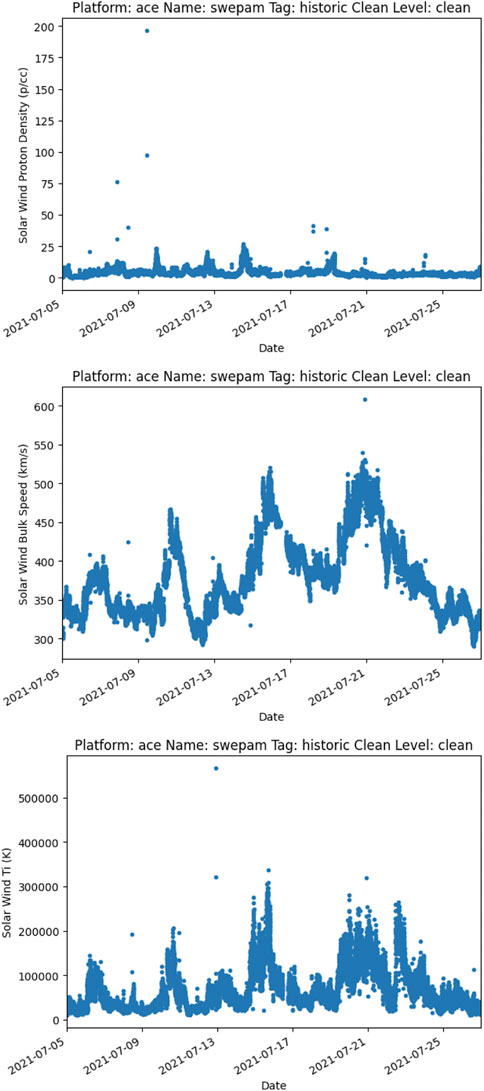
FIGURE 1. Selected output plots from ACE SWEPAM example.

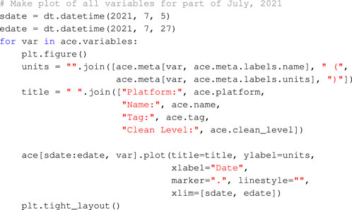
To support an even more generalized approach for cases where users assign non-default metadata labels developers may use the ‘meta.labels’ instance to access metadata as below. This ensures that regardless of the string values assigned to the Instrument object to identify ‘units’ or ‘name’ the code will continue to work. We emphasize the code below is not needed to account for different labels used within files as metadata labels are automatically translated to the standard assigned in the Instrument object.

The only portions of the canonical example code above that are specific to SWEPAM on ACE are the particular values of ‘platform’, ‘name’, and ‘tag’ when instantiating the Instrument. Updating those values for any of the other instruments within pysat will similarly download, load, and plot data in early July 2021, provided the data is available.

A listing of all data sets registered in pysat is available to the user with the ‘pysat.utils.display_available_instruments()’ function which prints the corresponding ‘platform’, ‘name’, ‘tag’, ‘inst_id’, and a short description for all registered plug-ins. Further, additional information may be obtained from each data plug-in module using the ‘help’ command. Similarly, help may be invoked on the ‘inst_module’ attribute attached to the pysat Instrument class for expanded information on the instantiated data set.

2.1.1 Data

Pysat also includes generalized data access at the Instrument level for ease of use and to support the construction of the generalized processing functions. Some instruments produce a collection of one dimensional signals that depend soley on time, while others require higher-dimensional structures. To support the widest variety of data sets pysat provides support for Instruments to utilize a pandas DataFrame or an xarray Dataset as the underlying data format. The DataFrame excels at tabular data, or a collection of one dimensional data in time. Higher dimensional data is better served using xarray, which builds upon pandas indexing to support higher dimensional data sets.

Similar to numpy (Harris et al., 2020), pandas, and xarray, the pysat Instrument supports a variety of indexing techniques for data access and assignment. These methods are shown below.

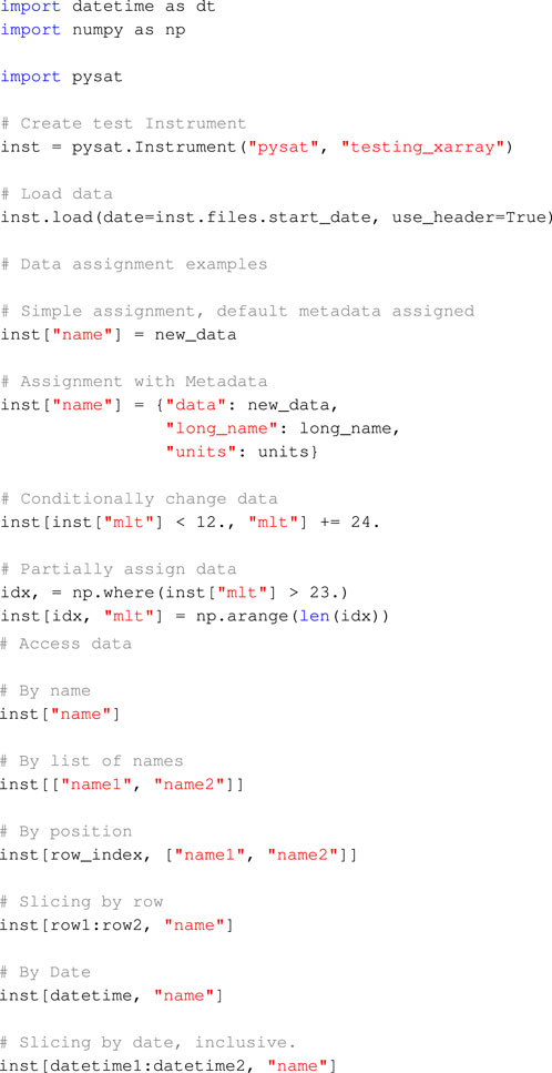
Though a simulated data set loaded into xarray is used here, the same commands also work for Instrument objects with pandas DataFrames as the underlying format. Variables can be selected singly or through a list of strings. Data may be down-selected using Boolean or integer indexing. Indexing functionality supports both one and higher dimensional data. While the access and assignment functionality should serve all developer needs the full data set is always available to users and developers at the ‘data’ Instrument attribute. Users and developers may access or modify the loaded data directly as needed.

The data access provided by pysat is primarily enabled by the underlying data formats. Pysat is simply mapping the inputs to the relevant underlying format. This simplifies the user’s experience, since these methods are not always treated identically by pandas and xarray. This general data support is a core functionality of pysat, and will be maintained if other internal data formats are introduced.

2.1.2 Metadata

Pysat also includes support for tracking metadata, so users can easily understand a data set they are working with and by accessing the data documentation provided in the original files. While xarray is equipped to track metadata for both individual variables and an entire data set, pandas is not equipped to do so. To ensure the most consistent user interface, pysat tracks metadata using its own class and is thus independent of the underlying data format.

Since file standards typically document metadata in different ways pysat builds in functionality to automatically translate metadata in the file to a user provided consistent standard. Pysat defaults to tracking seven different metadata parameters: Units, long name, notes, description, minimum, maximum, and fill value. The categories of metadata are used to automatically translate metadata as directly stored in a file to a standard set by the user. Users can track any number of desired parameters for individual variables. File-level metadata is stored using the file-specified attributes in the ‘meta.header’ class. This ensures all metadata provided within a file is accessible within the pysat Instrument without duplicating any data.

For ease of use, the metadata access is case preserving but case insensitive. Thus, using ‘units’ or ‘Units’ or any other variation in case returns or assigns the same data. This feature is intended to support broader compatibility of code written to a particular metadata standard.

Pysat’s metadata support is intended to support coupling metadata from any standard for use within pysat. As such, adopting a particular metadata file format for pysat compatibility is not strictly required. Maximum compatibility is achieved when the file metadata standard includes information in the seven categories that pysat tracks by default, as noted above. However, pysat supports additional categories as needed.

2.1.3 File handling and organization

Pysat’s Instrument class is intended to free users from specific knowledge about a data set’s files. Enabling this abstraction requires that pysat has knowledge about the files on the local system, obtained by parsing filenames. The file list is used by pysat when loading data, either through the ‘load’ class method, or through pysat’s built in iteration features. Information about local files is also used when updating a local data set for consistency with the most recent files at the data source.

Pysat requires that all of the data be placed in one or more user-specified high level directories. Nominally data sets are organized under the top-level directories using the corresponding values of ‘platform’, ‘name’, ‘tag’, and ‘inst_id’. Users can set their own preferred schema and utilities are included to move files from one schema to another. This preference may be assigned pysat wide using the parameters class, or an a per Instrument basis using the ‘directory_format’ Instrument keyword.

Pysat has file parsing utilities to properly categorize the date of the file, as well as parameters such as version, revision, or cycle. Users can direct pysat to parse out custom information as well. The informational structure of a filename is typically specified and used internally by a developer when constructing a pysat data set plug-in. Users can load data with a different filename structure, e.g., for files obtained from a non-default data provider, by setting the same information at Instrument instantiation with the ‘file_format’ keyword.

Pysat provides two functions for parsing filenames using delimited and fixed width standards. The fixed length parser uses the fixed location of information within a filename to extract information. The delimited parser uses the presence of a supplied character to locate information. In practice, released data sets may employ a combination of techniques when encoding filenames. There is a large degree of overlap between the two functions: The delimiter parser works on fixed length filenames without a single delimiter, while the fixed width parser works on some filenames with a variable width. Different approaches are taken within each function, particularly in areas with feature overlap, to help ensure that any unexpected edge cases remain parsable.

The ’download_updated_files‘ Instrument class method will keep a local machine up to date with respect to files on servers. Pysat will identify the files on the local machine, as well as those on the data source server. Any dates on the server but not present locally are downloaded, and server files with a newer version, revision, or cycle compared to local files are also downloaded. These features makes it trivial for a user to ensure their local machine is current with the most recent server products.

2.1.4 Loading and customizing data

Pysat’s features make it possible to construct instrument independent analysis functions and scale scientific analysis from few to many data sources. The processing cycle described in this section is a fundamental enabling technology for those features. The internal data flow makes it possible for users to interact with data in increments different than stored in a file. The availability of programmatic hooks at multiple locations within the data flow makes it possible for developers and users to easily configure a data flow that satisfies a broad range of technical and processing requirements. These features provide a foundation for constructing instrument independent analysis functions, as well as the scaling needed to move from interacting with few to many data sources in scientific analysis.

When a user invokes the ‘load’ Instrument class method a chain of function calls begins as in Figure 2. First, a list of files is returned from pysat corresponding to the date range provided by the user. The list of files is passed along to supporting data set plug-in functions that perform the actual loading. Those functions return data and metadata loaded from the supplied filenames. The data and metadata are attached to the Instrument object which is then passed by pysat to the ‘preprocess’ and ‘clean’ functions.

FIGURE 2

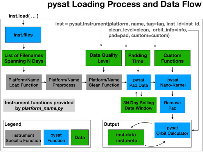
FIGURE 2. Internal pysat data flow when user invokes. Load command.

The ‘init’ method is only called when instantiating the Instrument, and is not shown in the load data flow. The ‘init’ method is generally useful for setting parameters that don’t typically change, such as the data set’s acknowledgements and references. A full Instrument instance is passed to ‘init’ to ensure users and developers can change any aspect of the Instrument.

The ‘preprocess’ function allows a data set plug-in developer to automatically modify loaded data, or an Instrument object, just after the data is loaded internally and before any other changes could be made. This feature is one of the ways developers can transfer their practical data set knowledge to users. As an example, the Communications/Navigation Outage Forecasting System (C/NOFS) IVM (Heelis and Hanson, 1998; de La Beaujardière, 2004; Stoneback et al., 2012) data set begins with measurements at a 2-Hz sample rate but later shifts to a 1-Hz sample rate. The C/NOFS IVM pysat plug-in thus assigns an attribute to the Instrument object during loading for the sample rate. Downstream functions intended for C/NOFS IVM can easily refer to that attribute as needed during processing. Alternately, custom C/NOFS functions can use that information to accurately couple into more general community packages.

After pre-processing, the Instrument object is passed to a ‘clean’ function. This function is written by a developer so that users, by default, operate upon high quality scientific data. While data sets may feature a flag indicating data quality, it is still incumbent upon the user to properly incorporate that flag. For data sets that do not include a quality flag this information may be in a published manuscript, or, in a worst case scenario, not present. Thus the ‘clean’ function allows knowledgeable developers to construct data filters that correspond to four quality levels, ‘clean’, ‘dusty’, ‘dirty’, or ‘none’. By default, data is loaded at the ’clean’ level. This setting may be updated by users, either as a general pysat wide parameter, or when setting up the Instrument.

After cleaning, the Instrument object goes through optional data padding that turns disparate files into a computationally continuous data set. Time based calculations can require a minimum number of continuous samples for proper output. Thus, to apply this function to the first sample of a file could require more samples for an accurate calculation than would otherwise be loaded (such as data before and after the desired analysis period). The data padding feature, enabled at the Instrument level, pads the primary loaded time frame with a user specified amount of data before and after the primary data window. After padding, the data is processed by user specified functions, then the additional padded data is removed. The feature thus provides a user transparent spin-up and spin-down data buffer that produces accurate time-based calculations equivalent to loading the full data set. To minimize excess loading, a cache is employed for leading and trailing data.

The ‘Custom Functions’ section enables users to attach a sequence of user provided functions that will be automatically applied to the Instrument object in order as part of the loading process. This functionality makes it possible to easily modify data as needed for instrument independent analysis code. Suppose there is an analysis package that internally loads one or more days of data. If a user wants that analysis applied to a calculated variable not directly stored in the data set file then without custom functions the user would have to either modify the analysis package to modify the data after it is loaded, or produce a new file that also includes the new data and then use that data set. By including a custom processing queue within the Instrument object data from the file may be arbitrarily modified without requiring any changes within the external analysis code. The only requirements on these functions are that the Instrument object must be the first input argument and that any information to be retained is added directly to the Instrument.

For a standard load call the pysat data flow is now complete. The loaded data is attached to the Instrument object through a ‘data’ attribute, readily available to the user for further modification.

The availability of programmatic hooks at multiple locations within the data flow makes it possible for developers and users to easily configure a data flow that satisfies a broad range of technical and processing requirements.

An additional layer of versatility is supported by enabling users to engage options within Instrument plug-ins. Custom keyword arguments provided by users are identified and passed to appropriate plug-in functions. These keywords only need to be defined in the data set plug-in code. Pysat identifies any undefined keywords in relevant method calls, compares these keywords to those defined in the plug-in methods, and passes matching keywords and values to the relevant methods. These keywords may be provided upon instantiation or in a method call. If provided both at instantiation and in a particular call then the value in the method call is used. The value at instantiation is retained and used by default if a value is not provided in the relevant call.

2.1.5 Iterating through data

Analysis of data over time requires loading data over a range of days, files, orbits, or some general condition upon the data. Pysat includes functionality to support this type of loading through iteration independent of the data distribution in the files. Loading data through iteration engages the same process in Figure 2 to ensure a consistent user experience.

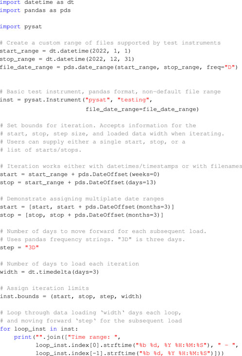
Pysat’s iteration may be accessed using Python’s for loop construction as demonstrated below.

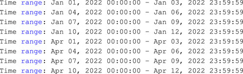
The code produces the following output,

The bounds of the iteration are set through the Instrument ‘bounds’ attribute, which may contain one or more ranges of date/files that the Instrument will load data for. In addition, users can set the number of days/files to load each iteration, as well as the number of days/files to increment for the next iterative load. The bounds attribute is employed, rather than using a specification in the for loop itself, so that iteration independent code may be constructed by developers.

After imports and definition of time ranges, a Instrument is instantiated with a simulated satellite-like test data set. The default range of ‘files’ for the simulated data are outside the desired range so the ‘file_date_range’ custom keyword is used to alter the supported range of dates. Note that the ‘file_date_range’ keyword is specific to the pysat testing data plug-ins and is not a keyword supported for all Instruments. Next, two example definitions for the starting and ending conditions are shown. The bounds are assigned through ‘inst.bounds’ and are followed by the iteration commands.

Each iteration of the for loop will load 3 days worth of data using the ‘inst’ Instrument object. A copy of the ‘inst’ Instrument object is returned as ‘loop_inst’. For performance reasons the underlying data within ‘inst’ is not actually duplicated but is available through ‘loop_inst’. The next loop will step forward ‘step’ days and load ‘width’ days, repeating until the final stop bound is reached.

Users may also iterate through data one orbit at a time. This iteration calculates the locations of orbit breaks as part of the data loading and orbit iteration process. The process enables users to employ arbitrary conditions to define an ‘orbit’. Complete orbits are returned each loop independent of day or file breaks.

The current code has support for identifying orbits through an orbit number variable, a negative gradient, or a sign change. If an orbit value is already provided pysat will iterate through the data set selecting all times with the next orbit value each iteration. The negative gradient or sign change detectors look for specific data conditions with the user supplied data variable to determine where orbit breaks occur.

The orbit iterator can compare the time of a detected orbit against a user supplied value to limit false positives when working with noisy data. Note that some tolerance is required as not all orbit types have a consistent orbit period. Geophysical variability in the orbit environment can physically change orbit properties. Additionally, orbit periods calculated with respect to magnetic local time aren’t consistent orbit to orbit. This variability arises due to the offset of the geomagnetic field with respect to Earth’s rotation axis.

In the future the orbits class will be generalized so that users can directly select a wider variety of techniques for calculating iteration breaks in the data. This generalization in user input will enable iterating through the data against arbitrary data conditions, not just against orbit expectations.

2.1.6 Creating files

Support is included for writing Instrument objects to disk as a compliant netCDF4 file with arbitrary metadata standards. By default, pysat will create files with a simplified version of the Space Physics Data Facility (SPDF) International Solar-Terrestrial Physics (ISTP)/Iteragency Consultancy Group (IACG) standard. Instrument objects may be written to disk, then reloaded, without loss of information.

The Ionospheric Connections (ICON) Explorer mission created a new standard for SPDF and netCDF4 files. The original SPDF standard was composed for Common Data Format (CDF) files. ICON chose the netCDF variant for the mission which required some translation from the original standard due to an existing library of netCDF software. To achieve the greatest software compatibility the SPDF netCDF4 format includes some information under multiple names. For example, the standard itself requires the use of '_FillValue' but 'FillVal' is also mandated for community compatibility reasons. Further, maximum and minimum expected data values have multiple names. To support the SPDF netCDF4 and other formats pysat makes it possible to arbitrarily modify stored Instrument metadata as it is being written to the file. This enables developers to work with the minimum unique information throughout processing and then expand as needed for file creation.

The code below maintains metadata compliance with the full SPDF netCDF4 standard.

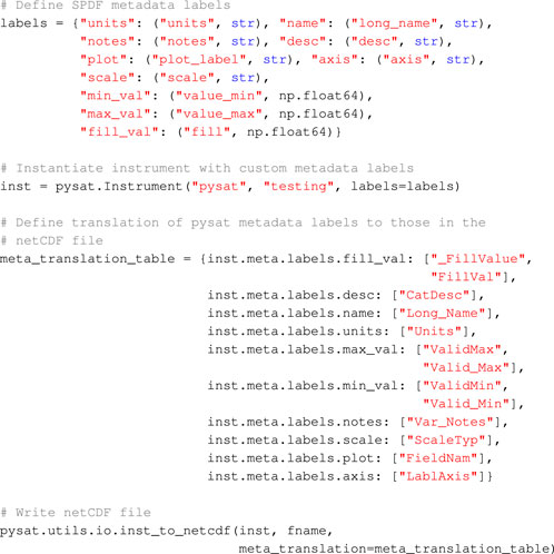
The labels class provides a mapping from the types of metadata to be stored, the string value used to store the metadata, and the default type for that parameter. The labels dictionary is provided at Instrument instantiation to modify the default metadata labels. While the underlying ‘testing’ data set is created with the standard pysat metadata labels, and not the expanded labels needed for SPDF, pysat will automatically translate the standard labels in the file to the user provided values as part of loading. New labels without a corresponding entry in the data are left empty.

The ‘meta_translation_table’ defines a mapping from the metadata labels in the Instrument object to those used when writing a file. Entries may be mapped to one or more labels in the file. The multi-label support is used to convert single entries at the Instrument level, such as the minimum expected data values, to multiple labels in the file, ‘Valid_Min’ and ‘ValidMin’.

Additional parameters required by SPDF but that can be unambiguously determined directly from data are handled by pysat. The time data also has different metadata parameters available and is assigned by pysat. Metadata is constructed in the same way for both xarray and pandas Instrument objects. For pandas objects pysat directly creates the netCDF file. For xarray objects pysat uses xarray’s netCDF4 functions when writing the actual file.

Global attributes in the netCDF4 file created in the code above may be set by assigning new attributes to ‘inst.meta.header’.

2.1.7 General settings

Pysat has a parameters class to create a central location for users to set pysat or custom settings. The ‘pysat.params’ class stores defaults for checking file system every instantiation, default clean level, directories for data, whether to ignore empty files, and registered user modules. Users may also assign their own custom entries.

2.1.8 Constellation

To support the use of multiple data sets in concert pysat also offers a Constellation class. Constellations may be defined and distributed by a developer, similar to Instrument data set plug-ins. Alternately, users can collect an arbitrary group of Instruments in a list to instantiate a Constellation object or create a Constellation of all available Instruments that share a set of defining characteristics (e.g., load all historic ACE data or all instruments from an observational platform). There are no restrictions on the types of Instruments object that may be combined in a Constellation.

The intent of the Constellation class is to provide a high degree of compatibility between Constellation and Instrument objects in terms of attributes and methods. As an example, invoking the Constellation load method will trigger a corresponding call to load data for all Instrument objects within the Constellation. However, as the Constellation object is a collection of Instruments, each Instrument may still be manipulated individually. For example, custom functions may be applied to the Constellation object itself (affecting all Instruments) or to single Instruments within the Constellation.

The Constellation class is more than simply a wrapper for a list of Instruments. It contains several attributes designed to improve analysis on multiple Instruments. These include the establishment of a common time-series and attributes (‘empty’ and ‘partial_empty’) that define if all, some, or no data was present for the desired time period. The Constellation class is the youngest of the core pysat classes, and is undergoing active testing and development. Future enhancements include a method to convert from a Constellation to an Instrument and allowing Constellation sub-modules to provide ‘init’ and ‘preprocess’ methods.

2.2 The penumbra environment

To provide support for the broadest array of data sets and data providers, both in and out of science, pysat is designed to accommodate data sets through a modular system. This system design ensures a consistent user experience without requiring any consistency from data providers or analysis packages. For Python packages built using pysat, the user will (for most processes) call pysat directly. This simplifies the analysis process for scientists performing studies from multiple data sets.

Because the data providers are typically self-consistent, pysat packages that focus on providing data are organized by data provider. pysatNASA (Klenzing et al., 2022b) supports NASA data from Coordinated Data Analysis Web (CDAWeb), pysatMadrigal (Burrell et al., 2021) for National Science Foundation (NSF) data from Madrigal database, and pysatCDAAC (Klenzing et al., 2021) for Cosmic Data Analysis and Archive Center (CDAAC) data. Other pysat packages focus on a particular type of data set that may span multiple data providers: pysatSpaceWeather (Burrell et al., 2022b) focuses on space weather indices and real-time data, while pysatModels (Burrell et al., 2022a) has utilities designed to facilitate model-observation comparisons and loading model files for analysis. Other pysat packages focus on a particular analysis goal, with pysatMissions (Klenzing et al., 2022a) providing tools to simulate and propagate orbits for current or future space missions and pysatSeasons (Klenzing et al., 2022c) providing averaging processes independent of data source and dimensionality.

Template instruments are included in pysat as well as several of the pysat Penumbra packages to make it easier for users and developers to add new Instruments. The templates include calls to pysat provided functions that are generally applicable. Each stage of the template Instrument plug-in is documented with comments and descriptive basic docstrings.

To assist developers in ensuring compliance of data module functions pysat includes a suite of unit tests for external instrument modules. Data modules outside the core package can inherit this core suite of tests in local tests built using pytest (Krekel et al., 2004). These tests cover standards compliance for each module, as well as a test run of a common set of operations: download a sample file, load it with different levels of cleaning, and test remote file listing if available. All test data is downloaded to a temporary directory to avoid altering an end user’s working environment should they contribute to the code. The tests are inherited from a top-level class, and are used across the ecosystem to maintain consistent standards. Additional tests for instruments with custom inputs can be added at the package level using the inherited setup.

2.2.1 Currently supported data

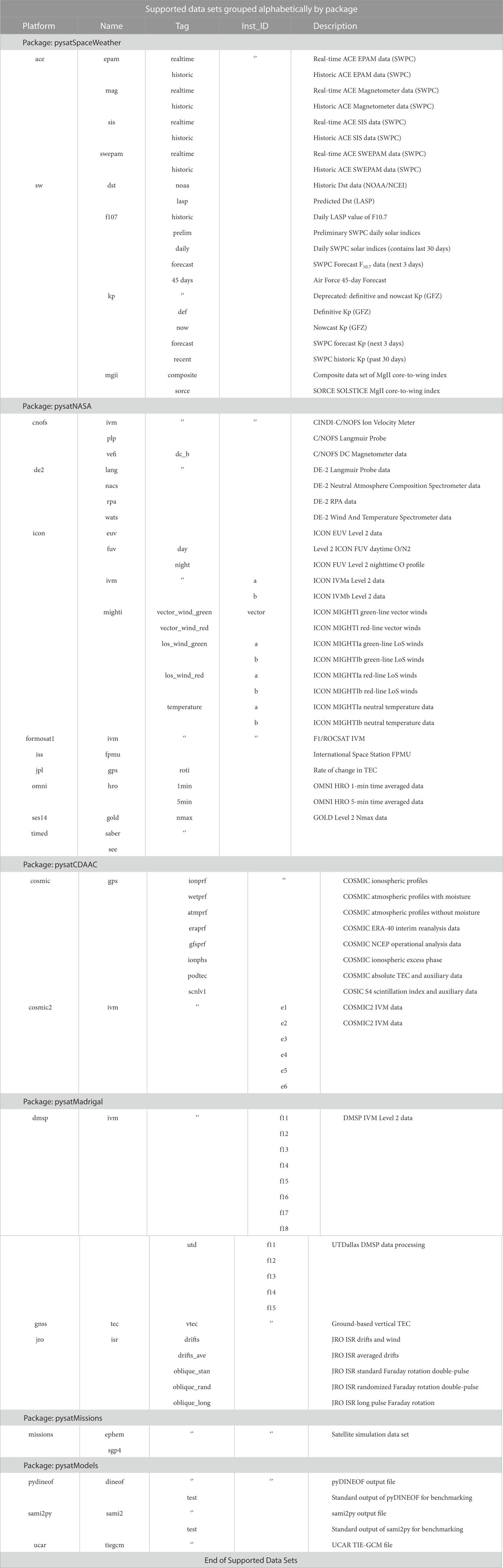
2.2.2 Supporting new data sets

Pysat’s plugin design enables the wider community to load any data set via pysat. Given pysat’s plug-in design, pysat does not directly identify, download, load, or clean a data sets files. Rather, pysat directs Instrument plug-ins, or a collection of appropriately written methods, to perform various actions as required to work with a particular data set.

Pysat has an ionospheric heritage, reflected in the currently supported data sets across the pysat ecosystem, consistent with the scientific focus of the developers. However, pysat itself is not limited to ionospheric or even scientific data. As the pysat team cannot directly develop plug-ins for every data set, pysat is designed so that users can construct their own plug-in modules to support their own particular data. This user available Instrument plug-in creation support is the same used by the pysat team to add the full variety of data sets in section 2.2.1.

In this section we provide an overview of Instrument plug-in requirements and demonstrate that any data set that a user can load on their own system is a data set that can be loaded from the pysat interface. An example for an Instrument support plugin is included below. The docstrings and other comments have been significantly reduced here for brevity. The full template is included with the pysat source code under ‘pysat/instruments/templates‘. The file should be named ‘platform_name.py‘ where ‘platform‘, ‘name‘ are replaced with appropriate values. These identifiers are used by pysat when a user instantiates an Instrument object. The instrument plug-in file must be part of a python module and registered with pysat before it will be available for use.

First, a variety of Instrument attributes are set by the developer, along with a range of testing attributes. Pysat includes a suite of general Instrument plug-in tests that are applied to all registered plug-ins whenever unit tests are run. This is done to make it easy for users to ensure compliance of any plug-in code. The testing attributes enable the developer to specify what types of tests to run and under what conditions.

Following the attribute assignments a variety of required and optional functions are defined. The use of these functions within pysat’s loading process is covered in section 2.1.4. Minimum required functions are ‘list_files‘, ‘load‘, ‘clean‘ and ‘download‘. The ‘preprocess‘ is optionally defined as needed by developers to modify data as it is loaded. Finally, the ‘list_remote_files‘ is optional but recommended. Pysat uses this function to keep a local system up to date with respect to the most recent server data.

The ‘init‘ function is run once upon instantiation. As shown, it is typically used to set references, acknowledgements, and other top-level Instrument attributes. The ‘clean‘ and ‘preprocess‘ functions provide opportunities to clean the data, as requested by the user, or otherwise processes or modify the data before it becomes available to the user. These functions are data set specific. The ‘init‘, ‘clean‘, and ‘preprocess‘ functions all receive the pysat.Instrument object as input.

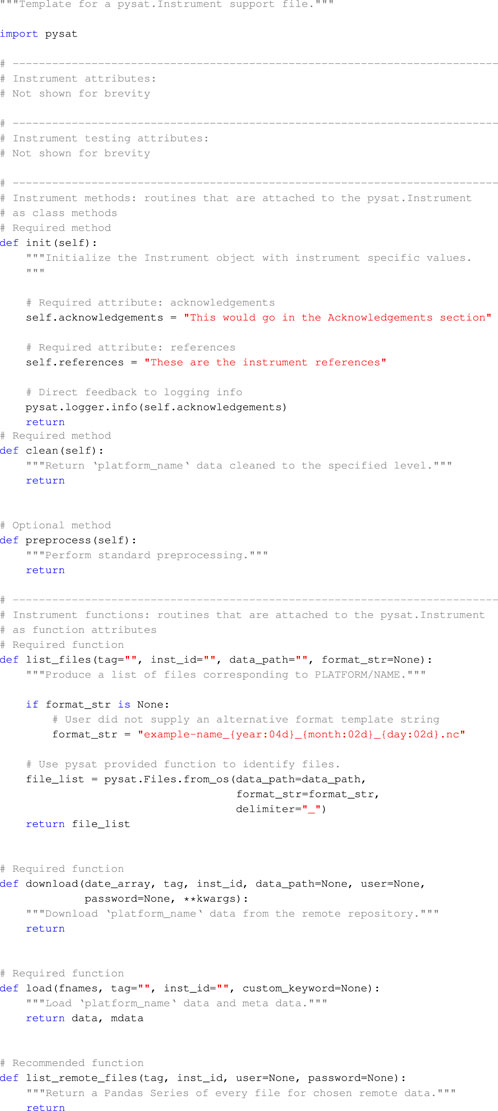
The ‘list_files‘ function provides pysat with information on the files on a user’s system. The function as presented is typically sufficient for most data sets, the developer merely needs to provide a filename template in the variable ‘format_str‘ as well as set keywords in the call to ‘pysat.Files.from_os‘. The ‘format_str‘ variable provides information on which portions of a filename contain relevant information and how to parse that information. The example includes the ‘year‘, ‘month‘, and ‘day‘ keywords, thus the day will be treated as day of month. If only ‘year‘ and ‘day‘ are included then the day is treated as day of year.

The ‘download‘ function is responsible for downloading data for the provided dates in ‘date_array‘ to the local ‘data_path‘ location. User information is provided by the user, as needed, when they invoke the download method. It is up to the developer to provided the underlying functionality to actually download the data. Typically, this function is the same for a given data source provider.

The ‘load‘ method is responsible for loading data from the local system and returning appropriate data and metadata. A list of filenames to be loaded is provided to the developer by pysat. It is up to the developer to provide the required functionality to load the files and suitably format the loaded data and metadata for pysat. Metadata is stored within the pysat.Metadata class to ensure a proper format. Properly formatted data is either a pandas DataFrame or an xarray data set. A given data provider may tend to serve files in a particular format, thus, the load function may be shared across multiple plug-ins from the same source.

Any file format may be loaded with this plug-in design. Note that pysat itself doesn’t impose any requirements on the formatting of the data or the metadata to be loaded, only on the data and metadata returned by the function. For simple text or other data files that don’t include metadata in the file the developer can define the information in the function and return it as part of the metadata. As metadata in pysat is primarily informational the system still functions even when no metadata is provided by a developer though pysat warns the user that metadata defaults are being applied.

While pysat is file format agnostic when loading data, pysat includes built-in support for writing and loading netCDF files. The netCDF support will, by default, transparently store and load an instantiated pysat.Instrument to and from disk. The functions also include a variety of metadata and other options to store the data using other file standards with user specified properties. Support for loading other file formats, Common Data Format (CDF) and Hierarchical Data Format (HDF), may be found in pysat penumbra packages pysatCDF (Stoneback et al., 2022) and pysatMadrigal, respectively.

3 Penumbra examples

3.1 Instrument independent analysis

The pysat Instrument and Constellation objects make it possible to build analysis software that works with any combination of data sets. This generalization removes the need for repeated development or modification of the same analysis functions but applied to different data. Analysis packages built upon pysat can also utilize the included test instruments to develop rigorous unit tests and enable validated access across the community. These features increase the general trustworthiness of manuscripts while simultaneously reducing the workload upon the scientists.

Each of the following sub-sections covers a single pysat example.

3.1.1 Bin averages in time

PysatSeasons generalizes the commonly employed two dimensional binning of data, such as binning a variable over longitude and local time, to produce maps of geophysical parameters. pysatSeasons is built on pysat’s Constellation object to accommodate averaging data from multiple data sets at once. It supports binning N-dimensional data within each bin as all input data is translated into xarray form.

An example producing the distribution of ion density as functions of magnetic local time and longitude using data from the Constellation Observing System for Meteorology Ionosphere and Climate (COSMIC-2) constellation is in the code below.

A user-defined constellation is created after the pysat directory assignment by defining a list containing Instrument objects for each satellite within the six satellite constellation. The list of Instruments is provided to the Constellation class at instantiation. The bounds of the analysis are set at the Constellation level which passes these limits to each individual Instrument object within.

While measurements of ion density are directly available in the COSMIC-2 IVM files, given the large range in values for this analysis we want to produce a map of the log of the density. A simple function to calculate the log of ion density, as well as add appropriate metadata, is defined after the bounds assignment. After definition, this custom function is attached to all the Instruments within the Constellation by attaching the function using the Constellation class ‘custom_attach’ function. Support is also offered for applying custom functions at the Constellation level. Functions must accept a Constellation as the first input rather than an Instrument. Alternately, users may directly attach custom functions to individual Instruments.

Near the end of the example code the pysat logger is updated to provide additional feedback as the pysatSeasons bin averaging process runs. The ‘median2D’ function will load data for each of the Instruments in the Constellation over the assigned bounds, binning the data as appropriate. After all constellation data is loaded a median is applied to the data within each bin. Though the binning function currently only internally supports calculating the bin median, all of the binned data may be returned to the user with the ‘return_data’ keyword, enabling application of any statistical analysis.

The returned output in the final line of code is stored in ‘results’, a dictionary, whose values are plotted in Figure 3. Raw density values range over multiple orders of magnitude thus the observed range in values between 4-5 is clear evidence that user generated variables added through the custom functions features are supported for averaging. Consistent with general geophysical expectations a clear wave three signature is seen in longitudinal variations in total ion density near local noon.

FIGURE 3

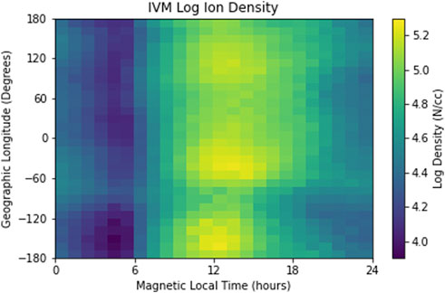
FIGURE 3. Median ion density from COSMIC-2 constellation from January 1—January 31, 2021.

3.1.2 Occurrence probability

PysatSeasons also includes generalized support for determining how often a user determined condition occurs. The occurrence probability is the number of times the condition occurs at least once per bin per load iteration divided by the number of times the Instrument made at least one observation in a given bin per load iteration. The occurrence probability may be calculated using a daily (or longer) load iteration or using the orbit iterator.

The code below calculates and plots how often plasma bubbles will be detected at ICON’s location per orbit.

The first three code groups import required packages as well as register a single NASA data set within pysat. Next, a pysat Instrument is instantiated for the Ion Velocity Meter (IVM) onboard ICON. Two optional features are engaged with the instantiation. Namely, information on identifying orbit breaks in the data, as well as data padding for accurate time-based calculations. Finally, a simple date range is set on the object.

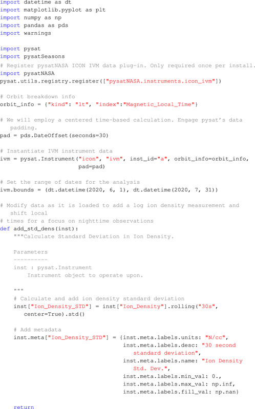
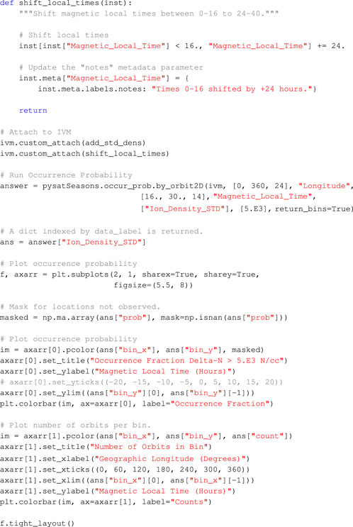
A pair of custom functions are then defined to modify the ICON data as loaded from files. To identify plasma bubbles a simple running standard deviation is defined in ‘add_std_dens’. IVM data is loaded into a pandas DataFrame thus pandas functionality is used to calculate the standard deviation. First, a rolling centered time window of 30 s is defined and that rolling window is used to calculate the standard deviation. Plasma bubbles predominantly occur at night thus the ‘shift_local_time’ function shifts local times from 0 to 24 to 16-40. Both custom functions are attached to the Instrument object.

The occurrence of standard deviations in plasma density greater than 5E3 N/cc as determined by the ‘pysatSeasons.occur_pron.by_orbit2D’ is in Figure 4. The top figure is the distribution of plasma bubbles as a function of longitude and local time, from late afternoon until dawn. Only the South American sector shows any activity. The ‘by_orbit2D’ function uses the pysat Instrument object to iterate through ICON data orbit-by-orbit. In this case, orbit breaks are defined using the ‘Magnetic_Local_Time’ variable and the internally observed locations with significant negative gradients. For complete data sets significant negative gradients would only be observed when local times rolled over from 40 to 16.

FIGURE 4

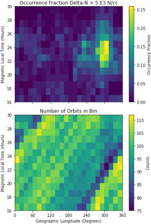
FIGURE 4. Occurrence probability results for ICON IVM between 1 January 2020—31 March 2020.

3.1.3 Model data comparison

PysatModels includes support for loading model data through pysat as well as functionality for comparing model data with other data sets. The code below will download, load, and compare Jicamarca Radar Observatory Incoherent Scatter Radar (JRO-ISR) observations with a test model data set in pysat.

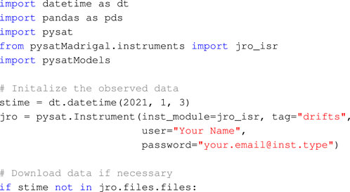
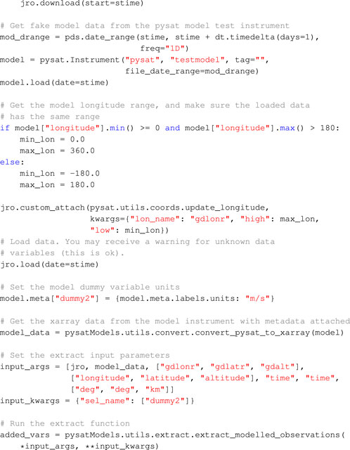
After the imports the JRO instrument is instantiated. Data is downloaded if not already present on the local system. The test model is then instantiated and loaded. The data is simulated thus no download is necessary. To ensure both data sets have the same longitude range, the range from the test model is identified and used as part of the input to a custom function applied to the JRO data, which is then loaded.

Next a comparison between the two data sets is performed. First, for comparison against JRO ion drift measurements a non-specific test variable is modified to have appropriate units. Next, the pysat Instrument object is distilled into an xarray data set. Input arguments identifying equivalent variables between data sets and other needed parameters are constructed and used to extract model-data pairs, locations where both data sets have information. Figure 5 plots the distribution of points for the model, for JRO, and indicates which points are selected as present in both data sets. The values extracted in this case only refer to simulated test data and thus aren’t shown.

FIGURE 5

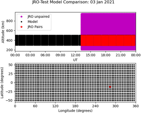
FIGURE 5. Distribution of points identified as part of comparison.

3.1.4 Model data interpolation

PysatModels also includes support for interpolating model data onto another data set. This feature may be used to switch a model to a different grid, or alternately, could be used to project model results onto a satellite orbit.

The code below is an example for interpolating model data from a regular grid onto a satellite orbit.

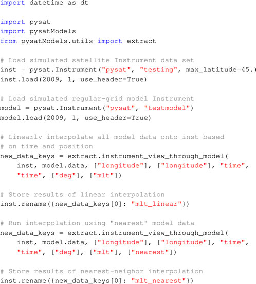
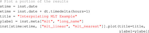
After the imports a test satellite and a test model are both instantiated and loaded with data. Next the model results are interpolated onto the satellite track using either the nearest valid value or a linearly interpolated value. Figure 6 shows a results comparison for both settings. As expected, the linear interpolation produces a smooth signal while the nearest neighbor method shifts between discrete values as the satellite moves and the nearest neighbor shifts.

FIGURE 6

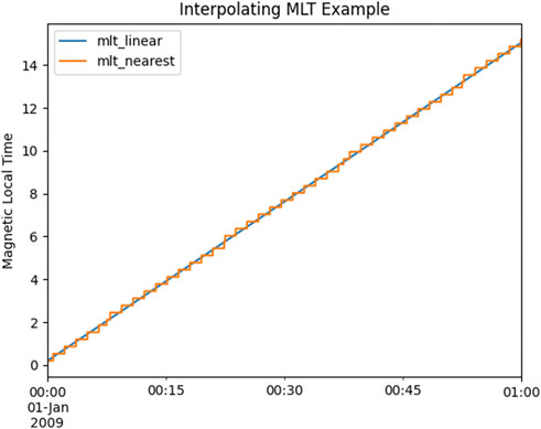
FIGURE 6. One dimensional example for interpolating model data values onto instrument using linear or nearest neighbor interpolation.

Not all models have a regular distribution of points over the variables of scientific interest. The ’pressure_levels’ tag for pysat’s testmodel simulates a model that has a regular grid over longitude, latitude, and pressure level, but pressure level has an irregular relationship to altitude. Interpolating from this model onto a satellite data set with altitude, with performance, requires converting the satellite altitude to a model pressure.

The code below covers the full process.

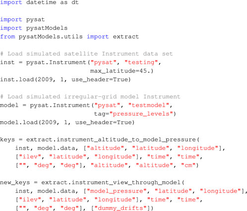
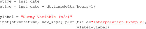
The altitudes and pressure levels in the model are used to generate equivalent pressure levels for the satellite consistent with the satellite altitude through the ‘extract.instrument_altitude_to_model_pressure’ function. The appropriate satellite pressure levels are generated by guessing initial solutions and then iteratively using a regular grid interpolation on the model to get the equivalent altitudes. The satellite pressure levels are increased/decreased as appropriate and the iteration continues until the difference between the actual satellite altitude and the equivalent altitude are within the specified tolerance. The final pressure levels are stored as ‘model_pressure’ in the satellite Instrument.

The obtained satellite pressure is used with regular linear interpolation to extract model ion drift values along the satellite track through the ‘extract.instrument_view_through_model’ call. The resulting interpolated quantities are accurate and generated much faster than using a full irregular interpolation, available through ‘extract.interp_inst_w_irregular_model_coord’. The results of the interpolation are in Figure 7.

FIGURE 7

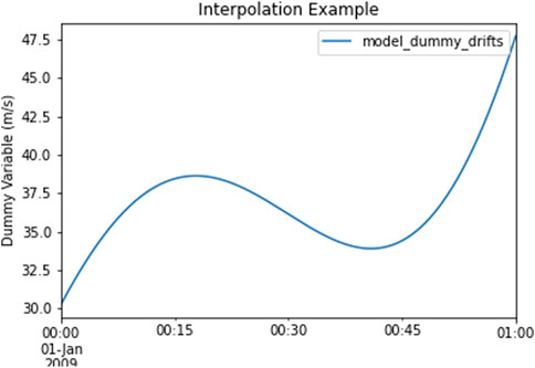
FIGURE 7. Interpolating irregularly gridded data in altitude onto Instrument using intermediate pressure calculation to enable regular interpolation.

3.2 Satellite instrumentation processing

The file management, data, and metadata features within pysat are well suited for science instrument data processing. Scientific instrumentation goes through a general data flow. Raw measurements directly from the instrument are converted to physical quantities. These physical measurements are then used to generate geophysical parameters such as ion density or temperature. Finally, the results are stored in standards compliant files and distributed to the public.

While the details of created files, and the instruments themselves, may vary from mission to mission, building instrumentation processing on pysat makes it easy to build long term heritage in processing while still being versatile and adaptable. IVM processing software for ICON and COSMIC-2 is built on pysat. First, A general IVM processing package was developed. The functions within were written using the pysat Instrument object to provide access to needed data and metadata. A higher-level package was then created for both ICON and COSMIC-2 that simply connects the generalized IVM processing package with the ICON and COSMIC-2 processing environments and file standards. This design configuration ensures that any processing improvements developed or identified within a single mission are automatically available for the other missions. It further allows for significant unanticipated differences between instruments as well as processing environments without modifying the core software.

Unit tests were developed for the generalized IVM package based upon the simulated pysat test instruments. Since the package was built on pysat, it is easy to substitute new data sources into the processing, simulated or measured. These unit tests may thus be reused for future missions, saving future developer time, and ensuring that processing results maintain accuracy across missions.

Using pysat as a foundation makes it easier to deal with unanticipated changes in processing as a mission evolves. This is best achieved by creating a pysat data plug-in that supports each file stage during processing. This enables pysat to mediate loading data as well as provides access to a variety of mechanisms to alter data as needed. The plug-in structure provides multiple functional hooks for working with the data under a variety of conditions. Further, the custom function queue attached to the Instrument makes it easy to change that processing as the mission evolves. For a Constellation object, the functional hooks make it easy to alter the processing of some Instruments within the Constellation. The performance of the same physical instrument may not be the same across an actual constellation of satellites.

3.2.1 Satellite ephemeris

In addition to analysis of existing satellite data, one can also build simulated spacecraft orbits through the pysatMissions package. The core instrument module here simulates a day of orbits using the sgp4 (Rhodes, 2018) package. The spacecraft can be generated from either a pair of Two-Line Elements (TLEs), or from a set of individual orbital elements (orbital inclination, altitude of apoapsis, etc.). When combined with pysatModels simulated data can be added to the simulated orbits. While the data is generated on the fly, operations and analysis are identical to a standard pysat instrument. The current accuracy of the simulated orbit is on the order of 5 − 10 km in altitude for low Earth orbits. Improvements to the accuracy are planned in the future.

The code below uses pysatMissions to simulate a satellite orbit as well as iterate through the simulated data set, orbit-by-orbit.

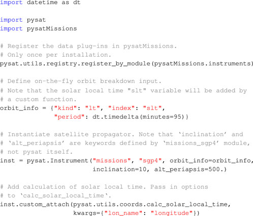
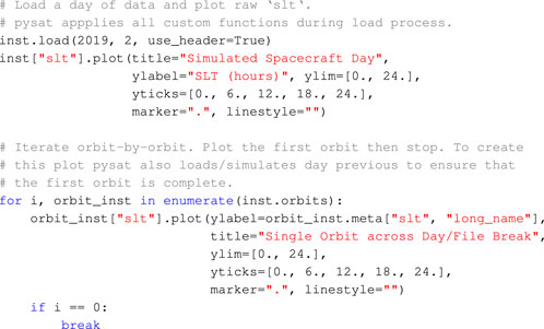
After the imports and pysat directory assignment, a dictionary is defined with information needed by the pysat orbit iterator to determine orbit breaks on the fly. The ‘index’ identifies the variable for the system to use, while ‘kind’ selects between several internal orbit break calculations, in this case local time. The period sets the nominally expected orbit period. The subsequent input cell uses this information as part of instantiation. Multiple parameters used internally by the orbit propagator are also set. Internally, these keywords are routed to the appropriate ‘missions_sgp4’ plug-in function.

A calculation of solar local time within pysat is coupled to the simulated orbit using the ‘inst.custom_attach’ command. The function itself simply passes user identified variables into the relevant pysat call, then adds the output variables to the Instrument, with metadata. Not all Instrument data sets label quantities like longitude, latitude, or altitude the same, thus string inputs are used to accommodate different naming schemes. Note that only the label to access the data, not the underlying data itself, is passed so that the process works as part of the load process for any day or combination of days.

Data for 2 January 2019 is simulated and loaded into the Instrument object through the standard ‘inst.load’. The full data set is plotted in Figure 8 to demonstrate that the simulated orbit data is treated in the same way as typical satellite data. Note that the first sample is from January 2.

FIGURE 8

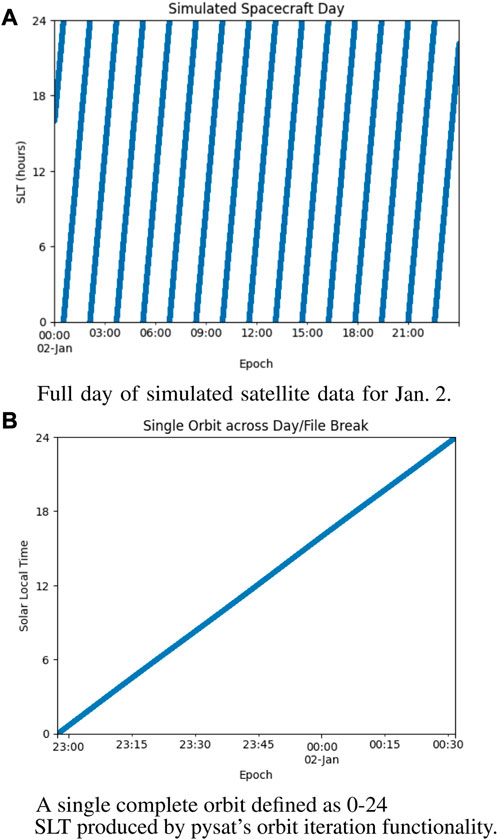
FIGURE 8. (A) Full day of simulated satellite data for January 2 (B) A single complete orbit defined as 0-24 MLT produced by pysat’s orbit iteration functionality. Note the orbit begins on January 1 and ends on January 2, spanning two files. Replace with fancier ICON summary type plot!.

Finally, pysat’s orbit iteration is used to break down the daily increment of loaded satellite data into individual orbits. In this case, orbit breaks are determined using solar local time, appropriate for plasma investigations due to the large influences from the Sun and the geomagnetic field. The code is configured to stop the for loop after the first orbit is loaded. The intent of the orbit iteration is to provide full orbits each increment of the iteration loop. As orbit boundaries generally do not respect file or day breaks, pysat uses its internal data cache to load and store data from January 1 as part of its internal calculations. Thus the first orbit sample at 0 Solar Local Time (SLT) occurs on January 1. Note that the load statement from the previous cell is not required for the iteration, orbit or otherwise, to function.

4 Conclusion

The abstractions and functionality provided by pysat enables it to integrate a wide variety of data sets and analysis tools, current or historical, into a cohesive whole. This is particularly important for historical packages that are unlikely to comply with current or future data file standards, since pysat does not impose any requirements upon these external packages. The versatility of pysat’s coupling functionality also addresses a fundamental challenge in open source development. Due to the low barrier for open source development there are a wide variety of packages in the scientific community. However, by being open there is no specific requirement that these packages all work together. Of course, with specific effort individual packages may be coupled on a one to one basis. With pysat though, each coupled package coupled is now in an ecosystem where the outputs from the other packages are also available, creating a one to many coupling.

The versatility of pysat’s design enables scientists and developers to address the unique aspects of any instrument while retaining a systematic and coherent structure. For each type of change desired by a user, or developer, pysat has built-in functionality to mediate that change. Pysat is thus also well suited as a foundation for instrumentation processing. The plug-in design supports the development of robust and verifiable code for instrumentation processing. Further, the attention to the full data life cycle ensures full support for metadata and the requirements of creating publicly distributed files.

Data availability statement

Publicly available datasets were analyzed in this study. This data can be found here: https://github.com/pysat/.

Author contributions

RS, AB, and JK are core pysat developers. JS is a regular pysat contributor. RS is the primary author of the manuscript. RS, AB, JK, and JS edited and reviewed the manuscript. All authors read and approved the manuscript for submission.

Funding

This work was supported by the DARPA Defense Sciences Office. RS was supported by the Naval Research Laboratory, N00173191G016 and N0017322P0744. AB is supported by the Office of Naval Research. JK was supported through the Space Precipitation Impacts (SPI) project at Goddard Space Flight Center through the Heliophysics Internal Science Funding Model. JS supported through NNH20ZDA001N-LWS and 80NSSC21M0180.

Conflict of interest

The authors declare that the research was conducted in the absence of any commercial or financial relationships that could be construed as a potential conflict of interest.

Publisher’s note

All claims expressed in this article are solely those of the authors and do not necessarily represent those of their affiliated organizations, or those of the publisher, the editors and the reviewers. Any product that may be evaluated in this article, or claim that may be made by its manufacturer, is not guaranteed or endorsed by the publisher.

References

Barnum, J., Masson, A., Friedel, R. H., Roberts, A., and Thomas, B. A. (2022). Python in heliophysics community (pyhc): Current status and future outlook. Adv. Space Res. 2022. doi:10.1016/j.asr.2022.10.006

CrossRef Full Text | Google Scholar

Burrell, A. G., Halford, A., Klenzing, J., Stoneback, R. A., Morley, S. K., Annex, A. M., et al. (2018). Snakes on a spaceship—An overview of python in heliophysics. J. Geophys. Res. Space Phys. 123, 10384–10402. doi:10.1029/2018JA025877

CrossRef Full Text | Google Scholar

Burrell, A. G., Klenzing, J., Stoneback, R., and Pembroke, A. (2021). pysat/pysatmadrigal. v0.0.4 release. doi:10.5281/zenodo.4927662

CrossRef Full Text | Google Scholar

Burrell, A. G., Klenzing, J., Stoneback, R., Pembroke, A., Spence, C., and Smith, J. M. (2022b). pysat/pysatspaceweather. v0.0.7. doi:10.5281/zenodo.7083718

CrossRef Full Text | Google Scholar

Burrell, A. G., Klenzing, J., and Stoneback, R. (2022a). pysat/pysatmodels. v0.1.0 release. doi:10.5281/zenodo.6567105

CrossRef Full Text | Google Scholar

de La Beaujardière, O. (2004). C/nofs: A mission to forecast scintillations of equatorial aeronomy sparked by the Jicamarca radio observatory. J. Atmos. Solar-Terrestrial Phys. 66, 1573–1591. doi:10.1016/j.jastp.2004.07.030.40

CrossRef Full Text | Google Scholar

Harris, C. R., Millman, K. J., van der Walt, S. J., Gommers, R., Virtanen, P., Cournapeau, D., et al. (2020). Array programming with NumPy. Nature 585, 357–362. doi:10.1038/s41586-020-2649-2

PubMed Abstract | CrossRef Full Text | Google Scholar

Heelis, R. A., and Hanson, W. B. (1998). “Measurements of thermal ion drift velocity and temperature using planar sensors,” in Measurement techniques in space plasmas: Particles. Editors R. F. Pfaff, E. Borovsky, and T. Young (AGU), 61–71. doi:10.1029/GM102

CrossRef Full Text | Google Scholar

Hoyer, S., Roos, M., Joseph, H., Magin, J., Cherian, D., Fitzgerald, C., et al. (2022). xarray. doi:10.5281/zenodo.7195919

CrossRef Full Text | Google Scholar

Klenzing, J., Stoneback, R., Burrell, A. G., Depew, M., Spence, C., Smith, J. M., et al. (2022a). pysat/pysatmissions, 3. Version 0.3. doi:10.5281/zenodo.7055089

CrossRef Full Text | Google Scholar

Klenzing, J., Stoneback, R., Burrell, A. G., Smith, J., Pembroke, A., and Spence, C. (2022b). pysat/pysatnasa. v0.0.4. doi:10.5281/zenodo.7301719

CrossRef Full Text | Google Scholar

Klenzing, J., Stoneback, R., Pembroke, A., Burrell, A. G., Smith, J. M., and Spence, C. (2021). pysat/pysatcdaac. Version 0.0.2. doi:10.5281/zenodo.5081202

CrossRef Full Text | Google Scholar

Klenzing, J., Stoneback, R., Spence, C., and Burrell, A. G. (2022c). pysat/pysatseasons. v0.2.0. doi:10.5281/zenodo.7041465

CrossRef Full Text | Google Scholar

Krekel, H., Oliveira, B., Pfannschmidt, R., Bruynooghe, F., Laugher, B., and Bruhin, F. (2004). pytest 7, 2.

Moigne, J. L. (2018). Distributed spacecraft missions (dsm) technology development at NASA Goddard Space Flight Center. IGARSS 2018 - 2018 IEEE Int. Geoscience Remote Sens. Symposium 293–296. doi:10.1109/IGARSS.2018.8519065

CrossRef Full Text | Google Scholar

Pandas development team (2022). pandas-dev/pandas: Pandas. doi:10.5281/zenodo.7223478

CrossRef Full Text | Google Scholar

Pembroke, A., DeZeeuw, D., Rastaetter, L., Ringuette, R., Gerland, O., Patel, D., et al. (2022). Kamodo: A functional api for space weather models and data. J. Open Source Softw. 7, 4053. doi:10.21105/joss.04053

CrossRef Full Text | Google Scholar

Rhodes, B. (2018). python-sgp4.

Stoneback, R. A., Burrell, A. G., Klenzing, J., and Depew, M. D. (2018). Pysat: Python satellite data analysis toolkit. J. Geophys. Res. Space Phys. 123, 5271–5283. doi:10.1029/2018JA025297

CrossRef Full Text | Google Scholar

Stoneback, R. A., Davidson, R. L., and Heelis, R. A. (2012). Ion drift meter calibration and photoemission correction for the c/nofs satellite. J. Geophys. Res. Space Phys. 117. doi:10.1029/2012JA017636

CrossRef Full Text | Google Scholar

Stoneback, R. A., Depew, M., Klenzing, J., Iyer, G., Pembroke, A., Starr, G., et al. (2022). pysat/pysatCDF: v0.3.2 (v0.3.2). Zenodo. doi:10.5281/zenodo.1217180

CrossRef Full Text | Google Scholar