Chromospheric thermodynamic conditions from inversions of complex Mg II h & k profiles observed in flares

1 Introduction

A flare is the release of magnetic energy as a consequence of reconnection in magnetically stressed coronal loops. The magnetic energy stored in these loops comes from the low solar atmosphere. Once it is released, it is transferred to both the outer and the lower solar atmosphere in a variety of energy forms: radiation, thermal energy, kinetic energy associated to non-thermal phenomena (accelerated particles and turbulence), magnetic energy (large-scale Alfvén waves), and others. The most evident observational counterpart of this sudden release of energy is an enhancement in the specific intensity in almost any spectral range. This description, although simplistic, allow us to picture the basic flare phenomena. Many complex physical processes however occur and need to be properly studied for a full understanding of this type of solar event. This complexity is also reflected in the observational data we have of flares.

In the last few decades, with the advance of instrumentation, especially instrumentation onboard space-based observatories, we have largely improved our access to a steady flow of high-quality flare data. In this paper, we focus our attention on the interpretation of the thermodynamics conditions during the maximum of the X1.0-class flare of SOL2014-03-29T17:48 (see Figure 1). To this aim, we have inverted the Mg II h&k and C II 1334 & 1335 Å lines observed by the Interface Region Imaging Spectrograph (IRIS, De Pontieu et al., 2014).

FIGURE 1

FIGURE 1. Panel (A) Temporal evolution of the X-ray flux during the X1-class flare at SOL2014-04-29T17:48. The vertical lines indicate the number of some IRIS rasters that recorded this flare. Panel (B) The image taken by the SJI instrument at IRIS during the maximum of the X1-class flare SOL2014-03-20T17:48 at 2796 Å, that corresponds to the chromosphere. The time indicated at the top of the panel corresponds to the step number 4 of the raster. The location of the slits of all the steps of this raster (no. 175) are indicated with vertical lines. The colored squares mark the location of the extremely pointy profiles of the type A (blue) and the type B (orange), and of the very pointy or combined profiles (green). The locations in dark colors correspond to the profiles shown in Figures 3–5 respectively. The grey rectangle delimits the area shown in Figure 14.

The resonance Mg II h&k profiles have been used in the past for the study of the chromosphere (Lemaire and Skumanich, 1973; Kohl and Parkinson, 1976; Kneer et al., 1981; Lites and Skumanich, 1982), including the study of flares (Lemaire et al., 1984). The theoretical modeling and interpretation of these lines have been an active topic for decades (e.g., Feldman and Doschek, 1977; Lites and Skumanich, 1982; Lemaire and Gouttebroze, 1983; Uitenbroek, 1997). More recently, thanks to the advance in the computational resources and triggered by the huge amount of data provided by IRIS, these lines have been investigated using more realistic assumptions when solving the radiative transfer equation (RTE) (e.g., Leenaarts et al., 2013a; Leenaarts et al., 2013b; Pereira et al., 2013; Pereira et al., 2015; Sukhorukov and Leenaarts, 2017), including treatment of polarized radiation (del Pino Alemán et al., 2016; Manso Sainz et al., 2019). Kerr et al. (2019a) and Kerr et al. (2019b) have investigated the effect of the physics included in the radiation transport to forward-model these Mg II h&k lines from radiative hydrodynamic flare simulations. These authors conclude that to properly reproduce these lines we need to consider: i) partial frequency redistribution of the scattered photons (PRD), ii) only hydrogen and Mg II need to be included in non-local thermodynamic equilibrium (non-LTE), iii) nonequilibrium hydrogen populations, with nonthermal collisional rates, iv) an atom model with more levels than the ones involving the resonance Mg II h&k lines, and v) the irradiation from hot, dense flaring transition region, which can affect the formation of Mg II. Kerr et al. (2019b) also suggest to consider the nonequilibrium (NEQ) ionization when the atomic level populations are calculated, instead of the statistical equilibrium (SE), for most of the stages of the flare. However, these authors also acknowledge the computational cost of considering this approach, and for most of the duration of the flare, especially the stronger ones, the SE approach is valid. Nevertheless, a careful treatment of the hydrogen lines and the electron densities, prior the calculation of the Mg II h&k lines, is also important for the proper synthesis of these lines, as (Liu et al., 2015) have demonstrated.

The formation and behavior of the C II 1334 & 1335 Å have been investigated by Rathore and Carlsson (2015) and Rathore et al. (2015). Using state-of-the-art numerical models and the most advanced radiative transfer methods, these authors found that these lines can behave as optically thick or as optically thin, and the range of the temperature and height where they are formed can vary significantly, from 6 to 40kK, i.e., from the chromosphere to the transition region.

In this work, we have analyzed the profiles of these lines corresponding to the flare ribbons during the maximum of the flare. In this location, at that time, the Mg II h&k profiles are characterized by a pointy, broad-on-the-base shape¹. Figure 2 shows a typical Mg II h&k profile in the quiet Sun. The main features of the lines and their rest wavelength positions are indicated by labels and vertical lines respectively. In each of these lines, we can distinguish two peaks (the k_2v,r and h_2v,r features) and a central depression or self-reversal in the core of the lines (the k₃ and h₃ features). However, in the profiles studied in this investigation the central depression has disappeared and the top of the profiles is defined by an inverted-V shape in just a few spectral samples. Note that some authors refer to single-peaked Mg II h&k profiles as those profiles that show k₃ and h₃ in emission, but at the same intensity or slightly higher or lower than the k₂ and h₂ spectral features. Such profiles, while being single-peaked, are mostly characterized by being flat-topped, as they were described by Carlsson et al. (2015). The central depression is also reduced when high coronal pressures (10–100 dyn cm⁻²), associated to chromespheric evaporation, are considered (Liu et al., 2015). In contrast, the Mg II h&k profiles discussed in this paper are single-peaked as well, but their main characteristics are: i) their very pointy top, as a consequence of the lack of k₃ and h₃ features and of having the violet and red components of the k₂ and h₂ almost totally blended in one pointy feature, ii) extended broad wings, which renders indistinguishable the k₁ and/or h₁ spectral features; and iii) the subordinated Mg II UV triplet lines are in emission, often also showing a pointy, broad shape, albeit not as extremely pointy, since the top of these lines shows an inverted-U shape.

FIGURE 2

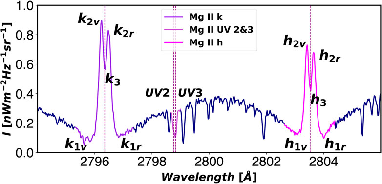
FIGURE 2. Mg II h&k and Mg II UV2&3 lines - the latter belonging to the Mg II UV triplet - as observed by IRIS in the quiet-sun. Spectral sampling is 0.025 Å. The rest position for the core of the lines is indicated by the vertical dashed lines. The main features of the h and k lines are indicated with labels. The wavelength values are given in vacuum wavelength.

The C II 1334 & 1335 Å lines also show a pointy shape, and in many cases, it is red-shifted or showing a strong red-shifted component. These extreme profiles are difficult to invert, and, therefore, the interpretation of the results at values with optical depth log(τ)$<-6.5$ presented in this investigation has to be carefully considered.

Because of this pointy aspect, we refer to these profiles as extreme and very pointy profiles (see Figures 3, 4), and to an intermediate case as combined pointy profile (see Figure 5). A more detailed explanation of this classification is given in Section 2.2.

FIGURE 3

FIGURE 3. Examples of the type A extremely pointy profiles. Panel (A) shows the C II 1,334 & 1,335 Å lines, panel (B) the Mg II UV1 line, and panel (C) the Mg II UV triplet lines, including the Mg II UV2&3 between them. The dashed vertical lines indicate the rest wavelength of these lines.

FIGURE 4

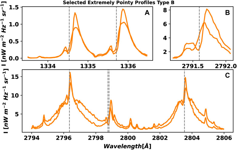
FIGURE 4. Examples of the type B extremely pointy profiles. See caption of Figure 3 for details.

FIGURE 5

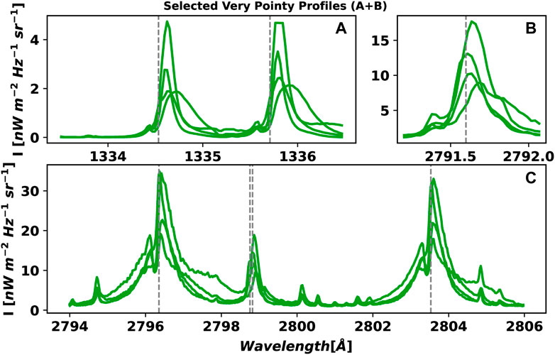
FIGURE 5. Examples of the combined type of pointy profile. See caption of Figure 3 for details.

These kinds of pointy spectral line profiles, especially the Mg II h&k, were identified in IRIS data as soon as the instrument started to observe flares. Kerr et al. (2015) reported strong emission in the Mg II h&k and the Mg II UV2&3 lines in the ribbons of the M class flare SOL2014-02-13T01:40 observed by IRIS. The authors noted the absence of the depression in the core of the Mg II h&k lines, i.e., the lack of the k₃ and h₃ features. They also concluded, based on the ratio of the intensity between the k and the h lines, that these lines are optically thick during the flare. As we just mentioned above, this may not be the case for the C II 1334 & 1335 Å lines. The profiles shown by Kerr et al. (2015) are inverted-U pointy profiles. Figure 6 in Liu et al. (2015) shows a selection of Mg II h&k profiles belonging to the flare studied in the current paper. As we will discuss later, some of the profiles shown in that figure are pointy profiles. Xu et al. (2016) identified extremely pointy Mg II h&k and C II 1334 & 1335 Å profiles in the positive polarity part of the ribbon of the M1.4-class SOL2013-08-17T18:43 flare, but not in the negative polarity part (decrease in the contrast of the intensity).

FIGURE 6

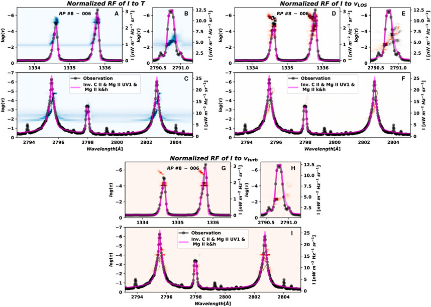
FIGURE 6. Response functions of the intensity (I) to the temperature [panels (A–C)], the v_los(D–F), and the v_turb(G–I) for the atmosphere model corresponding to the extremely pointy profile type A shown in Figure 7 are shown in the background of the panels. The pointy profile and the fit are over-plotted as a reference.

FIGURE 7

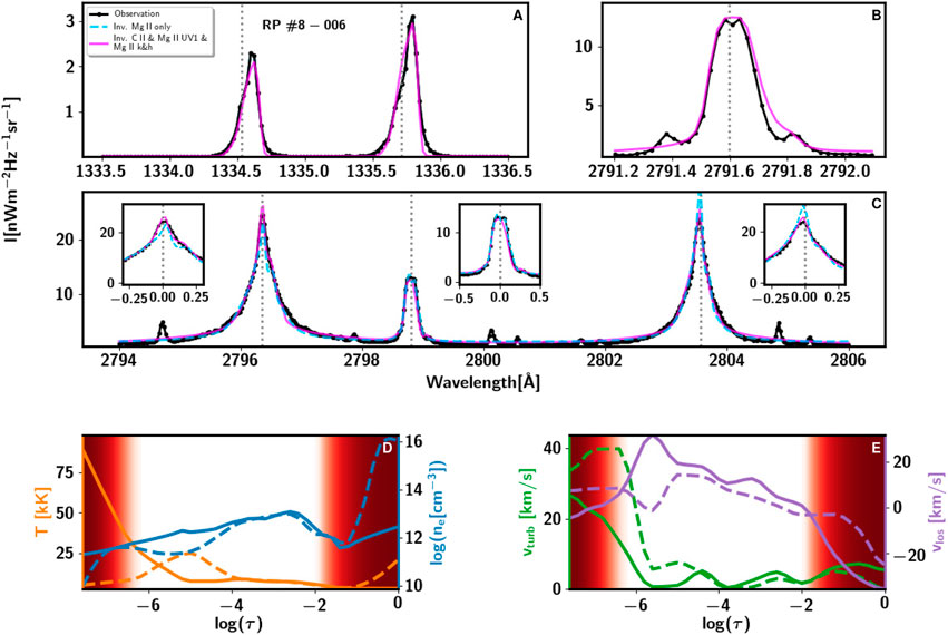
FIGURE 7. Inversion (fit) of the C II 1334 & 1335 Å panel (A), Mg II UV1 (B), Mg II h&k [(C) and left and right sub-panels in panel (C)], and Mg II UV2&3 [(C) and center sub-panel in panel (C)] lines of an extremely pointy profile type A, and the model recovered from the inversion. The three first panels show the inversion of an extremely pointy profile type A (in dotted, black line). The dashed, blue line corresponds to the inversion only taking into account the Mg II h&k lines. The fuchsia line corresponds to the inversion considering simultaneously the C II 1,334 & 1,335 Å lines, the Mg II UV1 line, and the Mg II h&k lines - including the Mg II UV2&3 lines. The last two panels show the thermodynamic variables obtained from the inversions: temperature (T, in orange), logarithm of the electron density (n_e, in blue), velocity of turbulent motions or micro-turbulence (v_turb, in green), and line-of-sight velocity (v_los, in violet). The dashed lines correspond to model recovered from the inversion considering only the Mg II h&k lines, while the solid lines correspond to the inversion considering all the spectral lines mentioned above. The red shade areas in the model atmosphere panels (D,E) indicates the optical depth range that we should not consider as reliable.

Several models have been proposed to explain the pointy profiles, particularly the ones observed by IRIS on SOL2014-03-29T17:48. Rubio da Costa et al. (2016) and Rubio da Costa and Kleint (2017) studied the parameters needed to model the Mg II h&k profiles observed during the maximum of this flare. The authors modified the thermodynamics parameters in hydrodynamic simulations (RADYN, Carlsson and Stein, 1995; Carlsson and Stein, 1997; Allred et al., 2015), and then they obtained the synthetic profiles of these lines using the RH code (Uitenbroek, 2001) considering non-LTE and PRD. The authors obtained inverted-U, single Mg II h&k profiles by increasing the temperature and density in the formation region of these lines. However, the intensity of these profiles is larger than the intensity in the observed profiles. They were only able to match intensity profiles with inverted-U, single-peak profiles when they considered a strong gradient in the line-of-sight velocity (v_los). These calculated profiles show however a significant asymmetry. In addition, their calculated profiles were not able to properly reproduce the large broad wings observed in the IRIS observations, except when they introduced micro-turbulent velocities (v_mic) values as large as 40 km s⁻¹, which they considered to be an unrealistic value. Zhu et al. (2019) followed a similar approach to that of Rubio da Costa et al. (2016), i.e., forward modeling using RADYN and RH, to interpret the Mg II h&k lines of the same flare studied by Rubio da Costa et al. (2016) and Rubio da Costa and Kleint (2017), and by us in the current paper. In this case, the authors considered the impact of the Stark effect on line broadening. They used the STARK-B database - in which line broadening is calculated based on a semi-classical impact-perturbation theory Dimitrijević and Sahal-Bréchot (1995; 1998)–for the treatment of the quadratic Stark effect by RH. This is because the Stark effect was previously implemented in RH considers the adiabatic approximation to calculate the quadratic Stark effect, and this approximation may underestimate the broadening for the Mg II h&k lines during flares (Rubio da Costa and Kleint, 2017). In summary, Zhu et al. (2019) were able to fit the extremely pointy Mg II h&k profiles observed by IRIS in the flare but only by considering an ad hoc contribution of 30 times of the quadratic Stark effect obtained by using STARK-B in RH. This ad hoc assumption allowed them to properly fit the very broad wings of these profiles. However, the authors were unable to provide a physical justification for the large ad hoc enhancement of the Stark effect. They also tried to fit the broad wings by considering the STARK-B database value and various values of v_turb. They found an unrealistic value of v_turb$\approx 30$ km s⁻¹ below the formation region of the line core of the Mg II h&k lines, and even in this case, the fit in the part of the wings furthest from line core is not good both for Mg II h&k and the Mg II UV triplet. In this paper, we focus our attention on the study of both the extremely pointy and the very pointy profiles observed by IRIS during the maximum of the flare. This kind of profile is mostly present during the maximum of the flare. We note that while single-peaked profiles can also be seen in the pre-flare stage and they may help us to predict the flare onset with about 30–50 min advance notice (Panos et al., 2018; Woods et al., 2021), these are quite different: the peak of the latter Mg II h&k profiles shows an inverted-U shape, the Mg II UV triplet is barely in emission, and the C II 1334 & 1335 Å lines show a wide inverted-U shape. The thermodynamics along the optical depth of pre-flare profiles was for the first time described by Woods et al. (2021). In contrast, in the current investigation, we will reveal the thermodynamics of the most intriguing and peculiar profiles emitted at the maximum of the flare.

The interpretation of these extremely pointy profiles during the maximum of flares has presented a challenge for modelers and observers. In this paper, we present a solution - in good agreement with several possibilities speculated in previous work—that is able to reproduce these complex profiles. This solution provides reasonable values of the thermodynamics parameters involved in the problem, i.e., gives a realistic view of the conditions in the chromosphere of flare during its maximum.

2 Materials and methods

The data analyzed in this paper correspond to the maximum of the X1-class flare at SOL2014-03-29T17:48. This data are part of the multi-instrument observations that we led from the Dunn Solar Telescope at Sacramento Peak Observatory in coordination with IRIS and Hinode (Kosugi et al., 2007). Moreover, this flare was simultaneously observed by other observatories such as the Reuven Ramaty High-Energy Solar Spectroscopic Imager (RHESSI, Lin et al., 2002), the Solar Dynamics Observatory (SDO, Pesnell et al., 2012), and the Solar Terrestrial Relations Observatory (STEREO, Kaiser et al., 2008). A description of this unique observation and the evolution of the flare is provided by Kleint et al. (2015), and of the observed Mg II h&k lines by Liu et al. (2015) and Rubio da Costa et al. (2016).

The rasters obtained by IRIS of the region where this flare occurred - NOAA AR 12017—span from 2014-03-29T14:09:39 UT to 2014-03-29T17:54:16 UT. This active region was located at μ = 0.78, with μ = cos θ, and θ the heliocentric viewing angle. The maximum X-ray flux measured by GOES-15 during the flare took place at 2014-03-29T17:48, which corresponds to raster no. 175 of the series of rasters taken by IRIS (see Figure 1). Each raster consisted of an 8-step scan with the slit crossing the two ribbons of the flare. Each step of the raster is 2″ in the direction perpendicular to the slit, covering a field-of-view (FoV) of 14″ × 174″, with 174″ the length of the slit. The exposure time was nominally 8s (but was reduced during the flare in response to the onboard automatic exposure control algorithm), the spectral sampling was 0.025 Å (in the NUV passband), and the spatial sampling along the slit was 0″.16. At each step of the raster the IRIS Slit-jaw Imager (SJI) took an image. In this observation, during the acquisition at steps number 1, 5, and 7 the SJI took an image at 1400 Å, at step number 3 an image at 2832 Å, and steps number 2, 4, 6 and 8 images at 2796 Å. The FoV covered by the SJI was 167″ × 174″. The right panel in Figure 1 shows the SJI image taken by IRIS during the maximum of the flare at 2796 Å.

Since we are mostly interested in understanding, as accurately as possible, the thermodynamics in the chromosphere, we decided to investigate simultaneously the C II 1334 & 1335 Å and the Mg II h&k lines. It has been shown that these lines are sensitive to thermodynamics in roughly the same region of the chromosphere, both by solving the radiative transfer equation in 3D magnetohydrodynamics models (Rathore and Carlsson, 2015), and by looking into the mutual information shared by these lines (Panos et al., 2021). Having this simultaneous information is a great advantage to decouple the T and v_turb encoded in the width of the spectral lines (see Section 4.6 in Jefferies, 1968).

In this paper we proceed in a similar fashion as Woods et al. (2021) and invert simultaneously the C II 1,334 & 1,335 Å lines, the Mg II h&k lines, and the blended Mg II UV2&3 line. In addition, in this paper, we invert the other line of the triplet, Mg II UV1. Thus, following the analysis made by Pereira and Uitenbroek (2015) and Pereira et al. (2015) on the formation region of the Mg II h&k and the Mg II UV triplet respectively, and by Rathore and Carlsson (2015) on the C II 1334 & 1335 Å lines, we are in principle sampling the solar atmosphere from the low chromosphere to the top of the chromosphere. The caveat here is that some of the previous work focused on quiet Sun, and it is known that during flares the formation height of the line can sometimes be significantly different. This is mostly due to the change of the electron density and temperature along the optical depth during a flare, as several semi-empirical models indicate (e.g., Lites and Cook, 1979; Machado et al., 1980; Avrett et al., 1986; Hawley and Fisher, 1994; Allred et al., 2015).

2.1 Data treatment: clustering and inversions

To simultaneously invert these lines we have taken advantage of the capabilities of the STockholm inversion Code (STiC, de la Cruz Rodríguez et al., 2016; 2019) to solve the radiative transfer equation for multiple lines and multiple atoms, considering non-local thermodynamic equilibrium and partial frequency redistribution of the radiation of the scattered photons. STiC uses the RH code Uitenbroek (2001) at the backend to self-consistently solve the RTE and the statistical equilibrium equations (SEE) for the atomic level populations. STiC is the only code with the ability to properly treat the Mg II h&k, Mg II UV triplet, and C II 1334 & 1335 Å lines to recover the thermodynamics encoded in these lines. However, to invert a single concatenated profile of these lines takes between 6 and 8 CPU-hour - depending of the complexity of the profiles. Because of this computational burden, we have followed the strategy introduced by Sainz Dalda et al. (2019), i.e., to invert the Representative Profile (RP) and recover its corresponding Representative Model Atmosphere (RMA) by the inversion of the former. The RP is the averaged profile of a cluster of profiles that share the same shape, i.e., the same atmospheric conditions, since the shape of a profile is an encoded representation of the conditions of the matter and the radiation in the region where the lines are formed. To cluster the profiles we use the k − means technique (Steinhaus, 1957; MacQueen, 1967). This technique, due to its simplicity and robustness, has become very popular in Machine Learning, and more recently in solar physics. However, clustering in solar data (Stokes V profiles) was already used in 2000 by Sánchez Almeida and Lites (2000). The core of the code is to find the centroids of clusters of elements so that the elements within a cluster are closer to its centroid than to any other centroid. For that, the code calculates the Euclidean distance between an initial number of elements randomly selected (in the original k − means version) and all the elements in the data set. Then, all the closest elements to a centroid form a cluster. A new centroid is calculated as the average of all the elements of that cluster. And again, the distance between all the elements in the data set and the centroids are calculated, then, new centroids are calculated as the average of the new cluster. This process is repeated until the total sum of the squared distance between the within-cluster samples and their corresponding centroid is minimized, that is:

$\underset{{\left\{C_i\right\}}_1^K}{\mathit{arg}\mathit{min}}\sum _{i=1}^K\sum _{x_j\in C_i}\Vert x_j-{\mu }_i{\Vert }_2^2(1)$

with ‖ ⋅‖₂ the ℓ₂ norm, ${\{C_i\}}_1^K$ is a set of K clusters C, x_j the j^th sample belonging to the i^th cluster C_i, and μ_i the average of the samples x belonging to the cluster C_i, i.e., the centroid. One of the challenges of this method is how to determine the number of clusters K that are needed to properly cluster the data set. Several methods have been proposed to minimize the impact of this choice on the resulting clustering. We have selected the elbow method (Thorndike, 1953) to determine this number. It has been shown that a number of clusters larger than 100 is typically enough to cluster properly, in general, for IRIS Mg II h&k data sets (see Section 1.2 of IRIS² tutorial web page²). Based on the results of the elbow plot³, we have decided to cluster our data set in 320 RPs. Thus, we optimize the representation of the data by taking into account our computational resources (320 CPU cores). For the case studied here, the number of profiles is ≈ 8,000 px per raster. Hence, to invert that number of profiles with STiC would take at least ≈ 48, 000 CPU-hour. Nowadays, this number is not too large in terms of computation time. It would however turn computationally expensive if we wanted to invert the 175 available rasters of this flare (≈8.4 MCPU-hour). Fortunately, we can reduce these numbers very significantly through the use of representative profiles. As mentioned, a number of 320 RPs per raster is enough to cluster this kind of data, and they can be inverted with a mid-size server (≈1050 CPU-hour for the 175 rasters).

An important issue of working with Euclidean distance is the scale of the features. If some features have very large values with respect to others, the smaller values will have a small impact on or significance in the distance. One way to solve this situation is to normalize each feature, for instance between 0 and 1. This is what we did for the cropped, joint profiles. These are the profiles that we have clustered. In this way, we give equal weight to all the involved spectral lines. After the k − means is run over this new data set of concatenated profiles, the elements of a cluster are identified, that is, they are labeled with the number corresponding to that cluster. Finally, the RP of that cluster is calculated as the average of the original, joint profiles within the cluster.

This would be the standard way to proceed. But it is not the procedure we followed. During the maximum of the flare, the ratio between the maximum intensity in the Mg II h&k lines and the C II 1,334 & 1,335 Å lines varies from ∼100 in the pseudo-quiet-sun (the closest area to the quiet in the FoV of our data) to just ∼10 in the ribbons. A significant variation also exists between the ratio of the integrated intensity of the Mg II UV triplet lines and the Mg II h&k  although not as large. This is not important for clustering the data, since, as we mentioned above, we scale all the features between 0 and 1, but it represents a problem for the inversion. STiC tries iteratively to minimize the Euclidean distance between a synthetic profile - resulting from the synthesis of a model atmosphere- and the observed profile, slightly modifying the model atmosphere at each iteration. Again, since we are using the Euclidean distance as a metric, we will have a problem if the scales of the features are very different. But now, due to coding practicality, we cannot scale the profiles individually. In this case, we use a set of weights at the sample wavelengths to scale all the profiles. These weighted profiles are then inverted. In our case, we weigh the C II 1,334 & 1,335 Å lines, Mg II UV triplet lines with respect to Mg II h&k lines. However, given the large variation in the ratio of the integrated intensity of C II 1,334 & 1,335 Å lines with respect to the Mg II h&k lines, we decided to stratify the data in 8 percentiles, with the 8 parts dividing the number density distribution. The 3 or 4 first portions have many original profiles, representing the pseudo-quiet-sun (the closest region to the quiet-sun in the field of view). Then, the rest of the portions are associated with the flare ribbons. Each of these portions has its own weight ratio w_MgIIh&k:w_CII:w_{MgIIUVtriplet}. Once the portions are defined, 40 RPs are calculated following the procedure explained above: the creation of joint, concatenated profile, scaling between 0 and 1, k-means calculation, rebuild the k-means with the original data. Then, the 40 RPs of each portion are inverted considering their chosen weights. Note that in the first portions, since they are the most populated ones, the RPs are clustering a large number of profiles, while the rest of the portions are clustering a significantly smaller number of profiles. This is beneficial to our investigation, since we will have a better representation by the RPs of the original profiles in the flaring areas.

Table 1 shows the number of nodes for each cycle considered during the inversions. These numbers are obtained after a careful inspection of selected inversions. It is important to find a good balance between the number of nodes and cycles used and the computational time required to invert the RPs, in addition to obtaining a model physically meaningful, and at the same time avoid overfitting. The inversion uses the model for the C atom described in Rathore and Carlsson (2015). This model includes 8 energy levels plus the continuum, and it was created by Mats Carlsson. The model for Mg II includes 10 energy levels plus the continuum, and it is described in Leenaarts et al. (2013a). At each cycle, the inversion is initialized 3 times, at each initialization, if the selected χ² threshold is not reached, a maximum of 5 inversions are allowed. The values of these inversion setup parameters are usually larger when the inversion considers simpler assumptions (e.g., LTE and CRD), that means, when the convergence is quickly reached. In our case, these values are low due to the long time needed to self-consistently solve the RTE and the SE considering PRD.

TABLE 1

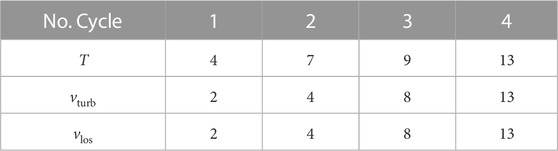
TABLE 1. Number of nodes at each cycle for the thermodynamics variables considered during the inversions.

2.2 Selected pointy profiles

The selection of the extremely pointy profiles and the very pointy profiles was made through visual inspection. Thanks to the clustering of the data, this task is easily doable: we look for these peculiar profiles in a set of 320 RPs instead of ≈ 8,000 profiles. We have selected the most clear cases of these profiles to show their main characteristics. We can distinguish two main groups among the extremely pointy profiles that we have classified as Type A and Type B (see Figures 3, 4). The core of the Mg II h&k extremely pointy profiles Type A (panel C) resembles the core of a Lorenztian distribution, while the wings look like the wings of a Laplacian distribution. The C II 1,334 & 1,335 Å lines are pointy, red-shifted, and in most cases their shape shows a negative skew (panel A). In some cases, the C II 1,334 & 1,335 Å lines saturate the response of the detector.

The Mg II h&k extremely pointy profiles type B (see panel C in Figure 4), in addition to having the pointy core, show very enhanced wings. Sometimes, the blue wing is slightly more enhanced than the red wing, making the k₃ and the h₃ features identifiable. The Mg II h&k lines are a bit shifted to the red. The Mg II UV triplet lines are clearly shifted to the red, and they have a blue component (panel B). Interestingly, the same happens for the C II 1,334 & 1,335 Å lines (panel A).

The last type of profile seems to be a combination of types A and B (see Figure 5). The main difference is the presence of a well-defined, stronger blue component, and the peak of the line is now well-centered. Note that the blue component is well distinguished, and the profile can be clearly described in terms of the 2v, 2r, and 3 features, that means, in terms of 2 peaks and the central depression. In this case, the 2r feature largely dominates over the 2v one, and it is located on the rest spectral position of the line. On the other hand, the 3 feature is present, and it is slightly blue-shifted. The wings of these profiles are not as enhanced as those of the extremely pointy profile of type B. As we will see in Section 4, the subtle differences between the profiles belonging to the combination type and the ones belonging to the type B are related to the slightly different stages of the flare’s evolution.

In all the types, the Mg II UV triplet lines show either a blue or red component, or both (see Figure 3). These components appear, in most cases, both in the Mg II UV1 line and the Mg II UV2&3 lines. This behavior indicates that these components are actually belonging to these lines and not to nearby lines in emission.

The spatial distribution of these profiles is shown in the right panel of Figure 1. The Type A profiles are mostly located in the ribbon (dark blue ticks), the type B profiles are located in the leading edge (dark orange ticks), and the combination type profiles are mostly located close to (and just trailing) the leading edge (dark green ticks). The locations displayed in light colors show all the profiles of the various types not shown in Figures 3–5. The profiles associated with these locations have a range of gradually changing appearances within their corresponding type. For instance, a profile in a light blue location is an extremely pointy type A profile but the wings of the Mg II h&k lines look more Lorentzian than Laplacian, in contrast to the most intense ones shown in Figure 3, which have more Laplacian wings.

The pointy profiles almost always occur in the flare ribbons. Pointy profiles have also been observed during the pre-flare phase, as we have already mentioned. However, it is during the maximum of the flare that the extreme and very pointy profiles appear.

2.3 Where in the solar atmosphere we can trust the model atmosphere associated to the pointy profiles

The main characteristic of the profiles studied in this paper is the pointy aspect in the core of the Mg II h&k lines, to some extent in the C II 1,334 & 1,335 Å lines, and a strong emission of the Mg II UV triplet lines. Another important feature of these profiles is the broad width of the lines, especially in their wings. This broadening affects all the lines mentioned above. Because the radiation of the wings comes from deeper in the atmosphere, we have investigated how deep in the model atmosphere the information recovered from the inversion is still reliable.

The traditional method to recover this information is by using the response function (RF, Mein, 1971; Landi Degl’Innocenti and Landi Degl’Innocenti, 1977) of the profile to a small variation of a physical parameter in the model atmosphere associated with the synthetic profile. In our case, this synthetic profile is the one that best fits the observation (inverted profile, in fuchsia line in all the figures of this paper). The background image of the panels in Figure 6 shows the normalized RF of the intensity (I) to changes in the temperature (panels A–C), v_los (D–F), and v_turb (G–I) for the extremely pointy inverted profile type shown in fuchsia in Figure 7. The observed and inverted profiles are shown as a reference for a better location in wavelength of the spectral features of the profile. In the RF background image, the stronger the color is the stronger the response of I at that wavelength is to a variation of the physical parameter at that optical depth. Note that the RFs are evaluated for each physical parameter independently.

In this paper, we have considered another approach: to determine at what optical depth the synthetic profile obtained from the modified model associated with the inverted profile deviates from that inverted profile. We have modified the T and the n_e by changing these values with the FALC model values, starting from log(τ) = 0 to log(τ) = −7 with steps of Δτ = 0.2. Similarly, we have changed the v_turb and the v_los to 0 km s⁻¹ in the same optical range. This method has the advantage that considers simultaneously the 4 physical parameters, while the RFs quantify the impact of the perturbation of only one physical variable in the profile.

In most of the cases analyzed, the inverted profile remains as it is, ignoring the modifications we have made to the atmosphere, up to log(τ) ≈ − 2.0, which means: any change in the model atmosphere at −2 ≲ log(τ) has no effect on the shape in the associated synthetic profile. Figure 8 shows the extremely pointy profile shown in Figure 7 in the dotted solid black line and the inverted profile in fuchsia in panels A to D, and the model atmosphere in solid colored lines in the last row of the figure in panels E and F. The profile in the dashed black line in panels A to D corresponds to the synthesis of the model shown in the last row in dashed black line as well. This modified model differs from the model atmosphere (in colors) associated to the inverted profile (in fuchsia) between $-2.2<\log (\tau )<0$, but it is just after $\log (\tau )\approx -2.0$ when the new synthetic profile (dashed black line) starts to be different with respect to the original inverted profile (in fuchsia). As we can see, the wings of the Mg II h&k lines obtained from the modified model atmosphere start to deviate from the inverted profile. This also happens in the extended wings of the Mg II UV triplet lines. We have to mention that this deviation occurs at log(τ) ≈ − 1.8 in other pointy profiles, such is the case for the profile shown in Figure 11. Any perturbation in the model at $\log (\tau )<-2.2$ produces a dramatic deviation from the inverted profile. Thus, those profiles showing extended, enhanced broad wings, either in the Mg II h&k lines or the Mg II UV triplet lines, are sensitive to the variations in the high-photosphere. This is also observed in the RFs shown in Figure 6, with the significant response at the extended wings of the Mg II h&k at $\log (\tau )<-2.2$ for T, v_los, and v_turb, while for the Mg II UV1 the response to variation of these parameters is still important at $\log (\tau )<-2.2$, but it is at as low as $\log (\tau )<-1.8$ for the v_los and at $\log (\tau )<-2.0$ for the v_turb. As a result, we should be cautious with the values of the model atmosphere between $-2.0<\log (\tau )<-1.8$, and completely discard the values for $-1.8<\log (\tau )<0$ shown in the figures of this paper. Because of this, the values in this optical depth range are gradually shaded in red.

FIGURE 8

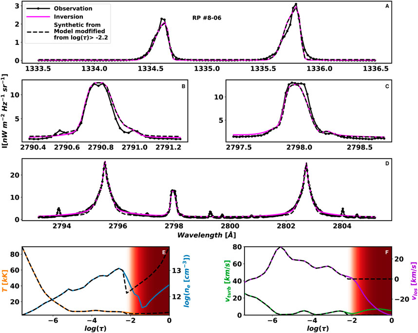
FIGURE 8. Deviation from the inverted profile corresponding to the extremely pointy type A profile (in fuchsia) shown in the Figure 7 that shows how sensitive the synthetic profile [dashed black line, panels from (A–D)] is along the solar atmosphere the model atmosphere [panels (E,F)]. The profile in dashed black line shows the resulting profile by considering a modified version [in dashed black lines, panels (E,F)] of the original model [in colors in the lower panels, panels (E,F)] from $-2.2<\log (\tau )<0$. See details in the main text.

To support this statement more strongly, we have verified that the photospheric lines available in the IRIS Mg II h&k spectral range do not show a high Doppler shift. We will use photospheric lines to recover the information from this optical depth range in a following investigation.

As it has been already mentioned, the values at log(τ)$<-6.5$ should be taken with caution. This is because the current inversion scheme is not able to capture changes in the thermodynamics - if any - in that optical depth range, i.e., well inside the transition region, from the C II 1,334 & 1,335 Å lines. None of the lines in this study are sensitive to changes in the thermodynamics at −1 < log(τ). Therefore, the values shown at these two ranges are due to the interpolation used by the inversion code in the nodes at that optical depths, and we have tested that changing those values in these ranges has no effect on the inverted profiles.

3 Results

Figures 7, 9, 10, 11 show the results from the inversions of two profiles of type A, one of type B, and a combination profile, respectively. These figures show the fit of the C II 1,334 & 1,335 Å lines, Mg II UV1 line, and the Mg II handk lines, including the Mg II UV2&3 blended lines. They show both the inversion considering only the latter lines and all together. Thus, we can better appreciate the impact in the model atmosphere by including the C II 1,334 & 1,335 Å lines and the Mg II UV1line. The physical parameters are shown along the logarithm of the optical depth, log(τ)⁴.

FIGURE 9

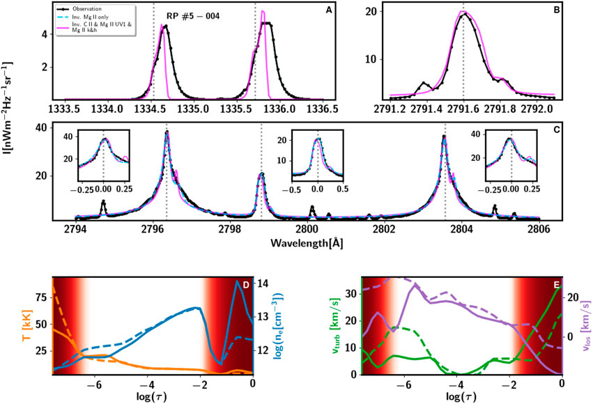
FIGURE 9. Inversion (fit) of the C II 1,334 & 1,335 Å, Mg II UV1  Mg II h&k, and Mg II UV2&3 lines of another extremely pointy profile type A, and the model recovered from the inversion. See caption of Figure 7 for details.

FIGURE 10

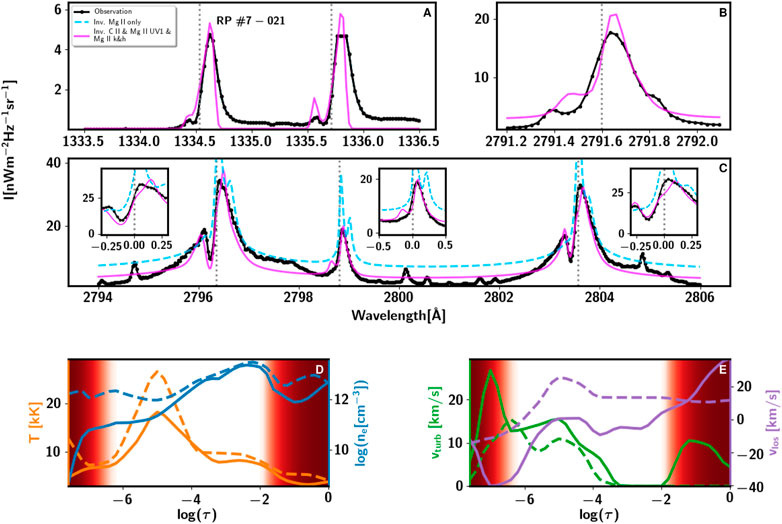
FIGURE 10. Inversion (fit) of the C II 1,334 & 1,335 Å, Mg II UV1  Mg II h&k, and Mg II UV2&3 lines of an extremely pointy profile type B, and the model recovered from the inversion. See caption of Figure 7 for details.

FIGURE 11

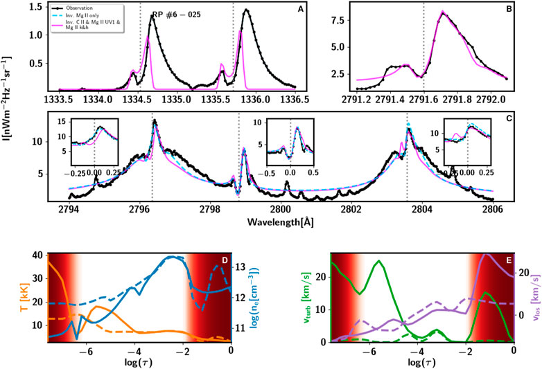
FIGURE 11. Inversion (fit) of the C II 1,334 & 1,335 Å, Mg II UV1  Mg II h&k, and Mg II UV2&3 lines of a combined pointy profile type, and the model recovered from the inversion. See caption of Figure 7 for details.

The model atmosphere obtained differs for the different types of pointy profiles. We first discuss the main behavior of the extremely pointy profiles A (Figures 7, 9), then the type B (Figure 10), and finally the combined type (Figure 11).

The fit of the spectral lines in Figure 7, while not perfect, is rather good in all the lines. In the high chromosphere⁵, the T shows large values, between 25 kK and 7.5 kK, as the optical depth increases. The n_e shows a steady, small increase around log (n_e) ≈ 12. The v_los goes from 0 km s⁻¹ to $\approx +30$ km s⁻¹, that is, a downflow with a strong gradient in the v_los. These values are very similar to the ones obtained in the inversion of the profiles shown in Figure 9. The v_turb  however, shows a difference. In the first case (Figure 7), the v_turb is close to 0 between −6 < log(τ)$<-5$, then increases up to 15–20 km s⁻¹ at log(τ) = −6.5. In the second case of pointy profile type A (Figure 9) the value is almost constant around v_turb= 5 km s⁻¹. Because the fit, especially the width of the lines, in the first case is good in all the lines - including the C II 1,334 & 1,335 Å an lines, we consider the v_turb$\approx 15-20$ km s⁻¹ as a valid value. In the second case, the fit of the C II 1,334 & 1,335 Å lines is not good, failing to fit the width of these lines. This, as it has been mentioned above, may be due to the dual optical behavior of these lines. Therefore, the values of v_turb must be considered carefully, especially in the higher part of the chromosphere, i.e., at $\log (\tau )<-6$. In the mid and low chromosphere, both cases behave very similarly: i) the and T decreases gradually, reaching its minimum value at log(τ) = 1, ii) the n_e increases up to log (n_e) = 13 at log(τ) = −2, then it drops off to 13 < log (n_e) < 12 at log(τ) = −1, iii) the v_los decreases gradually from 30 km s⁻¹ to 0 km s⁻¹, and iv) the v_turb shows a wavy behavior around 5 km s⁻¹.

The profiles in Figure 10 show an extremely pointy profile of type B. The T is lower in the high chromosphere ($\approx 10$ kK) than in the mid chromosphere ($\approx 15$ kK). The n_e in the high chromosphere has a lower value (log (n_e) ≈ 11) than for the pointy type A profiles. The T and n_e reach their minimum value at log(τ)= −1. The v_turb is $\approx 15$ km s⁻¹ in the high chromosphere, decreasing rapidly to 0 in the low chromosphere. The v_los shows a steep gradient in the upflow velocity at the high chromosphere, from −40 km s⁻¹ to 0 km s⁻¹, becoming and a downflow of $\approx +5$ km s⁻¹ in the low chromosphere.

The atmosphere corresponding to the combined type (Figure 11) is more similar to the one corresponding to type B than to type A. The most significant difference with respect to type B results are: i) the large value of the v_turb in the high chromosphere, with a value as high as 20–25 km s⁻¹, which explains by the very broad, enhanced wings, and ii) the smaller, more gradual upflow v_los varying from −10 km s⁻¹ to 0 km s⁻¹ from the high to the low chromosphere.

The fits of the C II 1334 & 1335 Å lines in 10, 11, and 12 are not good. To model and invert the C II 1334 & 1335 Å lines, especially in explosive events, is challenging. The fit of these lines is satisfactory in many cases, e.g., in active regions (Sainz Dalda et al., 2022), and even during pre-flare conditions (Woods et al., 2021). However, during the maximum of a flare, the physical conditions may be too complex to model and invert these lines properly with the currently available tools. As we mentioned above, these lines can be also formed in the transition region. Therefore, the inversion code must have the capability to reproduce the large jump in the temperature from the chromosphere to the transition region in very few optical depths. This is not possible with the current inversion scheme. As a consequence, the fit of the C II 1334 & 1335 Å lines in Figures 9, 10, 11 is not as satisfactory as in simpler conditions. A deeper investigation into the C atom model and an improved inversion code will likely help to fit these complex profiles, but this falls out of the scope of this paper.

3.1 How the extremely pointy profiles are formed

A simple way to create an extremely pointy type A profile in the Mg II h&k lines is by considering an extreme gradient in the high chromosphere. Figure 12 shows how to get an extremely pointy profile type A from a double-peaked Mg II h&k profile. The red and blue profiles are the result of considering the T, v_turb, and n_e of the double-peaked profile (panels D to F) with v_los shown in red and blue lines respectively (panel G) of Figure 12. In this example, the steep gradient is located between −7 < log(τ)$<-5.5$ and goes from ± 50 to 0 km s⁻¹. We have done several tests and we have also obtained extremely pointy profiles for lower values of v_los. Note that the C II 1,334 & 1,335 Å lines (panel A) are shifted to the red and blue wavelengths for the downflow and upflow gradients respectively, and they show the skewness previously observed in the IRIS data.

FIGURE 12

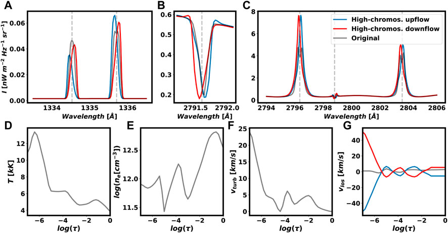
FIGURE 12. Creating an Mg II h&k extremely pointy profile type A [red or blue, in panels (A–C)] from a double-peaked Mg II h&k profile (grey) by considering an extreme gradient downflow (red) or upflow (blue) in the high chromosphere [panel (G)].

Another way of studying what can cause pointy profiles is by studying the contribution of v_los to the synthetic profile obtained by the inversion of the extremely pointy type A profile shown in Figure 7 (in fuchsia). We have taken the same thermodynamics atmosphere associated with that profile (see bottom panels in the 6) and imposed a zero velocity at all optical depths (v_los(τ) = 0 km s⁻¹), and then synthesized that new atmosphere. Again, we obtain a double-peaked profile (panels B and C), which is shown in blue in Figure 13.

FIGURE 13

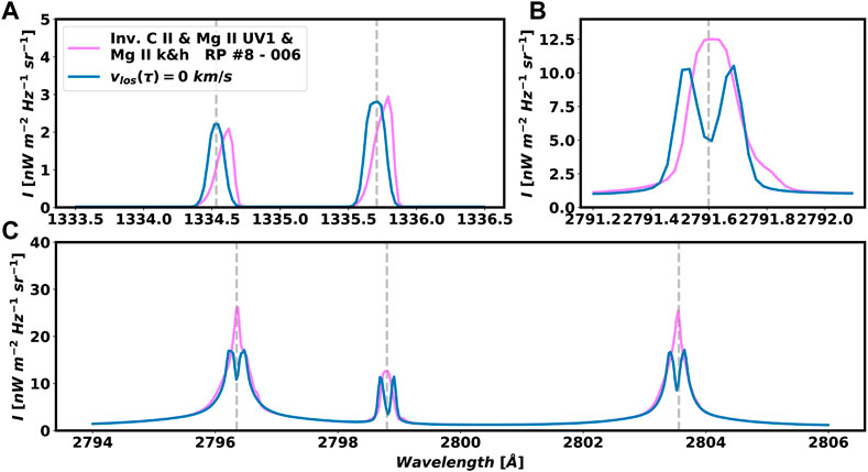
FIGURE 13. Deconstruction of the synthetic extremely pointy type A profile (in fuchsia) shown in the Figure 7 that shows the role played by the v_los. Panels A, B and C show the C II 1334 & 1335 Å, Mg II UV1, and the Mg II h&k lines (including Mg II UV2&3 lines) respectively. The profile in blues shows the resulting profile by considering v_los= 0 km s⁻¹ in the atmosphere associated to the profile mentioned above (two bottom panels in the Figure 7).

The role played by the v_los in the enhancement or diminution of emission peaks in the line was first studied by Scharmer (1984), and more recently by de la Cruz Rodríguez et al. (2015). Thus, a v_los to the blue (red) is able to reduce the line opacity in the red wing, and as a result an enhancement in the red (blue) wing of the line is produced. In addition, in the presence of a strong gradient of v_los  the core of the line (k₃) is shifted with respect to the wings, making it able to vanish one of the peaks of the line (k_2r or k_2v). Therefore, the enhancement of one of the peaks at the same time that the other peak is hidden by the shifted core produces an extremely pointy profile or a combined pointy profile.

In summary, the extremely pointy shape of these profiles is the signature of an extreme gradient in the v_los in the chromosphere. In the context of a flare, the downflows and upflows are associated with the chromospheric condensation and evaporation respectively. In this case, these flows have extreme gradients along the optical depth and take place in a well-determined optical depth range: the high chromosphere. Thus the difference between type A and type B is mainly due to the difference in the temperature in the high chromosphere, being smaller for the type B with respect to the type A.

4 Discussion

The inversion and interpretation of the profiles presented in this paper entail a significant challenge. The highly dynamic event studied - the maximum of an X1.0-class flare, is reflected both in the associated profiles and the thermodynamics recovered from the inversions of these profiles. The extremely pointy and combined type profiles belong to the same solar feature - the ribbon, including its leading and trailing edge. However, they are related to slightly different stages of the same event, which happen simultaneously in different locations in the ribbon. We should understand that both the variation in the appearance of the profiles and their associated thermodynamics is gradual. Thus, while we have focused our attention on the most significant of each type, the following interpretation captures the main physical properties during the maximum of the flare. Figure 14 is particularly helpful for this interpretation.

FIGURE 14

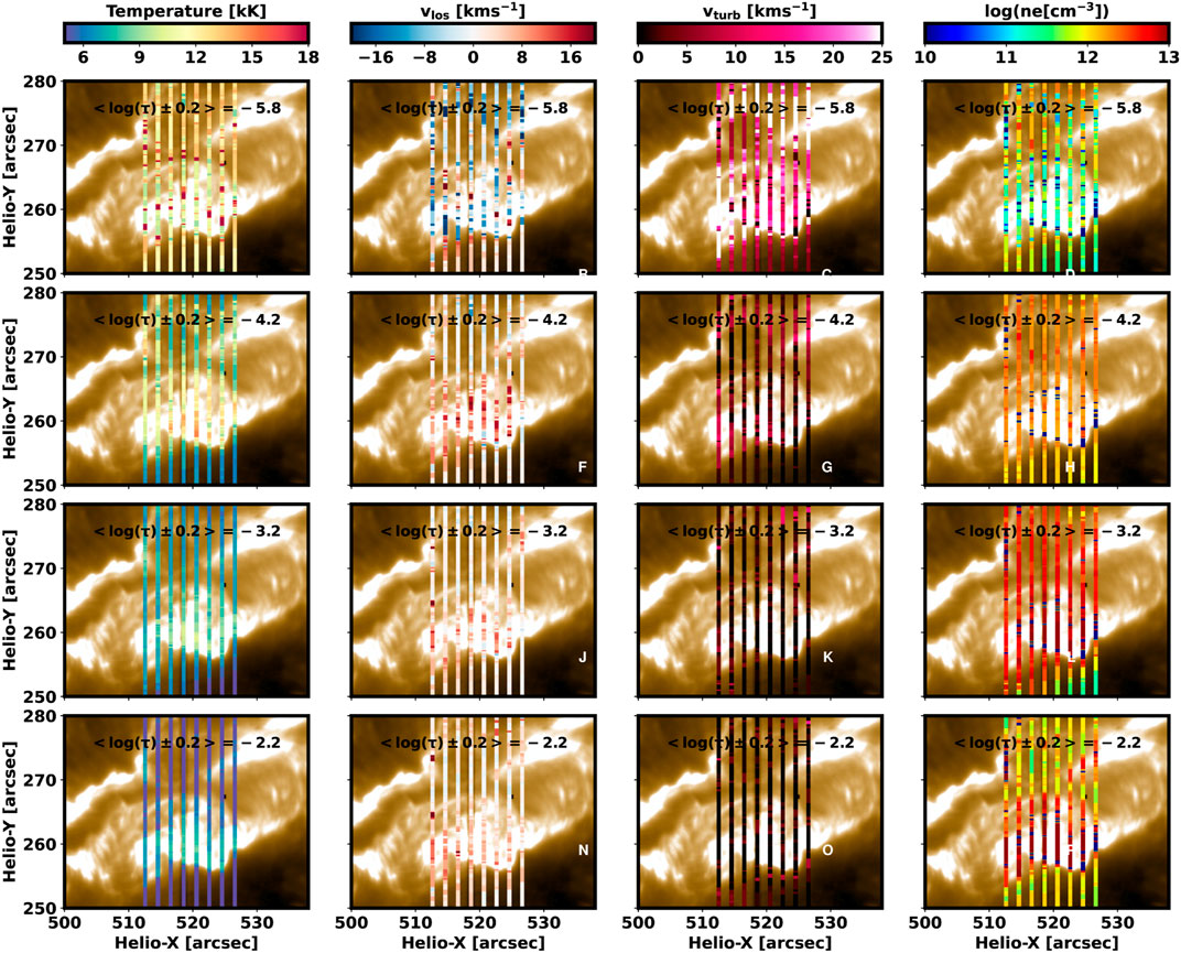
FIGURE 14. Maps of thermodynamic values (columns) during the maximum of the X1.0-class flare SOL2014-03-29T17:48, for various optical depths (rows). The image in the background of the panels corresponds to IRIS SJI 2796 Å shown in the dashed grey square in Figure 1.

For the positions scanned by the IRIS slit, the location of the trailing edge of the upper ribbon is at [X, Y] = [512, 268], and in the lower ribbon at [X, Y] = [517–526, 263]. It is in these locations where the extremely pointy type A profiles such as the ones shown in Figure 3 are found, while the rest of the profiles of this type are mostly located within the ribbon itself. The location for the leading edge of the upper ribbon is at [X, Y] = [512, 277] and in the lower ribbon at [X, Y] = [512–526, 257–255]. Most of the type B pointy profiles are located at the leading edge of the lower ribbon, while the combination profiles are located within the ribbon on the trailing side immediately adjacent to the leading edge and the ribbon of the ribbon (some are also located in the region just leading the trailing edge of the ribbon). Thus, as the ribbon is energized, starting from the trailing edge towards the leading edge, the profiles go from extremely pointy type A to the combination type and finally to type B.

Because ribbons propagate across the solar surface as the flare evolves, the spatial distribution of the thermodynamic parameters from trailing to leading edge of the ribbon provides a window into the typical temporal evolution within a single location. From the temporal evolution observed in the IRIS SJI data, we know that the trailing edge has been energized longer than the leading edge in the single snapshot shown in Figure 14. That could explain why in these locations the temperature is so high in the high chromosphere (log(τ) = −5.8, the first panel in the first row of Figure 14), while in the rest of the ribbon the high chromosphere temperature is lower. The trailing edge also differs from the rest of the ribbon when we consider the temperature difference between the high and middle chromosphere. In the trailing edge, the temperature of the high chromosphere is higher than in the mid chromosphere. In contrast, the mid chromosphere temperature (log(τ) = −4.2, the first panel of the second row of Figure 14) is higher than in the high chromosphere for the leading edge and interior of the ribbon itself. Thus, the bump in the temperature at log(τ) ≈ − 5 observed in Figure 10 has not reached yet the high-chromosphere, as it does in Figure 9 and even higher in Figure 7. This spatial pattern of a somewhat reduced temperature in the high chromosphere accompanied by an increase in the mid chromosphere is seen in both flare ribbons but most clearly in the lower ribbon as IRIS scanned this ribbon more fully. This pattern has been obtained in some numerical models of flare energy deposition in the chromosphere by Allred et al., 2015. These observations support a scenario in which energy is deposited in the middle chromosphere, with an associated increase in the local temperature. This energy deposition affects the high chromosphere at later times, as the flare evolves.

The most critical physical parameter that contributes to the very distinctive profiles studied in this paper is the line-of-sight velocity. As we have demonstrated, the extremely pointy profiles of the Mg II h&k lines, but also of the C II 1,334 & 1,335 Å lines, need the presence of a strong, divergent velocity gradient located between the high and middle chromosphere. Therefore, the main thermodynamic phenomenon in the chromosphere happening in the ribbons during the maximum of the flare is a divergent flow hosting strong velocity gradients.

In addition, the Mg II UV triplet lines have signatures associated with strong velocities in the high photosphere. The divergent flow located between the high and mid chromosphere can be appreciated between the first (i.e., top) and the second panel of the second column of Figure 14. There, we can observe predominantly an upflow in the ribbon in the high chromosphere (log(τ) = −5.8), while in the middle chromosphere and lower regions in the atmosphere (−4.2 < log(τ)) the ribbon shows a downflow. Note that in the trailing edge, there are some locations where the velocities in the high chromosphere are positive, i.e., they host downflows. Again, these locations are likely ahead in time (i.e., have evolved for the longest time since the start of the flare), so it is possible they may have experienced the upflows at an earlier stage of their evolution. The presence of a divergent flow is compatible with a scenario where an electron beam propagating downwards from the flare reconnection site in the corona impacts the dense chromosphere (thick-target model, Hudson and Ohki, 1972). Such divergent flows have also been obtained in radiation hydrodynamic experiments by Kerr et al., 2016 and Kowalski et al., 2017 who studied the same flare that we analyzed in the current paper. However, the synthetic Mg II h&k profiles obtained by Kerr et al., 2016 show the k₃ feature in absorption, which indicates that their models are missing some ingredient(s) needed to reproduce the observed profiles. Similarly, the temperature increase where the divergent flows occur in Kowalski et al., 2017 is much higher (T ≈ 10 MK) than the one we obtain. What can explain the strong velocity flows that we observe in the high photosphere? Several results suggest that these can be explained by the different penetration of the different energy regimes of the electron beams. Graham et al., 2020 demonstrated that low-energy electrons (E ≈ 25–50 keV) are responsible for the evaporation-condensation in the high chromosphere, while very high-energy electrons (E ≥ 50 keV) can penetrate deeper into the atmosphere and produce a similar situation in the high photosphere. These authors used, in addition to the Mg II UV1 line, the optically thin lines Fe I 2814.11 Å, and Fe II 2813.3 and 2814.45 Å. In their study all these lines show a strong red component. However, in the flare we study here no red components are present in the Fe I and Fe II lines, and the Mg II UV1 line shows on occasion a strong red component, but also blue and red components in other cases. Likely, the situation shown in Figure 14 is compatible with the scenario described by Graham et al., 2020 and the one previously suggested by Libbrecht et al., 2019 (see Figure 14 of their paper). Here, in agreement with Graham et al., 2020, we interpret that the bounce-back motion that Libbrecht et al., 2019 locates in the chromosphere is lower in our case, reaching the high photosphere. In summary, there are two slabs, one located between the high and mid chromosphere and the other in the high photosphere, that are suffering the impact from energized electron coming from the corona, and producing explosive, divergent upflows and downflows. These slabs are not necessarily located in the same feature of the ribbon at the same time, and their location evolves as the ribbon is energized by the flare.

Finally, in the ribbons the velocity associated turbulent motions is large, v_turb$\approx 10-20$km s⁻¹, in the high and mid chromosphere in the ribbons. It is in these regions where the core of both the C II 1,334 & 1,335 Å lines and the Mg II handk lines is sensitive to this parameter. The values presented in this investigation are more realistic than the ones obtained by Rubio da Costa and Kleint (2017) (40 km s⁻¹) or Zhu et al. (2019) (40–50 km s⁻¹). In the low chromosphere and the high photosphere the vturb in the ribbons is negligible. The extended, broad wings of the Mg II h&k are sensitive to changes in v_turb in the mid chromosphere, while the Mg II UV triplet lines are sensitive to turbulence in the low chromosphere. We also note that the electron density in the ribbons is 12 < log (n_e) < 13 in the chromosphere, reaches its maximum in the low chromosphere with a value of log (n_e) ≈ 15, just before the temperature minimum, which is pushed down (in terms of the optical depth) towards the low-photosphere (log(τ) ≈ − 1). Thus, the extended wings of the Mg II h&k lines are mostly due to the thermodynamics conditions in the chromosphere. This region is where the contribution function of these lines is prominent when a flare model F2 (Machado et al., 1980) and non-LTE are considered, as it is shown in Figure 16 of Liu et al. (2015). This authors found that the contribution to the winds of the Mg II h&k lines in a F2 flare model extends in a region of ≈ 1,000 km in the chromosphere, in comparison to a ≈ 200 km when the VALC quiet-sun model (Vernazza et al., 1981) is considered. However, because in their model the v_turb$\approx 0-10$ km s⁻¹, and it is uniform in the formation region of the Mg II h&k lines, the authors justify the large broadening of the observed wings to an enhanced line source function rather than an extra broadening. Our results prove that reasonable v_turb values varying along the optical depth are able to reproduce the width of the Mg II h&k lines.

The spectral profiles studied in this article are challenging to model and interpret due to the complexity of the physical conditions that generate them. In addition to belonging to an extreme event (an X1-class flare), we note that several physical processes such as upflows and downflows, or heating and cooling, occur simultaneously in the same structure—the ribbon. We are analyzing the maximum of the flare, but that does not mean all regions in the ribbon show the same behavior. For example, the trailing edge experiences different physical conditions than the ribbon itself. The interpretation of the peculiar profiles clearly will depend on where and when they are observed in the macroscopic spatiotemporal evolution of the flare. Until now there have not been any theoretical or numerical models that are able to properly reproduce these profiles. In this context, our investigation and results provide strict observational constraints to these models and suggest a reasonable physical scenario.

Data availability statement

Publicly available datasets were analyzed in this study. This data can be found to strictly the following text: https://www.lmsal.com/hek/hcr?cmd=view-event&event-id=ivo%3A%2F%2Fsot.lmsal.com%2FVOEvent%23VOEvent_IRIS_20140329_140938_3860258481_2014-03-29T14%3A09%3A382014-03-29T14%3A09%3A38.xml.

Author contributions

This paper has been led by ASD. He has made the analysis of the IRIS spectra, and the interpretation of the inversions and the models recovered from them, as well as the main contain of the manuscript. BDP has contributed with meaningful ideas, enlightening discussions with AD, and with critical comments and improvements to the manuscript. All authors contributed to the article and approved the submitted version.

Funding

ASD was supported in part by the NASA contract NNG09FA40C (IRIS) and the NASA grant 80NSSC21K0726 “Understanding the role played by the turbulence in the chromosphere during flares”. BDP was supported by NASA contract NNG09FA40C (IRIS).

Acknowledgments

IRIS is a NASA small explorer mission developed and operated by LMSAL with mission operations executed at NASA Ames Research Center and major contributions to downlink communications funded by ESA and the Norwegian Space Agency. The authors thank the helpful discussions and clarifications made by J. de la Cruz Rodríguez. We also thanks him for sharing the state-of-the-art inversion code STiC, which is available to the public.

Conflict of interest

The authors declare that the research was conducted in the absence of any commercial or financial relationships that could be construed as a potential conflict of interest.

Publisher’s note

All claims expressed in this article are solely those of the authors and do not necessarily represent those of their affiliated organizations, or those of the publisher, the editors and the reviewers. Any product that may be evaluated in this article, or claim that may be made by its manufacturer, is not guaranteed or endorsed by the publisher.

Footnotes

¹By shape of a profile or a line, we mean the spectral distribution of the intensity (specifically, the spectral radiance) with respect to the wavelength in a given spectral range.

²https://iris.lmsal.com/iris2/iris2_chapter01.html#limitations-of-iris2-inversions

³https://www.youtube.com/watch?v=55sT144u5ag

⁴In this paper, log actually means log₁₀, and log(τ) means log₁₀(τ₅₀₀), being τ₅₀₀ the reference of the optical depth unity corresponding to the continuum at 500 nm.

⁵Roughly speaking, in this paper, we refer to the high chromosphere as the optical depth range −6.5 < log(τ)$<-5$, the mid chromosphere is −5 < log(τ)$<-4$, the low chromosphere is −4 < log(τ)$<-2$, the high photosphere is −2 < log(τ)$<-1$, and the low photosphere is −1 < log(τ)$<0$. These ranges are dynamically changing, especially for events such as flares. Throughout such changes, the region just above the temperature minimum is referred to as the low chromosphere, while the steep, large increase of the temperature at small log(τ) values is the top of the chromosphere.

References

Allred, J. C., Kowalski, A. F., and Carlsson, M. (2015). A unified computational model for solar and stellar flares. Astrophysical J.809, 104. doi:10.1088/0004-637X/809/1/104

CrossRef Full Text | Google Scholar

Avrett, E. H., Machado, M. E., and Kurucz, R. L. (1986). “Chromospheric flare models,” in The lower atmosphere of solar flares Editors D. F. Neidig, and M. E. Machado (United States: National Solar Observatory), 216–281.

Google Scholar

Carlsson, M., Leenaarts, J., and De Pontieu, B. (2015). What do IRIS observations of Mg II k tell us about the solar plage chromosphere?Astrophysical J.809, L30. doi:10.1088/2041-8205/809/2/L30

CrossRef Full Text | Google Scholar

Carlsson, M., and Stein, R. F. (1995). Does a nonmagnetic solar chromosphere exist?Astrophysical J.440, L29. doi:10.1086/187753

CrossRef Full Text | Google Scholar

Carlsson, M., and Stein, R. F. (1997). formation of solar calcium H and K bright grains. Astrophysical J.481, 500–514. doi:10.1086/304-043

CrossRef Full Text | Google Scholar

de la Cruz Rodríguez, J., Hansteen, V., Bellot-Rubio, L., and Ortiz, A. (2015). Emergence of granular-sized magnetic bubbles through the solar atmosphere. II. Non-LTE chromospheric diagnostics and inversions. Astrophysical J.810, 145. doi:10.1088/0004-637X/810/2/145

CrossRef Full Text | Google Scholar

de la Cruz Rodríguez, J., Leenaarts, J., and Asensio Ramos, A. (2016). Non-LTE inversions of the Mg II h & k and UV triplet lines. Astrophysical J.830, L30. doi:10.3847/2041-8205/830/2/L30

CrossRef Full Text | Google Scholar

de la Cruz Rodríguez, J., Leenaarts, J., Danilovic, S., and Uitenbroek, H. (2019). STiC: A multiatom non-LTE PRD inversion code for full-Stokes solar observations. A&A623, A74. doi:10.1051/0004-6361/201834464

CrossRef Full Text | Google Scholar

De Pontieu, B., Title, A. M., Lemen, J. R., Kushner, G. D., Akin, D. J., Allard, B., et al. (2014). The Interface region imaging Spectrograph (IRIS). Sol. Phys.289, 2733–2779. doi:10.1007/s11207-014-0485-y

CrossRef Full Text | Google Scholar

del Pino Alemán, T., Casini, R., and Manso Sainz, R. (2016). Magnetic diagnostics of the solar chromosphere with the Mg II h-k lines. Astrophysical J.830, L24. doi:10.3847/2041-8205/830/2/L24

CrossRef Full Text | Google Scholar

Dimitrijević, M. S., and Sahal-Bréchot, S. (1998). Electron-impact broadening of MgII spectral lines for astrophysical and laboratory plasma research. Phys. Scr.58, 61–71. doi:10.1088/0031-8949/58/1/009

CrossRef Full Text | Google Scholar

Dimitrijević, M. S., and Sahal-Bréchot, S. (1995). Stark broadening parameter tables for Mg II. Bull. Astron. Belgr.151, 101–114.

Google Scholar

Feldman, U., and Doschek, G. A. (1977). The 3s-3p and 3p-3d lines of Mg II observed above the solar limb from Skylab. Astrophysical J.212, L147. doi:10.1086/182395

CrossRef Full Text | Google Scholar

Graham, D. R., Cauzzi, G., Zangrilli, L., Kowalski, A., Simões, P., and Allred, J. (2020). Spectral signatures of chromospheric condensation in a major solar flare. Astrophysical J.895, 6. doi:10.3847/1538-4357/ab88ad

CrossRef Full Text | Google Scholar

Hawley, S. L., and Fisher, G. H. (1994). Solar flare model atmospheres. Astrophysical J.426, 387. doi:10.1086/174075

CrossRef Full Text | Google Scholar

Hudson, H. S., and Ohki, K. (1972). Soft X-ray and microwave observations of hot regions in solar flares. Sol. Phys.23, 155–168. doi:10.1007/BF00153899

CrossRef Full Text | Google Scholar

Jefferies, J. T. (1968). Spectral line formation. A Blaisdell Book Pure Appl. Sci.1968.

Google Scholar

Kaiser, M. L., Kucera, T. A., Davila, J. M., Cyr, St.O. C., Guhathakurta, M., and Christian, E. (2008). The STEREO mission: An introduction. Space Sci. Rev.136, 5–16. doi:10.1007/s11214-007-9277-0

CrossRef Full Text | Google Scholar

Kerr, G. S., Allred, J. C., and Carlsson, M. (2019a). Modeling Mg II during solar flares. I. Partial frequency redistribution, opacity, and coronal irradiation. ApJ883, 57. doi:10.3847/1538-4357/ab3c24

CrossRef Full Text | Google Scholar

Kerr, G. S., Carlsson, M., and Allred, J. C. (2019b). Modeling Mg II during solar flares. II. Nonequilibrium effects. Astrophysical J.885, 119. doi:10.3847/1538-4357/ab48ea

CrossRef Full Text | Google Scholar

Kerr, G. S., Fletcher, L., Russell, A. J. B., and Allred, J. C. (2016). Simulations of the Mg II k and Ca II 8542 lines from an AlfvÉn wave-heated flare chromosphere. Astrophysical J.827, 101. doi:10.3847/0004-637X/827/2/101

CrossRef Full Text | Google Scholar

Kerr, G. S., Simões, P. J. A., Qiu, J., and Fletcher, L. (2015). IRIS observations of the Mg ii h and k lines during a solar flare. A&A582, A50. doi:10.1051/0004-6361/201526128

CrossRef Full Text | Google Scholar

Kleint, L., Battaglia, M., Reardon, K., Sainz Dalda, A., Young, P. R., and Krucker, S. (2015). The fast filament eruption leading to the X-flare on 2014 march 29. Astrophysical J.806, 9. doi:10.1088/0004-637X/806/1/9

CrossRef Full Text | Google Scholar

Kneer, F., Scharmer, G., Mattig, W., Wyller, A., Artzner, G., Lemaire, P., et al. (1981). OSO-8 observations of CAII H and K MGII H and K lyman-alpha and lyman-beta above a sunspot. Sol. Phys.69, 289–300. doi:10.1007/BF00149995

CrossRef Full Text | Google Scholar

Kohl, J. L., and Parkinson, W. H. (1976). The Mg II h and k lines. I. Absolute center and limb measurements of the solar profiles. Astrophysical J.205, 599–611. doi:10.1086/154317

CrossRef Full Text | Google Scholar

Kosugi, T., Matsuzaki, K., Sakao, T., Shimizu, T., Sone, Y., Tachikawa, S., et al. (2007). The Hinode (solar-B) mission: An overview. Sol. Phys.243, 3–17. doi:10.1007/s11207-007-9014-6

CrossRef Full Text | Google Scholar

Kowalski, A. F., Allred, J. C., Uitenbroek, H., Tremblay, P.-E., Brown, S., Carlsson, M., et al. (2017). Hydrogen balmer line broadening in solar and stellar flares. Astrophysical J.837, 125. doi:10.3847/1538-4357/aa603e

CrossRef Full Text | Google Scholar

Landi Degl’Innocenti, E., and Landi Degl’Innocenti, M. (1977). Response function for magnetic lines. A&A56, 111–115.

Google Scholar

Leenaarts, J., Pereira, T. M. D., Carlsson, M., Uitenbroek, H., and De Pontieu, B. (2013a). The Formation of iris diagnostics. I. A quintessential model atom of Mg II and general formation properties of the Mg II h&k lines. Astrophysical J.772, 89. doi:10.1088/0004-637X/772/2/89

CrossRef Full Text | Google Scholar

Leenaarts, J., Pereira, T. M. D., Carlsson, M., Uitenbroek, H., and De Pontieu, B. (2013b). The Formation of IRIS diagnostics. II. The formation of the Mg II h&k lines in the solar atmosphere. Astrophysical J.772, 90. doi:10.1088/0004-637X/772/2/90

CrossRef Full Text | Google Scholar

Lemaire, P., Choucq-Bruston, M., and Vial, J. C. (1984). Simultaneous H and K Ca ii, h and k Mg ii, Lα and Lβ H i profiles of the April 15, 1978 solar flare observed with the OSO-8/L.P.S.P. experiment. Sol. Phys.90, 63–82. doi:10.1007/BF00153785

CrossRef Full Text | Google Scholar

Lemaire, P., and Gouttebroze, P. (1983). Magnesium II line formation - the contribution of high atomic levels to the resonance lines. A&A125, 241–245.

Google Scholar

Lemaire, P., and Skumanich, A. (1973). Magnesium II doublet profiles of chromospheric inhomogeneities at the center of the solar disk. A&A22, 61.

Google Scholar

Libbrecht, T., de la Cruz Rodríguez, J., Danilovic, S., Leenaarts, J., and Pazira, H. (2019). Chromospheric condensations and magnetic field in a C3.6-class flare studied via He I D₃ spectro-polarimetry. A&A621, A35. doi:10.1051/0004-6361/201833610

CrossRef Full Text | Google Scholar

Lin, R. P., Dennis, B. R., Hurford, G. J., Smith, D. M., Zehnder, A., Harvey, P. R., et al. (2002). The reuven ramaty high-energy solar spectroscopic imager (RHESSI). Sol. Phys.210, 3–32. doi:10.1023/A:1022428818870

CrossRef Full Text | Google Scholar

Lites, B. W., and Cook, J. W. (1979). A semiempirical model of the upper flare chromosphere. Astrophysical J.228, 598–609. doi:10.1086/156884

CrossRef Full Text | Google Scholar

Lites, B. W., and Skumanich, A. (1982). A model of a sunspot chromosphere based on OSO 8 observations. Astrophysical J.49, 293–315. doi:10.1086/190800

CrossRef Full Text | Google Scholar

Liu, W., Heinzel, P., Kleint, L., and Kašparová, J. (2015). Mg II lines observed during the X-class flare on 29 march 2014 by the Interface region imaging Spectrograph. Sol. Phys.290, 3525–3543. doi:10.1007/s11207-015-0814-9

CrossRef Full Text | Google Scholar

Machado, M. E., Avrett, E. H., Vernazza, J. E., and Noyes, R. W. (1980). Semiempirical models of chromospheric flare regions. Astrophysical J.242, 336–351. doi:10.1086/158467

CrossRef Full Text | Google Scholar

MacQueen, J. (1967). “Some methods for classification and analysis of multivariate observations,” in Proc. Of the fifth berkeley symposium on mathematical statistics and probability Editors L. M. Le Cam, and J. Neyman (California: University of California Press), 281–297.

Google Scholar

Manso Sainz, R., del Pino Alemán, T., Casini, R., and McIntosh, S. (2019). Spectropolarimetry of the solar Mg II h and k lines. Astrophysical J.883, L30. doi:10.3847/2041-8213/ab412c

CrossRef Full Text | Google Scholar

Mein, P. (1971). Inhomogeneities in the solar atmosphere from the Ca II infra-red lines. Sol. Phys.20, 3–18. doi:10.1007/BF00146089

CrossRef Full Text | Google Scholar

Panos, B., Kleint, L., Huwyler, C., Krucker, S., Melchior, M., Ullmann, D., et al. (2018). Identifying typical Mg II flare spectra using machine learning. Astrophysical J.861, 62. doi:10.3847/1538-4357/aac779

CrossRef Full Text | Google Scholar

Panos, B., Kleint, L., and Voloshynovskiy, S. (2021). Exploring mutual information between IRIS spectral lines. I. Correlations between spectral lines during solar flares and within the quiet sun. Astrophysical J.912, 121. doi:10.3847/1538-4357/abf11b

CrossRef Full Text | Google Scholar

Pereira, T. M. D., Carlsson, M., De Pontieu, B., and Hansteen, V. (2015). The Formation of IRIS diagnostics. IV. The Mg II triplet lines as a new diagnostic for lower chromospheric heating. Astrophysical J.806, 14. doi:10.1088/0004-637X/806/1/14

CrossRef Full Text | Google Scholar

Pereira, T. M. D., Leenaarts, J., De Pontieu, B., Carlsson, M., and Uitenbroek, H. (2013). The Formation of IRIS diagnostics. III. Near-Ultraviolet spectra and images. Astrophysical J.778, 143. doi:10.1088/0004-637X/778/2/143

CrossRef Full Text | Google Scholar

Pereira, T. M. D., and Uitenbroek, H. (2015). RH 1.5D: A massively parallel code for multi-level radiative transfer with partial frequency redistribution and zeeman polarisation. A&A574, A3. doi:10.1051/0004-6361/201424785

CrossRef Full Text | Google Scholar

Pesnell, W. D., Thompson, B. J., and Chamberlin, P. C. (2012). The solar dynamics observatory (SDO). Sol. Phys.275, 3–15. doi:10.1007/s11207-011-9841-3

CrossRef Full Text | Google Scholar

Rathore, B., Carlsson, M., Leenaarts, J., and De Pontieu, B. (2015). The Formation of IRIS diagnostics. VI. The diagnostic potential of the C II lines at 133.5 nm in the solar atmosphere. Astrophysical J.811, 81. doi:10.1088/0004-637X/811/2/81

CrossRef Full Text | Google Scholar

Rathore, B., and Carlsson, M. (2015). The Formation of iris diagnostics. V. A quintessential model atom of C II and general formation properties of the C II lines at 133.5 nm. Astrophysical J.811, 80. doi:10.1088/0004-637X/811/2/80

CrossRef Full Text | Google Scholar

Rubio da Costa, F., and Kleint, L. (2017). A parameter study for modeling Mg II h and k emission during solar flares. Astrophysical J.842, 82. doi:10.3847/1538-4357/aa6eaf

CrossRef Full Text | Google Scholar

Rubio da Costa, F., Kleint, L., Petrosian, V., Liu, W., and Allred, J. C. (2016). Data-driven radiative hydrodynamic modeling of the 2014 march 29 X1.0 solar flare. Astrophysical J.827, 38. doi:10.3847/0004-637X/827/1/38

CrossRef Full Text | Google Scholar

Sainz Dalda, A., Agrawal, A., De Pontieu, B., and Gosic, M. (2022). IRIS²⁺: A comprehensive database of stratified thermodynamic models in the low solar atmosphere. arXiv e-prints , arXiv:2211.

Google Scholar

Sainz Dalda, A., de la Cruz Rodríguez, J., De Pontieu, B., and Gošić, M. (2019). Recovering thermodynamics from spectral profiles observed by iris: A machine and deep learning approach. Astrophysical J.875, L18. doi:10.3847/2041-8213/ab15d9

CrossRef Full Text | Google Scholar

Sánchez Almeida, J., and Lites, B. W. (2000). Physical properties of the solar magnetic photosphere under the MISMA hypothesis. II. Network and internetwork fields at the disk center. Astrophysical J.532, 1215–1229. doi:10.1086/308603

CrossRef Full Text | Google Scholar

Scharmer, G. B. (1984). “Accurate solutions to non-LTE problems using approximate Lambda operators,” in Methods in radiative transfer (Cambridge: Cambridge University Press), 173–210.

Google Scholar

Steinhaus, H. (1957). Sur la division des corps matériels en parties. Bull. Acad. Pol. Sci.4, 801.

Google Scholar

Sukhorukov, A. V., and Leenaarts, J. (2017). Partial redistribution in 3D non-LTE radiative transfer in solar-atmosphere models. A&A597, A46. doi:10.1051/0004-6361/201629086

CrossRef Full Text | Google Scholar

Thorndike, R. L. (1953). Who belongs in the family?Psychometrika18, 267–276. doi:10.1007/BF02289263

CrossRef Full Text | Google Scholar

Uitenbroek, H. (2001). Multilevel radiative transfer with partial frequency redistribution. Astrophysical J.557, 389–398. doi:10.1086/321659

CrossRef Full Text | Google Scholar

Uitenbroek, H. (1997). THE solar Mg II h and k lines - observations and radiative transfer modeling. Sol. Phys.172, 109–116. doi:10.1023/A:1004981412889

CrossRef Full Text | Google Scholar

Vernazza, J. E., Avrett, E. H., and Loeser, R. (1981). Structure of the solar chromosphere. III. Models of the EUV brightness components of the quiet sun. Astrophysical J.45, 635–725. doi:10.1086/190731

CrossRef Full Text | Google Scholar

Woods, M. M., Sainz Dalda, A., and De Pontieu, B. (2021). Unsupervised machine learning for the identification of preflare spectroscopic signatures. Astrophysical J.922, 137. doi:10.3847/1538-4357/ac2667

CrossRef Full Text | Google Scholar

Xu, Y., Cao, W., Ding, M., Kleint, L., Su, J., Liu, C., et al. (2016). Ultra-narrow negative flare front observed in helium-10830 Å using the 1.6 m new solar telescope. ApJ819, 89. doi:10.3847/0004-637X/819/2/89

CrossRef Full Text | Google Scholar

Zhu, Y., Kowalski, A. F., Tian, H., Uitenbroek, H., Carlsson, M., and Allred, J. C. (2019). Modeling Mg II h, k and triplet lines at solar flare ribbons. Astrophysical J.879, 19. doi:10.3847/1538-4357/ab2238

CrossRef Full Text | Google Scholar