A comparative study of data-driven MHD simulations of solar coronal evolution with photospheric flows derived from two different approaches

1 Introduction

The environment of the upper atmosphere of the Sun, i.e., the solar corona, is dominated by the magnetic field and often experiences impulsive eruption events, most of which have originated from solar active regions (ARs). The magnetic field that is concentrated in the ARs stores adequate energy for solar eruptions (Chen, 2011) by coupling the variations in the lower and higher atmospheres together. However, since we cannot effectively measure the 3D magnetic field in the solar corona heretofore, static modeling such as the non-linear force-free field (NLFFF) extrapolation from the photospheric magnetograms is often used to estimate the coronal magnetic fields (Sun et al., 2012; Jiang and Feng, 2013; Okuzumi et al., 2016; Duan et al., 2019; Wiegelmann and Sakurai, 2021). Though NLFFF is a physically reasonable approximation (Lüst and Schlüter, 1954; Chandrasekhar and Woltjer, 1958), it is only valid for the quasi-steady state of the solar corona, which however is frequently interrupted by eruptions. To model the evolution of real ARs, we have to implement the dynamic models, in particular, the magnetohydrodynamics (MHD) simulation, with the bottom boundary conditions matching the observables on the photosphere in a time-dependent way.

At the photosphere, as driven by the solar dynamo and near-surface convections, sunspots (and magnetic flux tubes in all different scales) evolve continuously with highly complicated motions (e.g., emergence and cancellation of magnetic flux as well as shearing and converging motions), all of which are difficult to mimic in artificial settings. Therefore, the idea of data-driven modeling was implemented in a full MHD model for the first time by Wu et al. (2006) to obtain the evolutionary state of the target AR. With the development of observations and numerical methods, different data-driven models have been proposed and can be classified into three types according to the different realizations of the driving boundary conditions (see a review on this topic by Jiang et al., 2022), i.e., the B-driven model (Wu et al., 2009; Mackay et al., 2011; Jiang et al., 2016a; Jiang et al., 2016b) where the magnetograms are input at the bottom boundary directly; the E-driven model (Cheung and DeRosa, 2012; Cheung et al., 2015; Hayashi et al., 2018; Pomoell et al., 2019; Price et al., 2019; Inoue et al., 2022; Chen et al., 2023; Inoue et al., 2023) where the magnetic field at the bottom boundary is driven by the pre-determined photospheric electric field; and the V-driven model (Guo et al., 2019; Hayashi et al., 2019; Liu et al., 2019; He et al., 2020; Jiang et al., 2021a; Zhong et al., 2021) where with the photospheric velocity fields derived first, the magnetic field at the bottom boundary evolves according to the magnetic induction equation.

Though the B-driven method seems to be a straightforward option since the magnetogram can be fully matched, it introduces magnetic divergence errors from the bottom boundary, which often require extra methods to deal with (Tóth, 2000). If we use the vector potential A to implement the data-driven method, there will be no extra divergence error. However, deriving the vector potential at the photosphere may require the help of the “poloidal–toroidal decomposition” (PTD), as in the PDFI method described below, which may not be an easy task and will further increase the complexity of the B-driven method. In the E-driven model, the shortage of introducing the divergence error vanishes automatically because after taking the divergence of the magnetic induction equation, the time-changing rate of the magnetic divergence is zero, therefore the magnetic divergence will not change as the MHD system evolves. The main difficulty of implementing the E-driven method arises from inversion of the photospheric electric fields, which includes both the inductive and non-inductive parts. Great progress has been made in solving this problem (Fisher et al., 2010; Fisher et al., 2012; Kazachenko et al., 2014; Fisher et al., 2015), as shown by benchmark tests. These contributions finally converged into the PDFI_SS software (Fisher et al., 2020). We note that even in the E-driven model, the photospheric flow has to be properly set to follow the Ohm’s law, and solving the complex momentum equation will cost numerical resources a lot. Therefore, if the velocity field on the photosphere can be pre-determined, the momentum equation will not have to be solved at the bottom boundary and the electric field will not appear in model equations, both of which are convenient for implementing the data-driven simulation, which is the outstanding advantage of the V-driven model when compared to the others.

Since direct observation of the photospheric flow is often absent, a variety of methods have been proposed for deriving the photospheric flow from magnetograms. Among them, the most famous is the local correlation tracking (LCT) method (November and Simon, 1988; Chae, 2001), in which the transverse motion of the magnetic flux element is captured according to an advection equation, i.e., ∂_tB_z = −u_LCT ⋅∇B_z. Thus, only the velocity tangential to the photosphere is derived, and moreover, it does not represent the actual plasma velocity strictly (Démoulin and Berger, 2003) since the LCT method does not obey the magnetic induction equation. For improving the capability of the LCT-type technique, several variants of the LCT method have also been proposed (Kusano et al., 2002; Kusano et al., 2004; Welsch et al., 2004; Fisher and Welsch, 2008), and some of them can obtain the full three components of the photospheric flow. Different from the LCT method, Schuck (2006) uses the variational principle to minimize the bias of the magnetic induction equation to estimate the photospheric flow from observed magnetograms, named the differential affine velocity estimator (DAVE) method. The more frequently used is the updated version of DAVE, i.e., the differential affine velocity estimator for vector magnetograms (DAVE4VM) method (Schuck, 2008), which has been applied recently for V-driven simulation. For example, Hayashi et al. (2019) used the projected normal characteristic (PNC) method to update the bottom magnetic field using the DAVE4VM velocity. In their model, the magnetic energy could not be injected into the solar corona efficiently; however, using the DAVE4VM velocity, this problem was resolved by Jiang et al. (2021b) by solving the magnetic induction equation directly instead of using the PNC method. The remaining problem in their results was that there was a magnetic flux pileup at the edge of their target AR, which made the photospheric magnetic field generated in their model different from the observation. Though in some data-driven models (Guo et al., 2019; Liu et al., 2019; He et al., 2020; Zhong et al., 2021), the magnetic field was made to fully match the observations by simultaneously inputting both the magnetic and velocity fields at the bottom boundary, the magnetic induction equation still might not be satisfied at the bottom boundary. To overcome all these shortcomings, our ultimate goal is to develop a V-driven model that can generate almost the same evolution of the magnetic field in simulation with vector magnetograms under the constraint of the magnetic induction equation.

To go one step further toward this target, in this article, we test the performance of the widely used DAVE4VM and advanced PDFI methods [the acronym ‘PDFI’ stands for “PTD plus Doppler plus Fourier local correlation tracking (FLCT) plus Ideal” contributions to the electric field], both of which are used to generate the photospheric flow field, in our DARE-MHD model (Jiang et al., 2016a; Jiang et al., 2021a; Wang et al., 2022; Wang et al., 2023). The DAVE4VM and PDFI velocities were input at the bottom boundary to drive the AR NOAA 11158 to evolve from 14 February 2011 00:00 UT to 15 February 2011 00:00 UT. This AR is remarkably active and produces an X2.2 class flare around 01:44 UT on 15 February, and has been widely studied (Jing et al., 2012; Sun et al., 2012; Wang et al., 2012). For example, Lumme et al. (2019) compared the DAVE4VM and PDFI methods by calculating the magnetic energy and helicity directly from observation in different cadences, showing a similar behavior before the flare onset. This AR in the studied period was located close to the solar disk center and thus provided high-quantity data. To mimic the enhanced photospheric diffusion in our simulation, we set the magnetic diffusion η decrease as the local scale of the magnetic field increase. With this empirical setting, the simulation results derived by the PDFI velocity perform better in the evolution of the total magnetic energy and total unsigned magnetic flux. It also has a more reasonable consistency with observations of AIA 131 Å. On the contrary, the morphology of the sunspots generated by the DAVE4VM velocity is more similar to observations, as characterized by the correlation coefficient for the observed magnetogram and simulation results.

The remainder of this article is organized as follows. First, we describe the basics of AR 11158 and the model we used in Section 2. In Section 3, we compare the simulation results by different velocity fields and finally give our discussion and conclusion in Section 4.

2 Observation and model

2.1 Observation

AR 11158 was constituted of two bipolar regions that emerged before 15 February 2011, forming a complex quadrupole topology. The opposite magnetic polarities near the main polarity inversion line (PIL) collided and sheared with each other (can be seen in the 24-h evolution as shown in Figures 1A, B), injecting the magnetic energy continuously during their emergence stage, which may have finally contributed to the onset of the X2.2 flare (accompanied by a halo CME) around 01:44 UT on 15 February. At that time, this AR was located at S21W21, which was not far from the solar disk center (Figure 1C) (Schrijver et al., 2011).

FIGURE 1

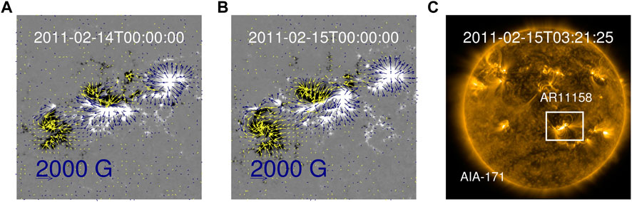
FIGURE 1. (A) Yellow(blue) vectors denote the transverse magnetic field on the photosphere, where B_z < 0 (B_z > 0) on 14 February 2011 at 00:00 UT, and the black and white of the background represent the negative and positive magnetic flux, respectively. (B) Same as A, but on 15 February 2011 at 00:00 UT. (C). A full-disk image of AIA 171 Å, with AR 11158 in the white rectangle.

2.2 Model

To study the energy accumulation process before the flare onset, we employ the DARE-MHD model, which solves the full 3D MHD equations, with the non-dimensionalized form given by

$\begin{array}{cc}\hfill \frac{\partial \rho }{\partial t}+\nabla \cdot \left(\rho \mathbf{v}\right)& =-{\nu }_{\rho }\left(\rho -{\rho }_0\right)\hfill \\ \hfill \rho \frac{D\mathbf{v}}{Dt}& =-\nabla p+\mathbf{J}\times \mathbf{B}+\rho \mathbf{g}+\nabla \cdot \left(\nu \rho \nabla \mathbf{v}\right)\hfill \\ \hfill \frac{\partial \mathbf{B}}{\partial t}& =\nabla \times \left(\mathbf{v}\times \mathbf{B}-\eta \mathbf{J}\right)\hfill \\ \hfill \frac{\partial T}{\partial t}+\nabla \cdot \left(T\mathbf{v}\right)& =\left(2-\gamma \right)T\nabla \cdot \mathbf{v}\hfill \end{array}(1)$

where J = ∇ ×B, g is the solar gravity, and γ = 1 is the adiabatic index. By setting ν_ρ = 0.05 V_A, where V_A is the Alfvén velocity, the plasma density will relax to its initial value ρ₀ within a timescale of 20 Alfvén time τ_A, which can avoid extremely low densities, thus making the magnitude of the time step to an acceptable level for efficient iteration. The kinetic viscosity ν is given as ν = 0.05 Δx/Δt, with Δx (varying from 0.5 arcsecs to 8 arcsecs in our simulation) and Δt being the spatial resolution and time step, respectively, to maintain the numerical stability. We used no explicit magnetic resistivity in our simulation to mimic the highly conductive plasma in the hot solar corona. In an eruption event, a strong shock travels to the lateral and top boundaries. Therefore, the computational domain is usually set to be sufficiently large to prevent the initial mechanism of eruptions from being affected by improper lateral/top boundary conditions. In this work, we do not intend to reproduce the eruption in AR 11158, and thus we set the simulation box relatively small to [−184, 184] Mm in the x, y directions and [0, 368] Mm in the z direction, with the side and top boundary conditions as described in Section 2.2.2. The Powell source term[−(∇ ⋅B) v] and the diffusion control term[∇(μ∇ ⋅B)] are added to the right-hand side of the magnetic induction equation to deal with the magnetic divergence error, as described by Jiang et al. (2010). Here, μ is a spatially varying parameter that was properly chosen to maximize the diffusion without introducing numerical instability.

2.2.1 Initial conditions

We initialize the magnetic field in our simulation using the magnetograms in the Coronal Global Evolutionary Model (CGEM) data series, which include the longitudinal, latitudinal, and radial components of the photospheric magnetic field (Schou et al., 2012), Doppler velocity (Welsch et al., 2013), and the line-of-sight (LOS) unit vector, respectively. To reduce the measurement errors, the original magnetic field was smoothed using Gaussian smoothing with FWHM (the ‘full width at half maximum’ of the Gaussian function used in smoothing) of 6 arcsecs. Then, an NLFFF was extrapolated from the smoothed CGEM magnetogram on 14 February 2011 at 00:00 UT using the CESE-MHD-NLFFF code (Jiang and Feng, 2013), in which a set of zero-β MHD equations were solved to seek an approximately force-free equilibrium. We reduced the magnitude of the extrapolated field by a factor of 25 for saving the computational time. The initial plasma background was set as an isothermal model with a uniform temperature of the typical value of T = 1 × 10⁶ K in the solar corona. Therefore, to mimic the realistic corona background with the reduced NLFFF, we modified the solar gravity (Jiang et al., 2021b) to make the minimum plasma β as 8 × 10⁻⁴ and maximum Alfvén speed V_A ∼ 5,357 km s⁻¹ in the initial equilibrium that we obtain below. Finally, we input the NLFFF to the modified plasma background with a zero bottom velocity until the MHD system relaxed to the equilibrium state, i.e., the kinetic and magnetic energy kept almost unchanged, and the initial state was ready.

2.2.2 Boundary conditions

At the bottom boundary, we energized the system using two types of photospheric velocity (as independently derived by either DAVE4VM or PDFI) by solving the non-ideal magnetic induction equation $\frac{\partial \mathbf{B}}{\partial t}=\nabla \times (\mathbf{v}\times \mathbf{B})+\eta {\nabla }_{\perp }^2\mathbf{B}$ using the finite difference method, where ${\nabla }_{\perp }^2=\frac{{\partial }^2}{{\partial }^2{x}^2}+\frac{{\partial }^2}{{\partial }^2{y}^2}$ is the surface Laplace’s operator (Aulanier et al., 2009). The derivation of DAVE4VM velocity v_D is straightforward, using three components of the original magnetic field with a window size of 19 (Liu and Schuck, 2012). For PDFI velocity, we first derived the electric field E_P using the PDFI_SS software and then calculated the PDFI velocity as ${\mathbf{v}}_{\mathrm{P}}=\frac{{\mathbf{E}}_{\mathrm{P}}\times \mathbf{B}}{B^2}$. The two velocity fields were smoothed using Gaussian smoothing with a FWHM of 6 arcsecs to reduce unexpected errors. As an example, Figure 2C shows the horizontal velocity and Figure 2D shows the vertical velocity at the time 14 February 2011 00:00 UT as calculated by the two different methods, both of which give rather different results. Specifically, the PDFI velocity is often parallel with, while the DAVE4VM one is perpendicular to, the edge of the AR (labeled as “edge” in Figure 2), which could be explained intuitively as follows. Near the edge of sunspots, there exists the famous “moat” flow (Sheeley, 1972; Brickhouse and Labonte, 1988) that can be traced by the motion of the magnetic flux, and the DAVE4VM method solves the vertical component of the magnetic induction equation $\frac{\partial B_z}{\partial t}=\nabla \cdot (v_z{\mathbf{B}}_{\mathbf{t}}-B_z{\mathbf{v}}_{\mathbf{t}})$ in the least-square sense. Therefore, the DAVE4VM velocity is highly influenced by the motion of the moat flow, which is nearly perpendicular to the edge of the sunspots. However, the motion of the magnetic flux may not represent the plasma flow. In the PDFI method, the full induction equation is solved directly, the solution of which will be closer to the actual flow of photospheric material. Furthermore, the velocity field corresponding to the non-inductive electric field is also obtained. As shown in Figures 2A, B, it is the velocity corresponding to the non-inductive part that mainly contributes to the PDFI velocity perpendicular to the sunspot’s edge, thus it is not surprising that the superposition of both will behave differently from the DAVE4VM velocity there. In addition, we note that this may be the reason why there was the magnetic flux concentrating at the edge of the sunspots as seen in our previous simulations as driven by the DAVE4VM velocity. Near the main PIL, both methods lead to shearing flow (labeled as ‘PIL’ in Figure 2), which can inject free energy efficiently. Two vertical velocity fields are also distributed differently, as shown in Figures 2E, F, and we show the average velocity field obtained by two methods in Figure 3. Before being input at the bottom surface, two velocity fields were strengthened by a factor of 13.7 (determined by $\frac{720\mathrm{s}\mathrm{e}\mathrm{c}\mathrm{o}\mathrm{n}\mathrm{d}}{0.5\times 105\mathrm{s}\mathrm{e}\mathrm{c}\mathrm{o}\mathrm{n}\mathrm{d}}$, where 720 is the time cadence of original magnetograms and 0.5 × 105 is the time cadence for inputting the bottom flow in simulation), and thus the timescale of our simulation is shortened by the same times. In addition to the velocity and magnetic field on the photosphere, we also added magnetic diffusion at the bottom boundary to mimic the photospheric diffusion effect originating from the granular and supergranular convection (Wang et al., 1989), as well as small-scale turbulent diffusion that is relevant to the scale length. Therefore, we set the photospheric η empirically as

$\eta =\min \left(0.1,\left[\exp \left(5\times 10^{-4}{L}^{-5}\right)-1\right]\times 2\times 10^{-3}\right)(2)$

with $L=\frac{B}{\sqrt{\Vert \nabla B{\Vert }_2}}$ being the local scale length of the magnetic field. This ensures a larger η in the region where the small-scale magnetic field appeared, which effectively dispersed the magnetic flux pileup on the photosphere as shown in our previous studies (Jiang et al., 2021a; Wang et al., 2023) but not seen in observations. On the side and top boundaries, we choose to extrapolate all the eight MHD variables from the neighboring inner points with zero normal gradients of the boundary surface to mimic the open boundary, except the normal component of the magnetic field is updated by the divergence-free condition to reduce the divergence errors.

FIGURE 2

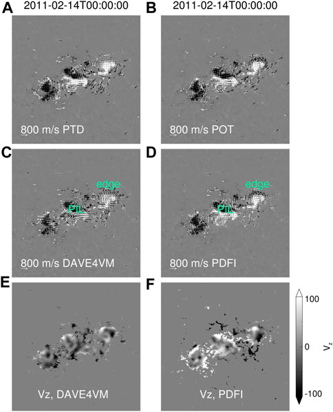
FIGURE 2. (A) Vectors denote the transverse velocity field derived by the PTD method on 14 February 2011 at 00:00 UT, and the background is the same as described in Figure 1A. (B–D) Same as A, but denotes the contributions of the non-inductive electric field of the PDFI method, and the transverse velocity field derived by the DAVE4VM and PDFI methods, respectively. The green ‘PIL’ and ‘edge’ labels indicate the regions where the two velocity fields differ from each other. (E) The distribution of the vertical DAVE4VM velocity. (F) The distribution of the vertical PDFI velocity. In six panels, the value of the velocity at the region where B_z < 100 G is set to be zero.

FIGURE 3

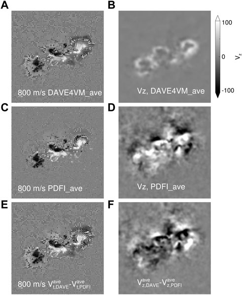
FIGURE 3. (A) Vectors denote the time average transverse velocity field derived by the DAVE4VM method from 14 February 2011 at 00:00 UT to 15 February at 00:00 UT. The background is the same as described in Figure 1A. (B) The time average vertical DAVE4VM velocity is from the same period as in A. (C) Same as A, but derived by the PDFI method. (D) Same as B, but derived by the PDFI method. (E) The direct difference of (A,C). (F) The difference between (B,D).

3 Results

The diffusion term on the bottom boundary plays an important role in our simulation. To understand its effect, first, we show the simulation results generated without the extra bottom diffusion as given in Section 2.2.2, and the results generated with the bottom extra diffusion are shown subsequently for comparison.

3.1 Results without extra diffusion

The evolution of magnetic and kinetic energies in DAVE4VM(PDFI) simulation are shown in Figures 4A, B. In both panels, the ideal magnetic energy injection (which means the electric field was derived according to the ideal Ohm’s law) that was calculated from observation [the black solid curve, which is calculated by the ideal Poynting flux at the bottom boundary using the DAVE4VM(PDFI) velocity and the observed magnetic field] deviates a little from the ideal magnetic energy injection in the simulation [the red solid curve, calculated by the ideal Poynting flux at the bottom boundary using the DAVE4VM(PDFI) velocity and the simulated magnetic field]. This deviation mainly arises from that the grid resolution is not high enough to capture the spatial variation of the magnetic field near the bottom surface, and this might be the same reason why the red curves deviate from the blue curves (the total magnetic energy, calculated by the volume integral of the magnetic energy density), for since when we used a higher grid resolution, the deviation will be smaller. The deviations between the red and blue curves are overall small, for which the total energy is approximately conserved in our simulation.

FIGURE 4

FIGURE 4. (A) Evolution curves of different energies in the DAVE4VM simulation. The black and red solid curves denote the magnetic energy injection calculated from observed magnetogram and simulation results, respectively, by integrating the ideal Poynting flux on the photosphere, i.e., ∫_photosphere(−V_D × B)×B ⋅ dS, where V_D is the DAVE4VM velocity. The blue and green solid curves denote the total magnetic and kinetic energy in the simulation, respectively. All the energy evolution curves are normalized by the magnetic energy of the potential field of the initial magnetogram E_p0 = 1.06 × 10³⁰ erg (a fixed value only used for normalization). When scaling to the realistic value, this value should be multiplied by a factor of 625 = 25², thus being 6.64 × 10³² erg. (B) Same as A, but obtained from the results driven by the PDFI velocity. (C) The black, blue, and green solid curves denote the total unsigned magnetic flux on the photosphere obtained by observed magnetogram, PDFI, and DAVE4VM simulation data, respectively, all of which have been normalized by their initial values. The dashed lines denote the flux canceled by extra bottom diffusion. Since we did not use the extra bottom diffusion, all curves in all three panels end at the early stage, representing the real-time duration of 2–3 h as the timescale has been shortened by a factor of 13.7 in simulations.

Since we did not use the extra diffusion, as shown by the blue (the total unsigned magnetic flux on the bottom boundary in the PDFI simulation) and black (the total unsigned magnetic flux of the magnetogram) solid curves in Figure 4C, the PDFI velocity had injected more magnetic flux than the observation, which suggests that the PDFI velocity overestimates the vertical component of the photospheric velocity. In addition, the PDFI velocity in the vertical direction (v_z) is larger than 0 in most areas as shown in Figures 3B, D. As a result, the DAVE4VM velocity injected less magnetic flux (the green solid curve in Figure 4C). To show the effect of bottom diffusion, we plot the blue and green dashed curves to represent the flux canceled by the extra bottom diffusion, which is computed by the direct difference between the magnetic flux in the simulation with (the blue and green solid curves in Figure 7C) or without (the blue and green solid curves in Figure 4C) the extra bottom diffusion.

From Figures 4A, B, it is obvious that without the extra bottom diffusion, both the DAVE4VM and PDFI run will fail after 10 minutes. The reason for the failure of both simulations comes from the bottom boundary, as shown in the last panel of Figures 5A, B. The white arrows indicate some small polarities, which are not seen in the observed magnetograms and are thus unphysical. They are the consequence of numerical instabilities that have resulted from the velocity-driven boundary conditions. Due to these unphysical polarities, the correlations between the simulation results and observations decrease fast (Figure 6) before the breakdown of the PDFI simulation (and at the end of the DAVE4VM simulation, the correlation of the B_x component also decreases). However, after using the extra bottom diffusion, these small polarities disappear, and the magnetic energy injection and total unsigned magnetic flux matched well with observations at the same time, all of which illustrate the positive effect of the extra diffusion, as discussed below.

FIGURE 5

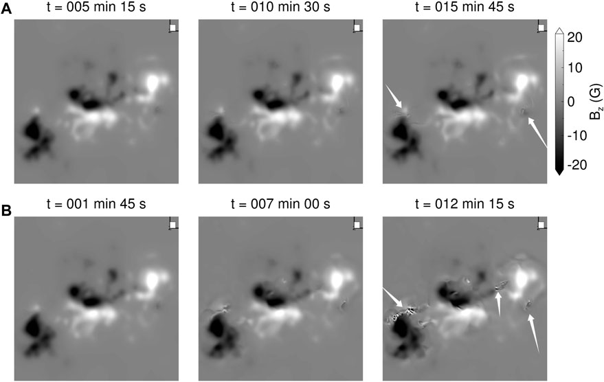
FIGURE 5. (A) Sunspots generated by the DAVE4VM velocity without extra bottom diffusion. The white arrows indicate some unphysical small polarities. (B) Same as A, but generated by the PDFI velocity.

FIGURE 6

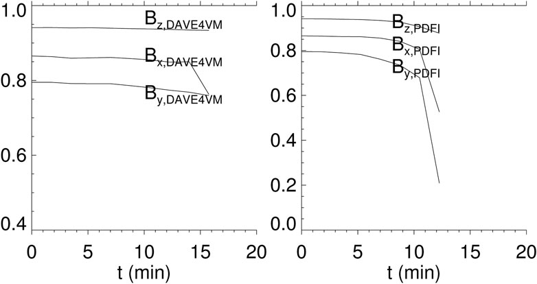
FIGURE 6. Curves in the left (right) panel denote the evolution of correlation coefficients for different components of the smoothed photospheric magnetic field from observations and the DAVE4VM (PDFI) simulation without extra bottom diffusion.

3.2 Results with extra diffusion

The evolution curves of different energies in the simulation using the DAVE4VM velocity are shown in Figure 7A, and the results for the PDFI velocity are shown in Figure 7B. It can be seen that with this extra bottom diffusion, both simulations perform well and do not break. The magnetic energy injection calculated from observation (the black solid curve) deviates from the magnetic energy injection in the simulation (the red solid curve) obviously. Though they are not the actual energy injection (since to calculate the Poynting flux, we assume the ideal Ohm’s law holds without considering the photospheric diffusion), this obvious deviation illustrates that the simulated magnetic field as driven by the DAVE4VM velocity should be much weaker than observations. An even worse result is that the total magnetic energy (the blue solid curve) decreases, which does not likely happen during this flux emergence stage. Such a large inconsistency is also seen in Figure 7C, i.e., the total unsigned flux (the green solid line) decreases, which is the opposite of the actual situation (the black solid line). However, these obtained quantitative features were much better in the simulation driven by the PDFI velocity. As shown in Figure 7B, the magnetic energy injection in the simulation matches very well with that of the observation, while again the deviation between the surface energy injection (the red solid curve) and the volume integrated energy (the blue solid curve) denotes the effect of surface diffusion. The deviation between energy injection and increase in both simulations can be understood in two ways: first, the enhanced photospheric diffusion will take effect at the bottom boundary, leading to the dispersion and cancellation of magnetic flux and therefore a reduction of the total magnetic energy. Second, with such a strong photospheric diffusion, the line-tied condition at the bottom boundary will be destroyed. As a result, the footpoints will slip and not move according to the photospheric velocity field (Jiang et al., 2021b), thus the actual energy injection will be lower than the ideal value (red curves in Figures 7A, B), which also manifests as a mismatch between the energy injection and energy increase. During the whole process of two simulations, the kinetic energy remains at a very low value of 10⁻³E_p0 (where E_p0 is the magnetic energy of the potential field of the initial magnetogram), which is an indication of quasi-static evolution. The good performance of the simulation with PDFI velocity is clearly shown in reproducing the total unsigned magnetic flux, of which the evolution curves from the simulation (blue solid line) and observation (black solid line) are almost identical. For instance, both curves exhibit two plateau stages at almost the same moments of t = 20 min and t = 80 min, and both curves end at a value of approximately 1.2. Since the form of η shown in Section 2.2.2 has been tuned and optimized for PDFI velocity, we have also adjusted the form of η for better performance of DAVE4VM velocity. However, if the η is high, the magnetic energy cannot be injected efficiently (Figure 7A); if we set a relatively low photospheric diffusion, there will be numerical instability on the bottom boundary. In conclusion, the DAVE4VM method did not perform well in these quantitative aspects during this period of the target AR in our model.

FIGURE 7

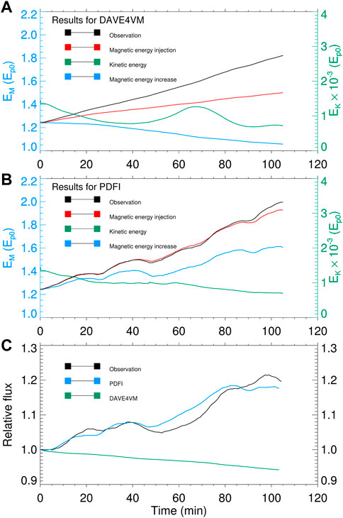
FIGURE 7. (A–C) All the settings are the same as in Figure 4, except the results are generated by the simulation with extra bottom diffusion, and there are no dashed lines in panel (C). All curves in all three panels end at t = 105.1 min, representing the real-time duration of 24 h as the timescale has been shortened by a factor of 13.7 in simulations.

Among the different states during the evolution of the magnetic field, the potential field has the minimum magnetic energy under the same boundary conditions. Therefore, the magnetic free energy, which provides the energy required in an eruption, always stores in the non-potential part, i.e., the current structure in the solar corona, which is shown in Figure 8. The current at t = 0 is labeled by the white arrow in Figure 8A, which is a whole piece and has a small volume, and then it transforms into quite distinct structures in different runs. In Figure 8B, it grows up but remains as a whole, while it divides into “1” and “2” in Figure 8C. The separating current layer in the PDFI simulation has a more reasonable consistency with observation in AIA 131 Å (visually has two discrete bright loops), and the synthetic image of coronal emission in the PDFI run (the last column in Figure 8B) also has two main brightening regions. The value of emission is constant along a field line and is assigned by the summation of the corona current density along the same field line traced from the bottom boundary. Then, we integrate the emission along the z direction to get the 2D total emission image. In addition to the coronal emission, we draw the field lines at the position of the two bright loops. In Figures 8G, H, labeled as “1” and “2,” there exist two groups of twisted field lines. Group “1” has a similar shape in Figures 8G, H, while group “2” behaves somewhat differently: having a smaller tilt angle with respect to the main PIL in the PDFI result, which is more consistent with the AIA-131 observation (Figure 8D). Though both results did not reproduce the observation very precisely, they clearly suggest a better performance of the PDFI method in our simulation of the coronal configuration.

FIGURE 8

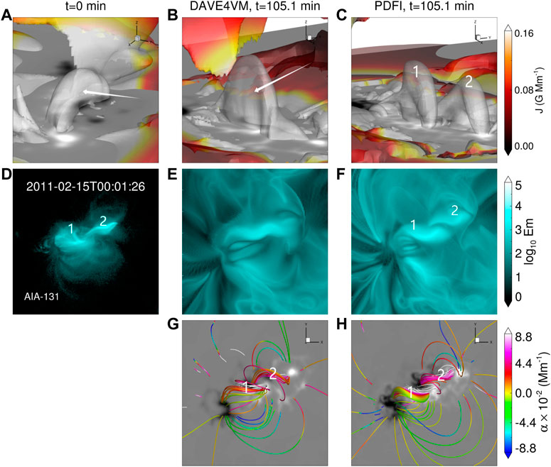
FIGURE 8. (A–C) Isosurface of J/B = 8.7 × 10⁻² Mm⁻¹, and the white arrows indicate the current layer near the main PIL. The initial current is shown in (A). The current at the end of the DAVE4VM and PDFI simulations is shown in (B,C), respectively. (D) The image of AIA 131 Å. (E) The synthetic image of coronal emission from the current density at the end of the DAVE4VM run. (F) Same as E, but at the end of the PDFI run. (G) The magnetic field lines at the end of the DAVE4VM run. (H) Same as G, but at the end of the PDFI run.

Since both simulations do not reproduce the observed magnetic field at the bottom surface, we are interested in how the simulation results of the two methods differ in spatial distribution from the observed magnetograms. We compare the results at the end of the two simulations with the observations made on 15 February 2011 at 00:00 UT in Figure 9, from which we can see the positive effect of the extra bottom diffusion that there will not be small unphysical magnetic polarities at the bottom boundary. Though we have used a rather large diffusion at the bottom surface, the DAVE4VM result (the third column of Figure 9C) still has some magnetic flux pileup at the edge of the AR (Jiang et al., 2021a), which is not seen in the PDFI result (Figure 9D). However, by a visual inspection of the flux distributions, we find that the DAVE4VM result is overall more similar observations than the PDFI one—a situation contrary to the results of comparison for the coronal configuration. The PDFI result appears to be more “turbulent,” especially for the horizontal components (B_x and B_y), while the DAVE4VM result is more smooth without the small-scale structures as shown in the PDFI result. To quantify the differences between the simulations and observations, we show the absolute value of the direct difference and correlation coefficients between our results and the smoothed magnetograms in Figures 10,11. In the DAVE4VM run, high photospheric diffusion weakened the magnetic field, leading to a lower magnetic energy injection rate. Thus, the main difference between simulation and observation may arise from the weaker magnitude of simulation results since the correlation coefficients are slightly higher than the PDFI ones (Figure 11). Whereas in the PDFI run, the difference mainly comes from the deviation of the location of the concentration of the magnetic flux, as indicated by the lower correlation coefficients. Comparing the constantly decreasing correlation coefficient curves, different components behave somewhat differently. The B_z,DAVE4VM and B_z,PDFI curves are higher than 0.85 all the time, showing a strong correlation between the simulation and observations. The B_x component performs a little poorly, while the B_y component is even worse and differs a lot in the two simulations. In Figure 11, the B_y,DAVE4VM curve is always higher than 0.7; however, the minimum value of the B_y,PDFI curve is close to 0.6, which is obviously lower than the others. This is consistent with the B_y column in Figure 9D, as the distribution of B_y is more dispersed than the observation. As a result, we conclude that the DAVE4VM velocity has a generally better capability in deriving the morphology of sunspots in our simulation. In addition, it is worth noting that for B_z, the initial value of correlation is very close to 1, while for B_x,y, it is just around 0.9. This reduction mainly arises from the construction of the initial state. As described in Section 2.2.1, the NLFFF was input into the DARE-MHD model to evolve to the initial equilibrium state, during which the bottom velocity was set to be zero. However, since we used the finite difference method to update the bottom magnetic field according to the magnetic induction equation, the non-zero velocity at the adjacent grid leads to the non-zero derivative, which will also change the bottom magnetic field and lead to the reduction of correlations.

FIGURE 9

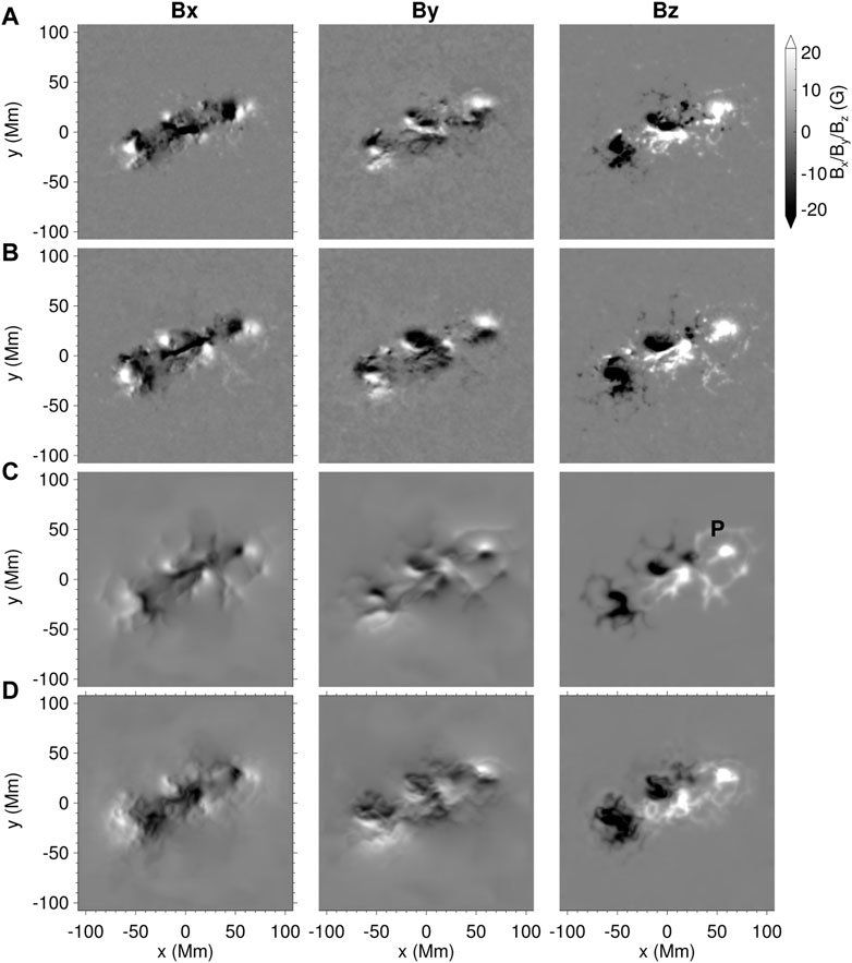
FIGURE 9. (A) Distribution of different magnetic field components of the smoothed vector magnetogram at 00:00 UT on 14 February 2011. (B) Same as A, but at 00:00 UT on 15 February. (C) The distribution of three magnetic field components on the bottom surface at the end of the DAVE4VM simulation. (D) Same as (C), but at the end of the PDFI simulation.

FIGURE 10

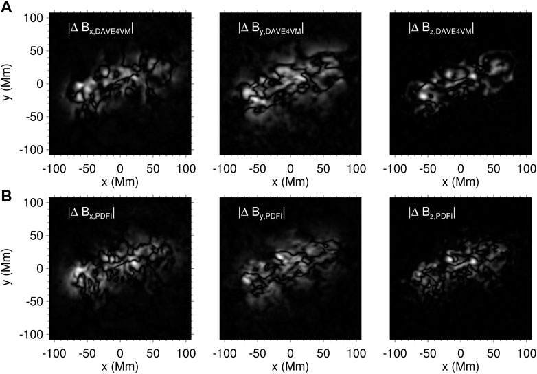
FIGURE 10. (A) Distributions of |ΔB_c,DAVE4VM| (c = x, y, and z), which is the absolute value of the direct difference between the bottom magnetic field of the DAVE4VM simulation and the smoothed magnetogram. (B) Same as A, but shows the distribution of |ΔB_c,PDFI|.

FIGURE 11

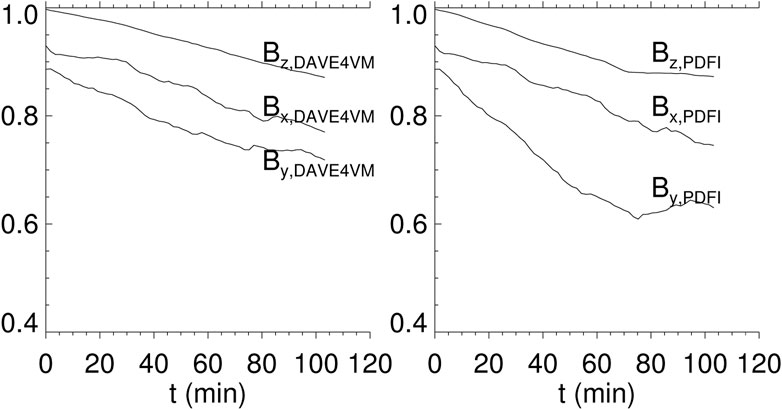
FIGURE 11. Curves in the left (right) panel denote the evolution of correlation coefficients for different components of the smoothed photospheric magnetic field from observation and the DAVE4VM (PDFI) simulation with extra bottom diffusion.

4 Conclusion and discussion

In this article, we have tested our DARE-MHD model for simulating the quasi-static evolution of AR 11158 on 14 February 2011 using two different velocity fields, which are calculated by the DAVE4VM and PDFI codes, respectively. The simulations are initialized with an MHD equilibrium obtained by relaxing the NLFFF extrapolated from the vector magnetogram of the starting time. To mimic the photospheric diffusion effect (which is larger than that in the solar corona), we used an enhanced surface diffusion term η depending on the local scale of the magnetic field. With this empirical setting, two series of photospheric flows derived from the time series of the magnetograms were applied to the bottom boundary to drive the initial equilibrium to evolve, and the bottom magnetic field was generated self-consistently by solving the magnetic induction equation on the bottom surface. The results of these two simulations have reasonable consistency with the observations in different aspects and also large differences between each other.

In the simulation driven by PDFI velocity, the magnetic energy injection and total unsigned magnetic flux matched well with those derived from magnetograms. However, they deviated substantially from the observations in the DAVE4VM run, especially the total magnetic energy and unsigned magnetic flux decreased, which may not happen during this flux emergence stage. The synthetic image of coronal emission in the PDFI run is also more similar to the AIA 131 Å observation than it is to the DAVE4VM run. The only discrepancy of the PDFI method in our simulation is the ability to reproduce the photospheric fields of the sunspots, as the DAVE4VM run performs better while the PDFI run results in structures that are a little dispersed and less (but not too much) correlated with the observations (as shown in Figure 11, only the curve of y component is obviously lower in the PDFI simulation). Nevertheless, since the target AR 11158 is close to the solar disk center and thus the data quality is high, great consistency between the PDFI results and observations demonstrates the superiority of the PDFI method in reproducing the magnetic energy injection, total magnetic flux, and the current structure, as well as the superiority of the DAVE4VM method in reproducing the correlations between the simulated photospheric magnetic field and the observed one in the V-driven model in this case study. The main unobserved feature driven by the DAVE4VM velocity, i.e., the flux pileup near the edge of the sunspots, nearly disappears in the PDFI simulation.

Since we used the enhanced bottom diffusion in both DAVE4VM and PDFI simulations, one may doubt whether the PDFI velocity can remove the flux pileup only with the extra bottom diffusion. It is difficult to test this idea using simulation directly because without the extra diffusion, both simulations can only be carried out for a short time duration. However, we can estimate this idea by inference, and the answer may be “no.” As we have discussed in Section 2.2.2, since the DAVE4VM method only solves the magnetic induction equation in the vertical direction, the DAVE4VM velocity will be strongly affected by the “moat”-flow-like motion, which can be observed by tracing the apparent motion of the magnetic flux elements. As a consequence, the DAVE4VM velocity will follow the trajectory of these flux elements, which may not be the actual photospheric flow. The PDFI method solves the full magnetic induction equation and will not be affected by the evolution of B_z so strongly. Therefore, the PDFI velocity does not have to be “moat”-flow-like near the sunspots’ edges (Figure 2A). Furthermore, it is the velocity field corresponding to the non-inductive electric field that mainly contributes to the flow that is parallel with the sunspots’ edges (Figure 2B), which can be explained as follows. Since the non-inductive electric field is the gradient of a scalar field, its curl vanishes, for which the non-inductive electric field will not contribute to the evolution of the bottom magnetic field, i.e., the velocity field corresponding to the non-inductive part should be along the contour of the magnetic field. These are the intrinsic reasons why PDFI velocity can remove the flux pileup at the edge of active regions.

Even with these improvements, there is still a large gap between the current models and the ultimate goal of developing the V-driven method that can reproduce the observed photospheric magnetic field. The reasons can be various. In the aspect of observation, there are inevitable errors in both the measurement of the magnetic field and Doppler velocity. It is also possible that the time cadence of measurement could not be sufficiently high in capturing the dynamics of the photosphere magnetic field, which might fundamentally lead to the inconsistency between simulation and observation. The other reason could originate from the FLCT method used in the PDFI_SS software because the FLCT method may not represent the actual plasma flow (Démoulin and Berger, 2003) and may result in a biased potential electric field. Improvements can possibly be made by replacing the FLCT technique with other more reliable methods. In addition, numerical models also have to be developed. In the solar corona, the magnetic field is often assumed to be force-free. However, during the early stage in flux emergence simulations, the photosphere may also have a strong Lorentz force and torque (Jiang and Toriumi, 2020) that need not be force-free. Therefore, other forces (e.g., gravity, pressure-gradient) by which the residual of the Lorentz force should be balanced also have to be specified by modeling the lower atmosphere, i.e., the photosphere, chromosphere, and transition region. With these advances, the dynamic process in the photosphere and chromosphere has the potential to be recreated in simulation more realistically, which may be helpful in reproducing the homologous eruption in data-driven models and even the whole life span of ARs.

Data availability statement

The original contributions presented in the study are included in the article/supplementary material; further inquiries can be directed to the corresponding author.

Author contributions

XW accomplished the simulation, performed the result analysis, and wrote the draft. CJ revised the text and images of the manuscript. All authors contributed to the article and approved the submitted version.

Funding

The work is jointly supported by the National Natural Science Foundation of China (Grant Nos. 42030204, 42174200), the National Key R&D Program of China (Grant No. 2022YFF0503900), Shenzhen Natural Science Fund (the Stable Support Plan Program GXWD20220817152453003), Shenzhen Science and Technology Program RCJC20210609104422048, and the Specialized Research Fund for State Key Laboratories. Data from observations are courtesy of NASA SDO. The computational work was carried out on Tianhe-1(A), National Supercomputer Center in Tianjin, China.

Conflict of interest

The authors declare that the research was conducted in the absence of any commercial or financial relationships that could be construed as a potential conflict of interest.

Publisher’s note

All claims expressed in this article are solely those of the authors and do not necessarily represent those of their affiliated organizations, or those of the publisher, editors, and reviewers. Any product that may be evaluated in this article, or claim that may be made by its manufacturer, is not guaranteed or endorsed by the publisher.

References

Aulanier, G., Török, T., Démoulin, P., and DeLuca, E. E. (2009). Formation of torus-unstable flux ropes and electric currents in erupting sigmoids. Astrophys. J.708, 314–333. doi:10.1088/0004-637X/708/1/314

CrossRef Full Text | Google Scholar

Brickhouse, N. S., and Labonte, B. J. (1988). Mass and energy flow near sunspots: I. Observations of moat properties. Sol. Phys.115, 43–60. doi:10.1007/BF00146229

CrossRef Full Text | Google Scholar

Chae, J. (2001). Observational determination of the rate of magnetic helicity transport through the solar surface via the horizontal motion of field line footpoints. Astrophys. J.560, L95–L98. doi:10.1086/324173

CrossRef Full Text | Google Scholar

Chandrasekhar, S., and Woltjer, L. (1958). On force-free magnetic fields. Proc. Natl. Acad. Sci.44, 285–289. doi:10.1073/pnas.44.4.285

PubMed Abstract | CrossRef Full Text | Google Scholar

Chen, F., Cheung, M. C. M., Rempel, M., and Chintzoglou, G. (2023). Data-driven radiative magnetohydrodynamics simulations with the MURaM code. arXiv e-prints. arXiv:2301.07621. doi:10.48550/arXiv.2301.07621

CrossRef Full Text | Google Scholar

Chen, P. F. (2011). Coronal mass ejections: Models and their observational basis. Living Rev. Sol. Phys.8, 1. doi:10.12942/lrsp-2011-1

CrossRef Full Text | Google Scholar

Cheung, M. C. M., and DeRosa, M. L. (2012). A method for data-driven simulations of evolving solar active regions. Astrophys. J.757, 147. doi:10.1088/0004-637X/757/2/147

CrossRef Full Text | Google Scholar

Cheung, M. C. M., Pontieu, B. D., Tarbell, T. D., Fu, Y., Tian, H., Testa, P., et al. (2015). Homologous helical jets: Observations by iris, sdo, and hinode and magnetic modeling with data-driven simulations. Astrophys. J.801, 83. doi:10.1088/0004-637X/801/2/83

CrossRef Full Text | Google Scholar

Démoulin, P., and Berger, M. A. (2003). Magnetic energy and helicity fluxes at the photospheric level. Sol. Phys.215, 203–215. doi:10.1023/A:1025679813955

CrossRef Full Text | Google Scholar

Duan, A., Jiang, C., He, W., Feng, X., Zou, P., and Cui, J. (2019). A study of pre-flare solar coronal magnetic fields: Magnetic flux ropes. Astrophys. J.884, 73. doi:10.3847/1538-4357/ab3e33

CrossRef Full Text | Google Scholar

Fisher, G. H., Abbett, W. P., Bercik, D. J., Kazachenko, M. D., Lynch, B. J., Welsch, B. T., et al. (2015). The coronal global evolutionary model: Using HMI vector magnetogram and Doppler data to model the buildup of free magnetic energy in the solar corona. Space Weather13, 369–373. doi:10.1002/2015SW001191

CrossRef Full Text | Google Scholar

Fisher, G. H., Kazachenko, M. D., Welsch, B. T., Sun, X., Lumme, E., Bercik, D. J., et al. (2020). The PDFI_SS electric field inversion software. Astrophys. J. Suppl. Ser.248, 2. doi:10.3847/1538-4365/ab8303

CrossRef Full Text | Google Scholar

Fisher, G. H., Welsch, B. T., Abbett, W. P., and Bercik, D. J. (2010). Estimating electric fields from vector magnetogram sequences. Astrophys. J.715, 242–259. doi:10.1088/0004-637X/715/1/242

CrossRef Full Text | Google Scholar

Fisher, G. H., Welsch, B. T., and Abbett, W. P. (2012). Can we determine electric fields and poynting fluxes from vector magnetograms and Doppler measurements?Sol. Phys.277, 153–163. doi:10.1007/s11207-011-9816-4

CrossRef Full Text | Google Scholar

Fisher, G. H., and Welsch, B. T. (2008). “FLCT: A fast, efficient method for performing local correlation tracking,” in Subsurface and atmospheric influences on solar activity. Astronomical society of the pacific conference series. Editors R. Howe, R. W. Komm, K. S. Balasubramaniam, and G. J. D. Petrie, 383, 373.

Google Scholar

Guo, Y., Xia, C., Keppens, R., Ding, M. D., and Chen, P. F. (2019). Solar magnetic flux rope eruption simulated by a data-driven magnetohydrodynamic model. Astrophys. J. Lett.870, L21. doi:10.3847/2041-8213/aafabf

CrossRef Full Text | Google Scholar

Hayashi, K., Feng, X., Xiong, M., and Jiang, C. (2018). An mhd simulation of solar active region 11158 driven with a time-dependent electric field determined from hmi vector magnetic field measurement data. Astrophys. J.855, 11. doi:10.3847/1538-4357/aaacd8

CrossRef Full Text | Google Scholar

Hayashi, K., Feng, X., Xiong, M., and Jiang, C. (2019). Magnetohydrodynamic simulations for solar active regions using time-series data of surface plasma flow and electric field inferred from helioseismic magnetic imager vector magnetic field measurements. Astrophys. J. Lett.871, L28. doi:10.3847/2041-8213/aaffcf

CrossRef Full Text | Google Scholar

He, W., Jiang, C., Zou, P., Duan, A., Feng, X., Zuo, P., et al. (2020). Data-driven MHD simulation of the formation and initiation of a large-scale preflare magnetic flux rope in AR 12371. Astrophys. J.892, 9. doi:10.3847/1538-4357/ab75ab

CrossRef Full Text | Google Scholar

Inoue, S., Hayashi, K., and Miyoshi, T. (2022). An evolution and eruption of the coronal magnetic field through a data-driven MHD simulation. arXiv e-prints. arXiv:2210.07492. doi:10.48550/arXiv.2210.07492

CrossRef Full Text | Google Scholar

Inoue, S., Hayashi, K., Miyoshi, T., Jing, J., and Wang, H. (2023). A comparative study of solar active region 12371 with data-constrained and data-driven MHD simulations. arXiv e-prints. arXiv:2301.12336. doi:10.48550/arXiv.2301.12336

CrossRef Full Text | Google Scholar

Jiang, C., Bian, X., Sun, T., and Feng, X. (2021a). Mhd modeling of solar coronal magnetic evolution driven by photospheric flow. Front. Phys.9. doi:10.3389/fphy.2021.646750

CrossRef Full Text | Google Scholar

Jiang, C., and Feng, X. (2013). Extrapolation of the solar coronal magnetic field from sdo/hmi magnetogram by a cese–mhd–nlfff code. Astrophys. J.769, 144. doi:10.1088/0004-637X/769/2/144

CrossRef Full Text | Google Scholar

Jiang, C., Feng, X., Guo, Y., and Hu, Q. (2022). Data-driven modeling of solar coronal magnetic field evolution and eruptions. Innovation3, 100236. doi:10.1016/j.xinn.2022.100236

PubMed Abstract | CrossRef Full Text | Google Scholar

Jiang, C., Feng, X., Liu, R., Yan, X., Hu, Q., Moore, R. L., et al. (2021b). A fundamental mechanism of solar eruption initiation. Nat. Astron.5, 1126–1138. doi:10.1038/s41550-021-01414-z

CrossRef Full Text | Google Scholar

Jiang, C., Feng, X., Zhang, J., and Zhong, D. (2010). AMR simulations of magnetohydrodynamic problems by the CESE method in curvilinear coordinates. Sol. Phys.267, 463–491. doi:10.1007/s11207-010-9649-6

CrossRef Full Text | Google Scholar

Jiang, C., and Toriumi, S. (2020). Testing a data-driven active region evolution model with boundary data at different heights from a solar magnetic flux emergence simulation. Astrophys. J.903, 11. doi:10.3847/1538-4357/abb5ac

CrossRef Full Text | Google Scholar

Jiang, C., Wu, S. T., Feng, X., and Hu, Q. (2016a). Data-driven magnetohydrodynamic modelling of a flux-emerging active region leading to solar eruption. Nat. Commun.7, 11522. doi:10.1038/ncomms11522

PubMed Abstract | CrossRef Full Text | Google Scholar

Jiang, C., Wu, S. T., Yurchyshyn, V., Wang, H., Feng, X., and Hu, Q. (2016b). How did a major confined flare occur in super solar active region 12192?Astrophys. J.828, 62. doi:10.3847/0004-637X/828/1/62

CrossRef Full Text | Google Scholar

Jing, J., Park, S.-H., Liu, C., Lee, J., Wiegelmann, T., Xu, Y., et al. (2012). Evolution of relative magnetic helicity and current helicity in NOAA active region 11158. Astrophys. J. Lett.752, L9. doi:10.1088/2041-8205/752/1/L9

CrossRef Full Text | Google Scholar

Kazachenko, M. D., Fisher, G. H., and Welsch, B. T. (2014). A comprehensive method of estimating electric fields from vector magnetic field and Doppler measurements. Astrophys. J.795, 17. doi:10.1088/0004-637X/795/1/17

CrossRef Full Text | Google Scholar

Kusano, K., Maeshiro, T., Yokoyama, T., and Sakurai, T. (2002). Measurement of magnetic helicity injection and free energy loading into the solar corona. Astrophys. J.577, 501–512. doi:10.1086/342171

CrossRef Full Text | Google Scholar

Kusano, K., Maeshiro, T., Yokoyama, T., and Sakurai, T. (2004). “Study of magnetic helicity in the solar corona,” in The solar-B mission and the forefront of solar Physics. Astronomical society of the pacific conference series. Editors T. Sakurai, and T. Sekii, 325, 175.

Google Scholar

Liu, C., Chen, T., and Zhao, X. (2019). New data-driven method of simulating coronal mass ejections. Astron. Astrophys.626, A91. doi:10.1051/0004-6361/201935225

CrossRef Full Text | Google Scholar

Liu, Y., and Schuck, P. W. (2012). Magnetic energy and helicity in two emerging active regions in the sun. Astrophys. J.761, 105. doi:10.1088/0004-637X/761/2/105

CrossRef Full Text | Google Scholar

Lumme, E., Kazachenko, M. D., Fisher, G. H., Welsch, B. T., Pomoell, J., and Kilpua, E. K. J. (2019). Probing the effect of cadence on the estimates of photospheric energy and helicity injections in eruptive active region NOAA AR 11158. Sol. Phys.294, 84. doi:10.1007/s11207-019-1475-x

CrossRef Full Text | Google Scholar

Lüst, R., and Schlüter, A. (1954). Kraftfreie magnetfelder. Mit 4 textabbildungen. Z. Astrophys.34, 263.

Google Scholar

Mackay, D. H., Green, L. M., and van Ballegooijen, A. (2011). Modeling the dispersal of an active region: Quantifying energy input into the corona. Astrophys. J.729, 97. doi:10.1088/0004-637X/729/2/97

CrossRef Full Text | Google Scholar

November, L. J., and Simon, G. W. (1988). Precise proper-motion measurement of solar granulation. Astrophys. J.333, 427. doi:10.1086/166758

CrossRef Full Text | Google Scholar

Okuzumi, S., Momose, M., iti Sirono, S., Kobayashi, H., and Tanaka, H. (2016). Sintering-induced dust ring formation in protoplanetary disks: Application to the hl tau disk. Astrophys. J.821, 82. doi:10.3847/0004-637X/821/2/82

CrossRef Full Text | Google Scholar

Pomoell, J., Lumme, E., and Kilpua, E. (2019). Time-dependent data-driven modeling of active region evolution using energy-optimized photospheric electric fields. Sol. Phys.294, 41. doi:10.1007/s11207-019-1430-x

PubMed Abstract | CrossRef Full Text | Google Scholar

Price, D. J., Pomoell, J., Lumme, E., and Kilpua, E. K. J. (2019). Time-dependent data-driven coronal simulations of ar 12673 from emergence to eruption. Astron. Astrophys.628, A114. doi:10.1051/0004-6361/201935535

CrossRef Full Text | Google Scholar

Schou, J., Scherrer, P. H., Bush, R. I., Wachter, R., Couvidat, S., Rabello-Soares, M. C., et al. (2012). Design and ground calibration of the helioseismic and magnetic imager (HMI) instrument on the solar dynamics observatory (SDO). Sol. Phys.275, 229–259. doi:10.1007/s11207-011-9842-2

CrossRef Full Text | Google Scholar

Schrijver, C. J., Aulanier, G., Title, A. M., Pariat, E., and Delannée, C. (2011). The 2011 february 15 X2 flare, ribbons, coronal front, and mass ejection: Interpreting the three-dimensional views from the solar dynamics observatory and STEREO guided by magnetohydrodynamic flux-rope modeling. Astrophys. J.738, 167. doi:10.1088/0004-637X/738/2/167

CrossRef Full Text | Google Scholar

Schuck, P. W. (2006). Tracking magnetic footpoints with the magnetic induction equation. Astrophys. J.646, 1358–1391. doi:10.1086/505015

CrossRef Full Text | Google Scholar

Schuck, P. W. (2008). Tracking vector magnetograms with the magnetic induction equation. Astrophys. J.683, 1134–1152. doi:10.1086/589434

CrossRef Full Text | Google Scholar

Sheeley, J. N. R. (1972). Observations of the horizontal velocity field surrounding sunspots. Sol. Phys.25, 98–103. doi:10.1007/BF00155747

CrossRef Full Text | Google Scholar

Sun, X., Hoeksema, J. T., Liu, Y., Wiegelmann, T., Hayashi, K., Chen, Q., et al. (2012). Evolution of magnetic field and energy in a major eruptive active region based on SDO/HMI observation. Astrophys. J.748, 77. doi:10.1088/0004-637X/748/2/77

CrossRef Full Text | Google Scholar

Tóth, G. (2000). The ∇⋅b=0 constraint in shock-capturing magnetohydrodynamics codes. J. Comput. Phys.161, 605–652. doi:10.1006/jcph.2000.6519

CrossRef Full Text | Google Scholar

Wang, S., Liu, C., Liu, R., Deng, N., Liu, Y., and Wang, H. (2012). Response of the photospheric magnetic field to the x2.2 flare on 2011 february 15. Astrophys. J. Lett.745, L17. doi:10.1088/2041-8205/745/2/L17

CrossRef Full Text | Google Scholar

Wang, X., Jiang, C., Feng, X., Duan, A., and Bian, X. (2022). MHD simulation of homologous eruptions from solar active region 10930 caused by sunspot rotation. Astrophys. J.938, 61. doi:10.3847/1538-4357/ac8d0e

CrossRef Full Text | Google Scholar

Wang, X., Jiang, C., and Feng, X. (2023). Mhd simulation of a solar eruption from active region 11429 driven by a photospheric velocity field. Astrophys. J. Lett.942, L41. doi:10.3847/2041-8213/acaec3

CrossRef Full Text | Google Scholar

Wang, Y. M., Nash, A. G., and Sheeley, N. R. (1989). Magnetic flux transport on the sun. Science245, 712–718. doi:10.1126/science.245.4919.712

PubMed Abstract | CrossRef Full Text | Google Scholar

Welsch, B. T., Fisher, G. H., Abbett, W. P., and Regnier, S. (2004). ILCT: Recovering photospheric velocities from magnetograms by combining the induction equation with local correlation tracking. Astrophys. J.610, 1148–1156. doi:10.1086/421767

CrossRef Full Text | Google Scholar

Welsch, B. T., Fisher, G. H., and Sun, X. (2013). A magnetic calibration of photospheric Doppler velocities. Astrophys. J.765, 98. doi:10.1088/0004-637X/765/2/98

CrossRef Full Text | Google Scholar

Wiegelmann, T., and Sakurai, T. (2021). Solar force-free magnetic fields. Living Rev. Sol. Phys.18, 1. doi:10.1007/s41116-020-00027-4

CrossRef Full Text | Google Scholar

Wu, S. T., Wang, A. H., Liu, Y., and Hoeksema, J. T. (2006). Data-driven magnetohydrodynamic model for active region evolution. Astrophys. J.652, 800–811. doi:10.1086/507864

CrossRef Full Text | Google Scholar

Wu, S., Wang, A., Gary, G. A., Kucera, A., Rybak, J., Liu, Y., et al. (2009). Analyses of magnetic field structures for active region 10720 using a data-driven 3d mhd model. Adv. Space Res.44, 46–53. doi:10.1016/j.asr.2009.03.020

CrossRef Full Text | Google Scholar

Zhong, Z., Guo, Y., and Ding, M. D. (2021). The role of non-axisymmetry of magnetic flux rope in constraining solar eruptions. Nat. Commun.12, 2734. doi:10.1038/s41467-021-23037-8

PubMed Abstract | CrossRef Full Text | Google Scholar