The numerical prediction of the Earth’s polar motion based on an advanced multivariate algorithm

1 Introduction

Polar motion is the variation of the orientation of the Earth’s rotation axis relative to the terrestrial reference frame, which has two components x and y (m = x‒iy), and x along the Greenwich Meridian and y along the 90 °W longitude. There are two main periodic signals contained in the PM, i.e., the Chandler wobble (CW, Chandler (1981)) with a ∼432-day period and the annual wobble (AW) with a 1-year period. The study of PM provides valuable information for studying many geophysical and meteorological phenomena. They directly link celestial and terrestrial reference frames (transformation between CRF and TRF), and an accurate PM model is a guarantee in high-precision space geodesy. Many studies have focused on the PM short-prediction (1–30 days) because their latency release hinders real-time applications (e.g., GNSS, spacecraft tracking, and astronomy observations) (Barnes et al., 1983; Buffett et al., 1991; Gross et al., 2003; Chen and Wilson 2005; Seitz and Schuh 2010; Wahr 2010). When a satellite navigation system is in autonomous navigation mode, however, the ground station cannot upload the latest EOP, and the system can only rely upon the mid- and long-term EOP prediction. The current forecast data (such as Bulletin-A, the frequently-used product from IERS) will cause an orbit determination error of over 10 m in a 1-year lead (Jia et al., 2018). Therefore, it is equally important to have such predictions available for a longer period, and accurate predictive models are much required.

PM can be present by the sum of two statistically independent parts: determination (trend and undulation) and residual (stochastic). Most of the methods either extract (or estimate) the parameters of harmonic functions and extrapolate into the future (Kosek et al., 1998; 2007; Modiri et al., 2018) or use stochastic methods (Schuh et al., 2002; Akyilmaz and Kutterer 2004; Liao et al., 2012; Yao et al., 2013). Many comparison campaigns, e.g., (EOPPCC, Oct. 2005—Mar. 2008), (WGP, Apr. 2006—Oct. 2009), and (EOPCPPP, Oct. 2010—now), aimed to investigate different strategies and techniques available for predicting EOP data from the short-term to the long-term (Kalarus et al., 2010; Kosek 2012). Among these methods, the combination of the least square (LS) and the autoregressive (AR) processes is considered to be one of the most effective for PM prediction (Kalarus et al., 2010; Xu and Zhou 2015). Unfortunately, no particular method is superior to others for all prediction intervals (Kalarus et al., 2010). A further idea was to coordinate those working on EOP predictions to compare their results using well-defined rules, which is different from many previous (individual) studies. Thus, by weighting the errors, the Bulletin-A files with contributed observations and predictive methods were produced at 7-day intervals (Stamatakos et al., 2011). However, due to the complexity of the PM excitation, it cannot reproduce the time variation of the periodic terms that influence the long-term predictive accuracy of PM (Chao and Chung 2012).

The aforementioned idea led us to discover an interesting fact: the critical factor of unsatisfactory performance in mid-term and long-term predictions may relate to the effective separation and extrapolation of deterministic components including CW, AW, and long-period oscillations. It is well known that the time-varying characteristics of the harmonics contained in PM are very complicated (a famous case is that the Chandler wobble changes from several mas to ∼200 mas (Su et al., 2014)). Extracting these deterministic components accurately has become the foremost task. Other issues, including (non) linear trend hypothesis, edge effects, and high-frequency remnants, also need to be considered. We list some main disputes and their specific descriptions are presented here. First, it is unreliable and unscientific for the usual operation to consider the trend of the PM as a simple (non) linear change. Our new finding on the AR-z spectrum has revealed some long-period geophysical oscillations from interdecadal to even century-scale (see Ding et al. (2019)), such as the Markowitz wobble (∼30 years) (Hinderer et al., 1987) and solar-cycle (11 years) (Currie, 1981). We have identified that after decomposition, these low-frequency signals can fit the trend terms completely in the time–frequency domain, implying the possibility of extrapolating non-stationary trends using long-period fluctuations. In addition, various spectral analyses and digital filtering have confirmed the Chandler wobble possesses multiple frequencies regardless of the data lengths, time spans, and intervals of the PM observations (Liu et al., 2000; Pan, 2007). Such Chandler frequency splits respond to the coupled oscillators in the triaxial or axially near-symmetrical Earth and are indeed equivalent to amplitude or frequency modulation (Pan, 2012). In routine practice, the CW was generally considered to have a fixed or time-varying frequency; for high-precision prediction, however, such choices may also introduce deviations (Malkin and Miller 2010; Wang G. et al., 2016). Akyilmaz et al. (2011) further showed that the quasi-periodic and irregular processes in the PM residual need to be settled for prediction. Last, although the edge effects at the end of the PM decomposition series are well known, little attention has been paid to related forecasting (Zhao and Lei 2020).

In this article, we introduce an iterative oblique SSA (IOSSA) method (Golyandina and Shlemov 2013) as a powerful separator for close-frequency components and non-stationary trends. This method performs a new decomposition of a part in the SSA, which corrected the eigenvalues to avoid their possible mixture or disjointed sets of singular values in the group corresponding to different components. It also considers orthogonality, with respect to a non-standard Euclidean inner product, which considerably weakens the separability conditions. Such features will help to distinguish different periodic signals. Through iterations, the IOSSA method can finally separate inner products converging to a stationary point. To address the phase shift issue, the classic LS + AR model is used to provide the initial prediction as pseudo data. Hence, an enhanced IOSSA with pseudo data (IOSSApd) can be established (Wang X. et al., 2016). After precisely stripping the principal components using IOSSApd, the MH (multiple-harmonic) model is introduced next to fully match and extrapolate the deterministic components in their frequency ranges or specific frequency points. Given the shorter-period tidal signals contained in the PM (Gross, 2007), the MH model will be further processed to fit the prior tidal signals from residual (stochastic) components. After those, we use the auto covariance autoregressive integrated moving average (ARIMA) to consider the residual high-frequency terms (sub-seasonal variations or other aperiodic changes) (Sun et al., 2019).

In this study, we will predict the PM for up to 1 year for multiple issues (2010–2021). We will also simultaneously predict the PM for the same time span using the IERS Bulletin A, a general SSA, and other methods for comparison, and this can confirm that our approach will obtain better results with periodic error reduction. In the following section, we will first introduce the used methods, and then use them in the prediction.

2 Methodology

In this section, we will explain how to integrate the pseudo data with the iterative oblique process. Here, the classical SSA and IOSSApd methods will be described in detail, while their decomposed performance will be shown in Section 4.2.

2.1 Singular spectrum analysis

The singular spectrum analysis is a statistical technique that is a particular application of the empirical orthogonal function (EOF) determined from the dynamic reconstruction of a sequence (Modiri et al., 2020). The SSA method consists of embedding, singular value decomposition, grouping, and diagonal averaging (Vautard and Ghil, 1989).

2.1.1 Embedding

In each daily PM training series, {x_T} [for example, if we choose the 1962–2010 time-span and the data-length T = 17,531 days (∼48 years)] is transformed into a multi-dimensional series $X_i={\left(x_i,\dots ,x_{i+L-1}\right)}^{\mathrm{T}},i=1,\dots ,K$. Here, the window length is set as L = 2190 (the beat period of CW and AW oscillation) and K = T - L + 1. The trajectory matrix X with Hankel structure is then represented as follows:

$\mathbf{X}=\left[\begin{array}{cccc}{X}_1& X_2& \dots & X_K\end{array}\right]=\left(\begin{array}{ccccc}{x}_1& x_2& x_3& \dots & x_K\\ x_2& x_3& x_4& \dots & x_{K+1}\\ x_3& x_4& x_5& \dots & x_{K+2}\\ ⋮& ⋮& ⋮& \ddots & \dots \\ x_L& x_{L+1}& x_{L+2}& \dots & x_T\end{array}\right).(1)$

2.1.2 Singular value decomposition

In this step, the singular value decomposition (SVD) of the trajectory matrix X is performed as

$\mathbf{X}={\mathbf{X}}_1+\dots +{\mathbf{X}}_L,(2)$

where ${\mathbf{X}}_i={\sigma }_i{U}_i{V}_i^{\mathrm{T}}$, σ₁ ≥ σ₂ … ≥ σ_L ≥ 0 are the singular values, and U_i and V_i are the left and right singular vectors, respectively. For rank one, the X_i is regarded as an elementary matrix. In addition, we named the elements (σ_i, U_i, V_i) the i_th eigentriple of the SVD, which will be used in the description of IOSSA.

2.1.3 Grouping

With the r_th largest singular value, the trajectory matrix is partitioned into separating signal and residual groups

$\mathbf{X}=\stackrel{\mathrm{S}\mathrm{i}\mathrm{g}\mathrm{n}\mathrm{a}\mathrm{l}\left(\mathrm{P}\mathrm{r}\mathrm{i}\mathrm{n}\mathrm{c}\mathrm{i}\mathrm{p}\mathrm{a}\mathrm{l}\right)}{\stackrel{\text{Signal (Principal)}}{\overbrace{{\mathbf{X}}_1+\cdots +{\mathbf{X}}_r}}}+\stackrel{\mathrm{N}\mathrm{o}\mathrm{i}\mathrm{s}\mathrm{e}\left(\mathrm{R}\mathrm{e}\mathrm{m}\mathrm{a}\mathrm{i}\mathrm{n}\mathrm{i}\mathrm{n}\mathrm{g}\right)}{\stackrel{\text{Noise (Remaining)}}{\overbrace{{\mathbf{X}}_{r+1}+\cdots +{\mathbf{X}}_L}}}=\stackrel{\sim }{\mathbf{X}}+{\mathbf{X}}_{\mathbf{0}},(3)$

where the $\stackrel{\sim }{\mathbf{X}}$ and ${\mathbf{X}}_{\mathbf{0}}$ is clean and noise subspace, respectively. We divided the indices set $\left\{1,\dots ,r\right\}=\coprod _{i=1}{J}_i$ (for details, refer to Shen et al., 2018) and it led to decomposition into m subsets as

$\stackrel{\sim }{\mathbf{X}}={\mathbf{X}}_{J1}+\dots +{\mathbf{X}}_{Jm}.(4)$

2.1.4 Diagonal averaging

By diagonal averaging, the resultant matrices X_Ji (i = 1, …, m) are retransformed into a new reconstruction component (RC) series with length T. Supposing these blocks as the Z_L×K matrix structure and z_ij (1 ≤ i ≤ L, 1 ≤ j ≤ K) as the elements of the Z_L×K matrix, we have L^* = min (L, K), K^* = max (L, K), and T = L + K—1. Let z_ij^* = z_ij if L < K and z_ij^* = z_ji; otherwise, Z will transfer into the series z₁, …, z_T according to

$z_k=\left\{\begin{array}{c}\frac{1}{k}{\displaystyle \sum _{n=1}^k}{z}_{n,k-n+1}^{*},1\le k<L^{*}\\ \frac{1}{L^{*}}{\displaystyle \sum _{n=1}^{L^{*}}}{z}_{n,k-n+1}^{*},L^{*}\le k\le K^{*}\\ \frac{1}{T-k+1}{\displaystyle \sum _{n=k-k^{*}+1}^{T-K^{*}+1}}{z}_{n,k-n+1}^{*},K^{*}<k\le T\end{array}\right..(5)$

2.2 Iterative oblique SSA with pseudo data

An enhanced version of SSA and IOSSA for weakening the separation conditions is detailed in this section. The application of a standard or restricted SVD is the main distinguishing feature between both algorithms (Shaharudin et al., 2019). From the beginning, let us consider a minimal decomposition of $\mathbf{Y}\mathrm{\epsilon }{\mathcal{M}}_{L,K}$ (of rank r) in the standard SVD form

$\mathbf{Y}={\displaystyle \sum _{i=1}^r}{\sigma }_i{P}_i{Q_i}^{\mathrm{T}},(6)$

where σ₁ ≥ σ₂ ≥ … ≥ σ_r > 0, ${\left\{P_i\right\}}_{i=1}^r$ and ${\left\{Q_i\right\}}_{i=1}^r$ are linearly independent. Eq. 6 can be expressed in the matrix form

$\mathbf{Y}=\mathbf{P}\mathbf{\Sigma }{\mathbf{Q}}^{\mathrm{T}},(7)$

where P = [P₁: …: P_r], Q = [Q₁: …: Q_r] and $\mathbf{\Sigma }$ = diag (σ₁, …, σ_r).

Then, we extend the SVD algorithm into restricted SVD (RSVD), named L and R, and the biorthogonal is given by the triple (Y, L, R). Correspondingly, Cholesky decomposition for L and R is first performed as

$\mathbf{L}={\mathbf{O}}_{\mathbf{L}}^{\mathrm{T}}{\mathbf{O}}_{\mathbf{L}},(8)$

$\mathbf{R}={\mathbf{O}}_{\mathbf{R}}^{\mathrm{T}}{\mathbf{O}}_{\mathbf{R}}.(9)$

Here, O_L is an orthonormalizing matrix of ${\left\{P_i\right\}}_{i=1}^r$ and O_R is an orthonormalizing matrix of ${\left\{Q_i\right\}}_{i=1}^r$, and the (L, R)-SVD can be finally expressed as

${\mathbf{O}}_{\mathbf{L}}\mathbf{Y}{\mathbf{O}}_{\mathbf{R}}^{\mathrm{T}}={\displaystyle \sum _{i=1}^r}\sqrt{{\lambda }_i}{U}_i{V}_i^{\mathrm{T}}={\displaystyle \sum _{i=1}^r}{\sigma }_i\left({\mathbf{O}}_{\mathbf{L}}{P}_i\right){\left({\mathbf{O}}_{\mathbf{R}}{Q}_i\right)}^{\mathrm{T}}.(10)$

These procedures mean that a standard SVD ${\mathbf{O}}_{\mathbf{L}}\mathbf{Y}{\mathbf{O}}_{\mathbf{R}}^{\mathrm{T}}\mathrm{\epsilon }\mathcal{M}r,r$ is executed to decompose into left singular vectors $U_i\left({\mathbf{O}}_{\mathbf{L}}{P}_i\right)\in R^r$ and right singular vectors $V_i\left({\mathbf{O}}_{\mathbf{R}}{Q}_i\right)\in R^r$. Compared with the SVD of the Y matrix, we can obtain ${\sigma }_i=\sqrt{{\lambda }_i}$, $P_i={\mathbf{O}}_{\mathbf{L}}^{†}{U}_i$, and $Q_i={\mathbf{O}}_{\mathbf{R}}^{†}{V}_i$ where † denotes the pseudo-inverse. The result follows the fact that any biorthogonal decomposition is an SVD. Oblique SSA is the modification of SSA where the SVD step is changed to (L, R)-SVD. However, due to the real pair (L, R) being unknown, an iterative operation is necessary and the IOSSA will be processed, as shown in Figure 1.

FIGURE 1

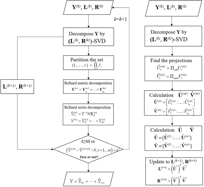
FIGURE 1. Flowchart for IOSSA. The trajectory matrix Y and the left- and right- orthogonal matrix (L, R) of the triple (Y, L, R) is updated by RSVD in left and right panel, respectively.

In the chart, ${\mathcal{T}}^{-1}\mathcal{H}$ denotes the diagonal averaging for the submatrix ${\mathbf{Y}}_{Ji}$ and ${\mathbb{Y}}_{\left(i\right)}^k$ expresses the reconstruction component (RC_Ji) for the k_th iteration. It should be noted that we set L⁰ and R⁰ as identity matrices, meaning that oblique SSA coincides with classical SSA in its first iteration calculation. In this article, three sets of eigentriple numbers in accordance with SSA (see Shen et al., 2017; 2018) are selected, and I = {1, 2, 3, 4, 5, 6, 7} for r = 7 is defined. The chosen set of numbers automatically generates the partition $J_1\bigsqcup J_2\bigsqcup J_3$, representing the trend, Chandler, and Annual periodic components. After a matrix decomposition X = X_J1 + … +X_Jm obtained in the SSA grouping step, we denote Y_Ji = X_Ji (the sub-blocks for Y). By convergence results of (L, R) SVD, the refined RC_Ji will be appointed as

$\left\{\begin{array}{c}R{C}_{\text{trend}}=R{C}_{J1}\\ R{C}_{\text{Chandler}}=R{C}_{J2.}\\ R{C}_{\text{Annual}}=R{C}_{J3}\end{array}\right.(11)$

As another SVD approach, the function of IOSSA to extract the leading components like classical SVD is more appropriate for decomposing the trend and periodic subspaces. In the case of noise pollution, however, the slight edge effects (phase shift) still need to be noteworthy. Furthermore, the IOSSApd with pseudo data is used to address the phase shift issue. First, the original time series PM_ti (1 ≤ i ≤ N) is expanded into PM_tj (1 ≤ j ≤ N + l) by adding pseudo data with a length of l = 365 (day) to the end of the original time series. Expanded by applying the LS + AR model, the pseudo data are assumed to contain a trend, the CW and AW components, and residuals. Thus, the phase shift phenomenon is absorbed in the pseudo data when the expanded time series PM_tj is analyzed using IOSSA. The final deterministic and stochastic components with weak edge effects are obtained by intercepting the first N data (equal length to the original PM_ti sequence).

2.3 Experimental verification

2.3.1 Separability property (case 1)

Here, an example of a short-time series (case 1) is simulated to compare the separability of iterative orthogonal SSA and the common SSA (data length of 10 years; window length: L = 6 years) as

$x_n=A_1\sin \left(2\mathrm{\pi }{f}_1\times t\right)+A_2\sin \left(2\mathrm{\pi }{f}_2\times t\right),(12)$

where t∈[0: 10 years] with the sampling interval of 0.05-year. This synthetic series consisted of two sinusoids. With the same eigenfrequency and average amplitudes of Chandler and Annual wobbles, the f₁ = 1 cpy and f₂ = 0.845 cpy, and A₁ = 1 and A₂ = 1.2 are defined. Figure 2 depicts the result of the SSA decomposition (marked in blue curves). With such close frequencies far from being orthogonal, the SSA cannot separate them for the considered window and series lengths. This completely destroys the structures of periodic signals (e.g., frequency, amplitude, and phase variations) which are clearly visible. The IOSSA algorithm is further applied using two groups, RC_J1 and RC_J2. The iterative operation will be undergone until the convergence result is reached (iterations M = 55). The decomposed results (marked in red curves) confirmed that the proposed method separates harmonics exactly. Therefore, compared with the SSA which is always limited to the components disorder, the application of IOSSA means a higher possibility of such decomposition.

FIGURE 2

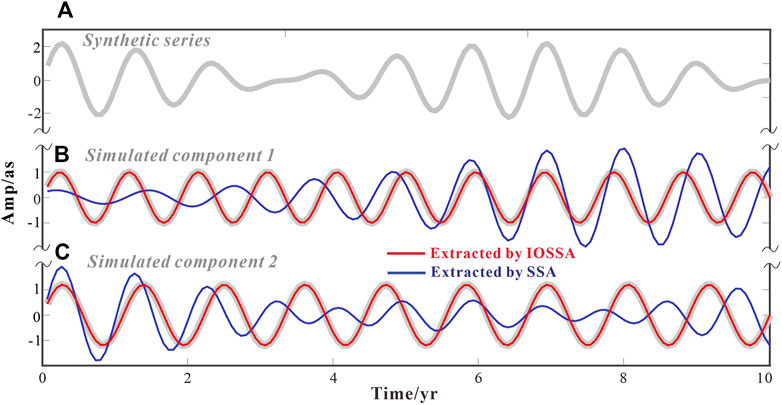
FIGURE 2. Comparison of separation performance between SSA and IOSSA when in the decomposition of sum of sinusoids. (A) Synthetic short-time series (of length 10 years); the extracted component 1 and 2 is shown in (B) and (C).

In reality, when the data-length and sample interval are enough, the SSA can also complete the approximate separation of trend and seasonal terms (Jin et al., 2021). The IOSSA approach, in contrast, has better separation performance even for short-length data. Under heavy noise pollution, the edge effect may become another puzzle, and thus, we designed case 2 to further verify the enhanced IOSSA decomposition with pseudo data.

2.3.2 Edge effect (case 2)

Due to the RCs aliasing, the phase shift at the front/rear ends of the reconstructed trend component will adversely affect the periodic reconstructed component. In this case, the white noise and linear term are added to the simulated case 1. Let us take the data-length as 10 years and L = 6 years again and then

$x_n=A_1\sin \left(2\mathrm{\pi }{f}_{1}n\right)+A_2\sin \left(2\mathrm{\pi }{f}_{2}n\right)+a+bn+{\epsilon }_n.(13)$

By treating sinusoidal amplitudes as A₁ = 1 and A₂ = 1.2, frequencies f₁ = 1 cpy and f₂ = 0.845 cpy, and linear terms for a = 0.8 and b = 0.004, the series is synthesized contained by noise (ε_n variance = 0.35). To show the inhibition effect of the tail effect, the ternary components in case 2 will be restored by IOSSA and IOSSApd, respectively (see Figure 3).

FIGURE 3

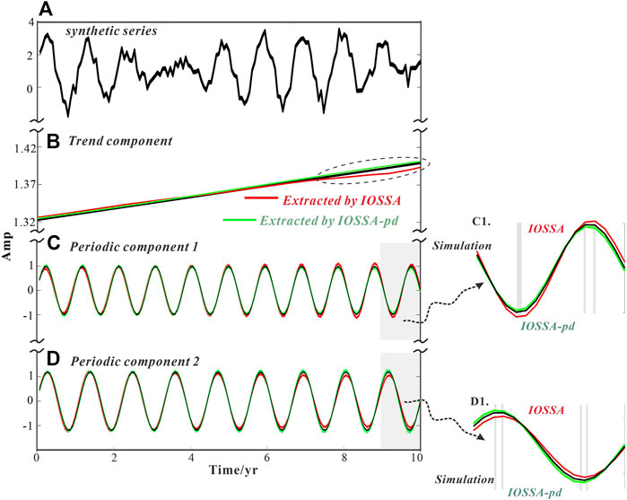
FIGURE 3. Comparison of separation performance between IOSSA and IOSSApd. (A) Synthetic series (of length 150) contained by Gaussian noise; the extracted trend component, periodic component 1 and 2 is shown in (B–D), respectively. C1–D1 indicates the amplification to the rear end of periodic reconstruction, where the light gray domains represent the moment corresponding to the peak or trough.

Figure 3B shows the performance in separating linear components. The unqualified approximation of IOSSA decomposition to the linear term implies the tail effect heavily existing in the trend components (Wang X. et al., 2016). In contrast, we suppressed the phase shift well using the IOSSApd method with extended data at the rear.

In Figure 3C, D, the influence of phase shift in the periodic components is assessed. Under the noise pollution, the offset after IOSSA decomposition and real fluctuation is recorded. At the rear part, the prominent deviation of amplitude (>0.2) or even phase delay (denoted by the gray domain) will contribute an undesirable factor for restoring time series. By contrast, the separated components by IOSSApd can accurately represent periodic reconstructions. Considering their amplitude difference (around 0.06) and full phase-matching does not matter as the fitting degree has increased to a large extent. The previous results show that a more reliable principal component can be produced by solving the phase shift problem with the IOSSApd method.

3 PM analysis

3.1 Data source

Covering 1 January 1962–31 December 2021, the EOP 14 C04 PM time series are provided by IERS. The IERS supported the 1-day solution files by radio-positioning integrated by DORIS, GNSS, VLBI, and SLR with a precision of 0.02 mas (Liu et al., 2009; Bizouard et al., 2019). Consistent with the conventional reference frame ITRF 2014, the PM dataset can be accessed at https://www.iers.org/IERS/EN/DataProducts/EarthOrientationData/eop.html.

3.2 Non-stationary trend

In the traditional LS-based forecast, the linear fitting for a non-stationary trend was reconsidered as unscientific and will introduce a predicted error of more than 10 mas. The visible secular variations appear in the polar motion measured with multi-geodetic techniques (e.g., SLR, VLBI, GNSS, and DORIS). The IOSSA analysis gives the x and y components for PM from 1962 to 2021, which departs away from zero (see Figure 4). In Figure 4A, the polar motion refers to the CIO frame (x for PM: south direction; y for PM: west direction). The trend drift (PM secular rate (per year) in polar-coordinate) rates in the decadal and centurial scales are presented in the first and second quadrants, respectively. In the decades scale, the trend rate of the PM varies from 2.56 ± 0.0714 mas to 7.73 ± 0.0286 mas per year. The linear velocity of trend drift narrates that the Earth’s polar motion speeds up in the latest decade (2010–2019) (see Figure 4B), which is different from the slowing in the geologic age. It reveals the long-term fluctuation in the Earth’s polar motion (Guo and Han 2009). In the century-scale, the rate and direction of PM from different authors were given (Markowitz 1968; Wilson and Vicente, 1980; McCarthy and Luzum 1996). The trend rate of pole motion is from 3.2 to 3.4 mas per year with the well-known direction of Greenland. However, the trend rates of PM in the X and Y directions in Figure 4B, covering over half of the century, are 2.01 ± 0.1819 and 3.11 ± 0.2021 mas per year. The North Pole moves to 57.1 °E in the longitude direction concerning the crust. The Barents Sea is fit in this direction. These different results also implied that the non-linear drift contains some unmistakable low-frequency signals, and the accurate separation of trend components for fitting and extrapolating is necessary.

FIGURE 4

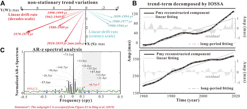
FIGURE 4. Drift trend of polar motion. (A) Variations of polar motion in the decade (red arrows) and century (blue arrows) scales in previous studies, (B) non-stationary trend component decomposed by IOSSA, and (C) AR-z spectral analysis for interdecadal signals by Ding et al. (2019).

The complex composition of PM oscillation from interdecadal to even century-scale has been researched by Ding et al. (2019). In Figure 4C, according to the AR-z spectrum, a robust weak signal recognizer with high spectral resolution than the conventional Fourier-based spectrum, the complex time series (x + iy) in a low-frequency band is explored. The nine spectral peaks in the –0.1∼+0.1 cpy band, and the corresponding periods are approximately –17.1 years, –26.5 years, –50.8 years, –166.7 years, +73.5 years, +33.8 years, +17.1 years, +13.8 years, and +11.4 years, meaning the trend drifts with intense time-varying characteristics. Some of these multi-spectral peaks in the frequency domain have been identified as the consistent geophysical periodicities from, e.g., the solar cycle (∼11 years) (Currie, 1981), the Earth’s nutation (∼33 years and ∼14 years) (Ding and Chao, 2018), geomagnetic variations (∼28 years, ∼50 years, and ∼70 years) (Dickey and Viron, 2009; Dobrica et al., 2018), and others perhaps induced from atmospheric or oceanic effects (Ding et al., 2019). Integrating with the upgraded SSA separator (iterative oblique SSA) and multiple-harmonic models, the non-stationary trend-terms are first reconstructed and then fit completely with these low-frequency signals (see Figure 4B, fitting residual <1 mas). In the following context, such long-period oscillation extrapolation is considered as the initial trial.

4 Prediction procedure

One limitation of SSA is the significant biases in the beginning and end of its model fitting to a time series called phase phenomenon (Wang X. et al., 2016). To address the phase shift phenomenon and improve the PM forecast, we proposed the IOSSApd method in the frame of a two-step strategy. By adhering to the predictions of the LS + AR (initial) model to the end of the PM series, the IOSSA (enhanced version of SSA) will give a formidable oscillation separation. After the MH + ARIMA model (terminal) triggered the second cycle forecast, the final RC predictions (RCPs) will be produced. By this proposed hybrid method, 11 years of PM predictions were made at 12-month intervals from 1 January 2010, and the main steps (see Figure 5) are as follows:

i. Pseudo data (-pd). In pseudo prediction, the LS + AR model is commonly used to predict the Earth’s orientation parameters with simple construction and lower accuracy (Kalarus et al., 2010). Here, we fit and forecast the linear and periodic terms (L = 365 days), including Chandler wobble and annual wobble, and the AR model matches semi-annual periodic terms in PM and their remnants. The predicted series by LS + AR is attached to the end of PM observations as pseudo data with a total length of N + L.

ii. IOSSA decomposition. By high-precision observation (1962), the long-term PM series (of length N + L) with LS + AR predictions at the end is separated by IOSSA. According to the partition of $J_1\bigsqcup J_2\bigsqcup J_3$ and chosen window of 2190 points, the deterministic components of trend (RC_J1), the Chandler wobble (RC_J2), and the annual wobble (RC_J3) are obtained with the stochastic component remaining. For each component, a hybrid model of MH or ARIMA is adopted under different coverage to make a precise extrapolation.

iii. Final prediction. The PM series has been recognized as multifrequency modes from the interannual, short-term (e.g., seasonal) oscillations to the long-term trend. The time-varying oscillation can be precisely approximated and extrapolated by the sinusoids in frequency-amplitude modulation. A modified LS model, a multiple-harmonic (MH) model, is creatively proposed in the system of equations as

$\left\{\begin{array}{l}P{M}_{\text{Annual}}\left(t\right)=\left(a_A+m_{A}t\right)\sin \left(2\mathrm{\pi }{f}_{A}t+w_A\right),\\ P{M}_{\text{Chandler}}\left(t\right)={\displaystyle \sum _{i=1}^M}{b}_{Ci}\sin \left(2\mathrm{\pi }{f}_{Ci}t+w_{Ci}\right),\\ P{M}_{\text{Trend}}\left(t\right)={\displaystyle \sum _{i=1}^N}{b}_{Ti}\sin \left(2\mathrm{\pi }{f}_{Ti}t+w_{Ti}\right),\\ P{M}_{\text{Tide}}\left(t\right)={\displaystyle \sum _{i=1}^P}{b}_{TDi}\sin \left(2\mathrm{\pi }{f}_{TDi}t+w_{TDi}\right).\end{array}\right.(14)$

FIGURE 5

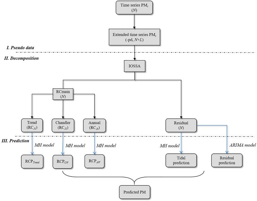
FIGURE 5. Flowchart of the IOSSApd + MH + ARIMA method for PM prediction.

In Eq. (14), the $a_A$ and $m_A$ are the constants of the annual linear amplitude (Shen et al., 2018), f_A = 1/365.25 is the annual frequency, and $w_A$ is the un-estimated phase. Instead of the assumption of an initial constant period (e. g., 428 days) in the biaxial rigid Earth (Becker, 1954), the later double-periods motion (e.g., 428 and 438 days) with the beat model (Colombo and Shapiro, 1968) or the recent variable period (e.g., from 392 to 441 days) under the sustained excitation (Wang G. et al., 2016), the MH fitting for CW was postulated as 5-period channels (namely, M = 5, Pan. 2007; Zhang et al., 1986) of T_main {432 days}, T_1,0 and T_1,1 {symmetrical peaks: 429 and 435 days}, and T_2,0 and T_2,1{symmetrical peaks: 406 and 447 days}. These multiple Chandler frequencies correspond to the parameter f_C1–f_C5, respectively, and consist of a fundamental frequency attributable to the Earth’s triaxiality, a series of small feedback frequencies arising from the Earth’s instantaneous inertia, relative angular momentum, and inertia variation. In the triaxial Earth model, the Chandler wobble may behave like a multiple-coupling differential oscillation with the mantle as the major and permanent coupler. Such a multiple-frequency model can explain the Chandler amplitude and frequency variations with time (for more details about the observed CW frequency-splitting and validation, please see Pan (2007; 2012)). According to Xu (2013), the sampling for both components covers 9 years (7.6 Chandler periods or 9 annual terms). In addition, the MH model was applied for the first time in forecasting non-stationary trends as long-period oscillations (N = 9) and tidal harmonics as seasonal oscillations (p = 7). The dominant frequency (f_T1–f_T9, please refer to Figure 4) and (f_TDi) parameter (f_TD1–f_TD7, please refer to Chin et al. (2004)). In addition to these multiple deterministic components, the stochastic components (containing quasi-periodic signals) are also considered. In this article, for the stochastic sequence, a more stable and robust sequence is obtained by ARIMA than an AR or ARMA model in the case of the modeling of a seasonal differential operator as

$y_t={\theta }_0+{\varphi }_1{y}_{t-1}+{\varphi }_2{y}_{t-2}+\cdots +{\varphi }_p{y}_{t-p}+{\epsilon }_t-{\theta }_1{\epsilon }_{t-1}-{\theta }_2{\epsilon }_{t-2}-\cdots -{\theta }_q{\epsilon }_{t-q}.(15)$

The model is usually described as ARIMA (p, k, q). The ternary orders of p, k, and q offsetting the tide effect (Chin et al., 2004) are estimated using the least squares method. Combining the predictions from the multi-harmonic and ARIMA (p, q, k) model will yield the final results. When the adjacent period changes, their time-varying characteristics can be fully reflected in 1-year PM predictions.

5 Predictions of the polar motion

5.1 The predicted results and precision comparison

In this study, EOP 08 C04 PM data from 1962 to 2021 were selected for the validation of SSApd + MH + ARIMA predictions. The PM from 1 January 1964 to the predicted start time was used as the original PM series. After IOSSApd decomposition, the principal components of 1-year lead time PMs (denoted as PCP) were predicted using the MH (5-period channels CW + linear AW + non-stationary trend, see Eq. 14) and the LS model (sinusoid CW/AW + linear trend, refer to Shen et al., 2017), respectively. We produced multiple sets of predicted PMs in 1-year-leading (of 2010–2021 years). Decomposition of the original PM series concerning the prediction period was also performed by IOSSApd to obtain the real principle components (denoted by PC). The predictive errors (PC-PCP) for all prediction periods are shown in Figure 6.

FIGURE 6

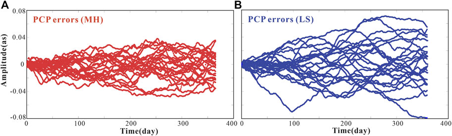
FIGURE 6. Predictive errors of PM principle components (Chandler + annual + trend) using (A) MH model and (B) LS model in both the x/y poles.

Figure 6 shows that the PCP series obtained by the MH model are more consistent with the original PCs over multiple prediction periods than the conventional LS model (errors: ±40 mas in random variations. vs. ±70 mas in periodic fluctuation). The trend, annual, and Chandler terms contribute most of the energy of polar motion; therefore, the MH predictor will produce the satisfied principle components that accurately represent the original series, ARIMA. Concerning the residual IOSSApd series, we mainly used the ARIMA to extrapolate them (see Figure 5). The extrapolation results of the ARIMA model were combined with the principle component predictions of the MH (ARIMA + MH) to yield the whole 1-year PM predictions.

The predictions of Bulletin A including PM parameters for 1 year into the future were provided by IERS and are currently recognized as the official forecasts, which relied on the history observations (Stamatakos et al., 2011). To verify the reliability of the IOSSApd + MH + ARIMA method, the accuracy of the predicted series was compared with the accuracy of the IERS Bulletin A predictions (http://datacenter.iers.org/eop/-/somos/5Rgv/getTX/6). As shown in Figure 7, the systematic prediction of both methods can be seen. With a relatively high precision in the 180-day forecast, the IOSSApd + MH + ARIMA’s prediction is even more accurate in the 365-day forecast than the Bulletin A. It indicated the proposed solution predicting the PM parameters precisely and effectively. As the comparable results from the IERS Bulletin A, the combination of the IOSSApd and ARIMA produced PM series with a higher consistency of observations in most cases. The better performance of the IOSSApd + MH + ARIMA prediction was attributed to the modeling of frequency- and amplitude-modulation for the Chandler, the annual oscillation, and the superposition of non-stationary trend.

FIGURE 7

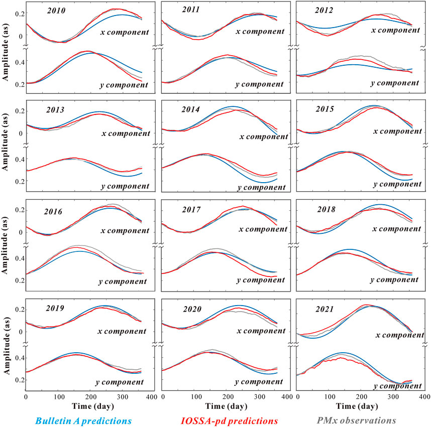
FIGURE 7. From the epoch of 2010 to 2021 years, the polar motion series (gray line), the IERS “Bulletin A” predictions (blue line), and the IOSSA + MH + ARIMA predictions (the red line) in 1-year leading.

Figures 8A,C indicate that in the leading 1-year predictions, the mean absolute errors (MAEs) of our proposed two-step forecast were lower since the 50th day than the predictions reported routinely in Bulletin A. In particular, the IOSSApd + MH + ARIMA’s predictive accuracy at forecast horizons of 180-day to 360-day was significantly higher over the Bulletin A. Corresponding to improvements of 28.89% for y-pole, the remaining prediction errors for x-pole are even more minor with the advancements of 35.60%. The MAEs are shown in Table 1. In the 180-day predictions, the MAEs of IOSSApd + ARIMA for the x and y components are 10.85 and 8.78 mas, respectively, smaller than those of 14.83 and 11.31 mas for the Bulletin A predictions. In the 360-day predictions, the MAEs for x and y components from IOSSApd + MH + ARIMA were 12.03 and 13.93 mas, respectively, much smaller than those of 18.68 and 19.59 mas for Bulletin A. The MAE of IOSSApd + MH + ARIMA increased slowly with the increase in the forecasting time, and the prediction accuracy of 360 was several mas more than that of 180 days. This implied that the forecasting errors in the 180–360 days are limited to a small range. The IOSSA can reliably reconstruct the stable principal components fitting by multispectral peak or time-varying amplitude harmonics. It enables the IOSSApd + MH + ARIMA to be particularly suitable for long-term prediction. Moreover, at the entire forecast horizons, the mean absolute error of IOSSApd + MH + ARIMA prediction was generally less than 12 mas and 15 mas for x and y components, respectively; while in the Bulletin A predictions, the time interval at equal accuracy only covers 1–130 days and 1–260 days, respectively. As for the short-term prediction within 50 days, high-frequency oscillation (or quasi-periodic oscillations) and random residual are still tricky because this article mainly refined the mid-term and long-term prediction of x/y-pole and the ultra-to fast-forecast is not discussed.

FIGURE 8

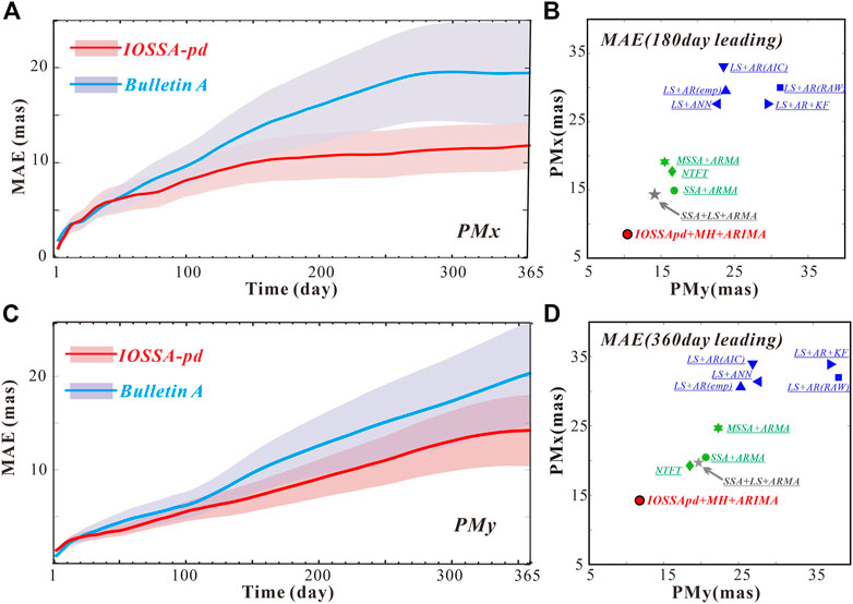
FIGURE 8. MAE of the IERS Bulletin A (red) and IOSSA + ARIMA predictions (blue) in x-component (A) and y-component (C). MAE of the predictions by other methods in 180-day (B) and 360-day (D) leading. The shadows represent the error domain.

TABLE 1

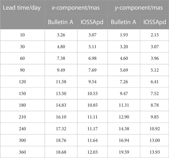
TABLE 1. Comparison of the MAE of IERS Bulletin A and IOSSApd + MH + ARIMA predictions.

The MAE of the 180-day and the 360-day leads were also compared with the results of other methods (see Figures 8B,D). We classified these methods into two categories: the LS-based methods (marked in purple) and time-variant methods (marked in green). The former include the LS + AR, LS + AR + AF, and LS + ANN methods (Kosek et al., 2007; Liao et al., 2012; Jia et al., 2018; Sun et al., 2019), which relied upon the fixed-frequency and linear trend, and another group consisted of NTFT, MSSA + ARMA, and SSA + ARMA methods (Su et al., 2014; Shen et al., 2018; Jin et al., 2021), the algorithm dominated by decomposed non-stationary components. Evidently, the MAEs of PM with the time-variants method were significantly less than those of LS-based methods, either in the middle- or long-prediction. Notably, the SSA + LS + ARMA predictive model [marked in gray, Shen et al. (2017)] adopts a similar strategy to the IOSSApd + MH + ARIMA method, i.e., the decomposition from polar motion observations first and fitting-extrapolation (but in single Chandler harmonic at Tcw = 432 days) second to achieve a high-precise prediction (MAE<15 mas in middle-term, and <20 mas in long-term for x/y-poles). Compared with these methods, we examined the multi-frequency points/band in IOSSApd’s reconstructed components and, hence, improved the predictive performance to a large extent.

5.2 The periodic errors analysis

When the PM predicted errors are accumulated with leading time, they are always clustered and manifested in the pattern of periodic errors. These periodic errors can be used as indicators for analyzing the forecast accuracy of periodic/quasi-periodic components. In this section, the absolute error (AE) comparisons against the general SSA-based method (SSA + MH + ARIMA, the same window of 6 years, and the predictive component of the first 7th RC as IOSSA) for the 1-year-leading PM prediction are further conducted in the same span of 2010–2021. In Figure 9, a typical high-error presentation with different patterns, e.g., from 2014 to 2016, which was heavily affected by the super El Niño action, is analyzed. As the NOAA National Centers for Environmental Information’s State of the Climate report states, the El Niño recorded was the most prolonged in duration and the most vigorous in intensity since the comprehensive observations emerged in September 2014 and dissipated in May 2016. The circulation pattern and temperature anomaly promote the amplitude variations of the annual wobble (Coulot and Pollet, 2010). Correspondingly for SSA + MH + ARIMA, the predicted error increased with –6–65 mas (July–December 2014), –23–50 mas (September–December 2015), and −10–41 mas (February–June 2016) for the y-pole prediction. Advanced by ∼120 days phase lead-lag, the predicted error in the x-pole also spread within ±50 mas, implying the prominent periodic residuals. Such error clusters covering even over half a year are a widespread occurrence in the 12-year PM predictions. Failure to trace the time-variant periodic term (annual and Chandler wobbles), here for SSA, is evidenced adequately. In contrast, the IOSSApd + MH + ARIMA’s reduction ability is excellent, either in error clusters timespan or its intensity. Based on the amplitude–frequency modulation, the extended conditions of the x/y-pole multi-components in high separation play a crucial role in the successful forecast.

FIGURE 9

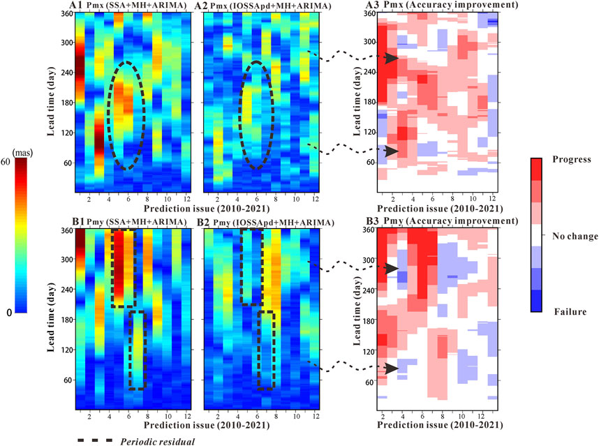
FIGURE 9. Absolute errors of the predicted x-component (A2) and y-component (B2) for the 2010–2021 years, compared with those of the SSA + MH + ARIMA model [(A1) and (B1)]. The black box represents the El Niño event as an epoch example when the error cluster is piled up with periodic residuals. The right panels show the improvement of x/y-pole prediction using the IOSSApd + MH + ARIMA model compared with the SSA + MH + ARIMA in x-component (A3) and y-component (B3), where the progress (red), no change (white) and failure (blue) reflects the difference of both predicted error >5 mas, within ±5, and <5 mas, respectively. The darker the color, the greater their difference is.

The heat maps are drawn (Figure 9A3 and B3) to better understand such a periodic error in the mid- and long-term forecast to demonstrate the predicted improvement in the IOSSApd + MH + ARIMA solution compared to SSA + MH + ARIMA. For each prediction epoch, if the difference between predicted errors of IOSSApd + MH + ARIMA and SSA + ARMA is within ±5 mas, it cannot be regarded as an improvement in prediction. As illustrated in the white blocks in Figures 9B and D, the error amounted to the same level for both PM prediction techniques. If the difference >5 mas, the IOSSA-pd + MH + ARIMA prediction was considered to have a smaller error than SSA + ARMA and marked by red blocks. In other cases, the failure in the prediction process was denoted by blue blocks. The large improved areas (red) demonstrated that the behavior of PM prediction is progressed by IOSSA-pd + MH + ARIMA, especially in long time intervals.

By the ratio of the colored area (white + red) to the total area (white + red + blue) in each epoch, we introduced the success rate of PM prediction. Table 2 shows the success rate of 2010–2021 using the IOSSApd + MH + ARIMA algorithm. On average, the success rate of the x and y components surged to 70.82% and 74.02%, respectively, and the improvement in the PM prediction reached approximately 73%. Therefore, our predicted PM results reflect weaker and smoother periodic errors in mid- and long-term predictions, and this is largely because the IOSSApd separator performs better in reconstructing the PC series than the general SSA.

TABLE 2

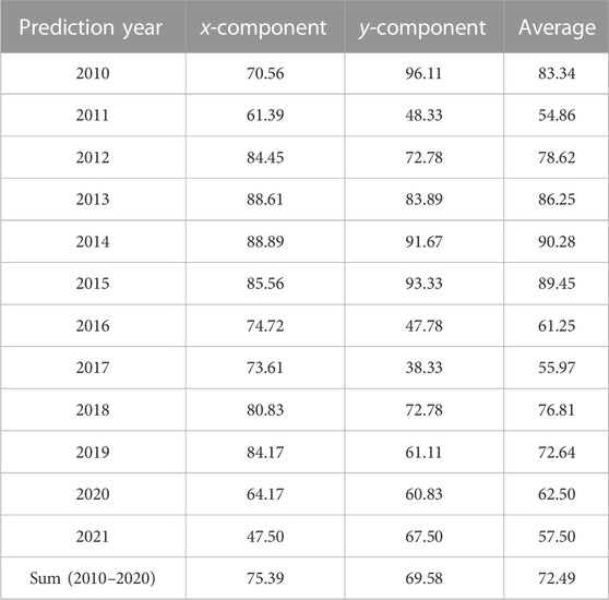
TABLE 2. Success rate for PM (no change + progress).

Based on the experiments covering the years 2010–2021, comprehensive prediction errors were collected by additional statistics to verify the compliance of the normal distribution. In Figure 10, the error distribution features by IOSSApd + MH + ARIMA and SSA + MH + ARMA are shown, and their error curves are also drawn.

FIGURE 10

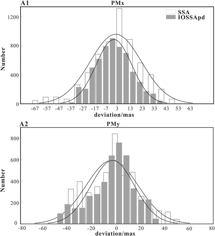
FIGURE 10. Distributions of the IOSSA + MH + ARIMA (gray) and SSA + MH + ARIMA (white) prediction residuals with the best-fitted normal distributions in x-pole (A1) and y-pole (A2).

By reducing the effect of the phase shift in each prediction epoch, the two-step solutions might be superior and then in the presentation of a Gaussian-like rule. To exactly describe the time series as reasonably Gaussian, four statistical parameters were introduced, including mean value (μ), standard deviation (σ), skewness (s), and excess kurtosis (k). As for the μ and σ parameters, they provided the quantitative reference defining the location and aggregation of the error distribution. Else, for the s and k estimators, they indicate the state or quality of asymmetry and peakedness (or flatness), describing the normal distribution error in the region about its mode. According to Tabachnick et al. (2007), these parameters are formulated as follows:

${\widehat{\mu }}_i=\frac{1}{n_p}{\displaystyle \sum _{j=1}^{n_p}}{\epsilon }_{i,j},\hspace{1em}{\widehat{\sigma }}_{{\widehat{\mu }}_i}=\frac{{\widehat{\sigma }}_i}{\sqrt{n_p}},(17)$

${\widehat{\sigma }}_i=\sqrt{{\displaystyle \sum _{j=1}^{n_p}}\frac{{\left({\epsilon }_{i,j}-{\widehat{\mu }}_i\right)}^2}{n_p-1}},\hspace{1em}{\widehat{\sigma }}_{{\widehat{\sigma }}_i}=\frac{{\widehat{\sigma }}_i}{\sqrt{2n_p}},(18)$

${\widehat{s}}_i={\displaystyle \sum _{j=1}^{n_p}}\frac{{\left({\epsilon }_{i,j}-{\widehat{\mu }}_i\right)}^2}{\left(n_p-1\right){\widehat{\sigma }}_i^2},\hspace{1em}{\widehat{\sigma }}_{{\widehat{s}}_i}=\sqrt{\frac{6}{n_p}},(19)$

${\widehat{k}}_i={\displaystyle \sum _{j=1}^{n_p}}\frac{{\left({\epsilon }_{i,j}-{\widehat{\mu }}_i\right)}^4}{\left(n_p-1\right){\widehat{\sigma }}_i^4}-3,\hspace{1em}{\widehat{\sigma }}_{{\widehat{k}}_i}=\sqrt{\frac{24}{n_p}}.(20)$

Next, the prediction error distribution of the PM time series is characterized in detail. As listed in Table 3, the μ value (−1.5 mas and −2.0 mas for the x/y pole) of IOSSApd + MH + ARIMA evidenced that this algorithm offers a solution approximating the unbiased estimation, meaning the prediction errors are close to zero. The second parameter σ plays another vital role in the quality of the prediction and is related to the error range and limits. Regarding the estimator, the IOSSApd (σ = 14.1 mas on average) is still more competitive than SSA (σ = 21.3 mas on average).

TABLE 3

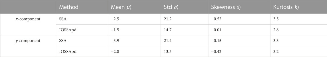
TABLE 3. Statistical index of Gaussian distribution in Figure 10.

Using the skewness and the kurtosis parameters, other interesting explorations can be performed. On one hand, the s parameter in both methods all have a positive value (the right tail is stronger than the left one) for the x-pole and a negative value for the y-pole (the right tail is weaker than the left one). On the other hand, the positive value of the k parameter for each pole implies that the distribution is peaked relative to a normal one. Specific to each method, the periodic signals of predicted error by IOSSApd + MH + ARIMA decreased rapidly. When compared with SSA + MH + ARIMA (|s| = 0.34, k = 3.4 on average), these errors (|s| = 0.21, k = 3.0 on average) are more statistically normal significant because of their smaller parameter values (except for the skewness in y-pole).

6 Conclusion

In this article, we introduce a newly improved separator (iterative oblique SSA) used in the decomposition of deterministic components. The Chandler wobble, annual wobbles, or even the non-stationary trend of the Earth’s polar motion can be considered as quasi-harmonic processes, as indicated by the IOSSA. To reduce the phase shift, a two-step strategy (pseudo date in initial prediction by LS + AR) is preliminarily established, called IOSSApd. Based on the IOSSApd decomposition, many periodic/quasi oscillations in interdecadal and decadal (trend term), as well as inter-to sub-annual (CW, AW, tidal, and seasonal) scales, were involved in obtaining a routinely high-accuracy PM prediction for up to 1-year into the future. When compared to other forecast products, the main advantages of IOSSApd + MH + ARIMA predictions are listed as follows:

• The extended separation conditions than classical SVD decomposition.

• The generation of pseudo data (PD) to address the tail effect.

• Long-period superposition of interdecadal oscillations instead of conventional (non) linear trend.

• Amplitude and frequency modulation by multispectral peaks for Chandler and annual wobbles.

• Robust process for high-frequency residuals by seasonal difference operator.

Using the Bulletin A published in IERS as a reference (predictions set to 1 year into the future, 2010–2021 on experiments), multiple sets of the predicted performance were elaborated. The forecasts of IOSSApd + MH + ARIMA were almost equal to the IERS Bulletin A within the 50th-day projections, while after that, notable promotions were recorded. As forecast time increased, the prediction error accumulated slowly until the 1-year lead time. At the entire forecast horizon, the remaining prediction errors were approximately 12 mas and 14 mas for PM, respectively, corresponding to significant improvements of 35.60% and 28.89% for x and y poles over Bulletin A. Some common patterns, e.g., the El Niño effect or geomagnetic jerk events, might excite the time-variant Chandler and annual wobbles and cause high cluster errors. Interestingly, whether it is the time span or the intensity of the periodic remaining, the inhibition capability of IOSSApd + MH + ARIMA is pretty impressive. In terms of the daily improvement for the x and y poles, our multivariate algorithm was found to reach up to 75.39% and 69.58% in the 1-year leading predictions, respectively. These results exhibit the excellent consistency of the predicted and original PM periods’ periodic and trend terms. Based on the collected prediction error, the PM predictions were finally evaluated by normal distribution statistics. The Gaussian-like distribution further implies by the IOSSApd + MH + ARIMA method; the PM principal components can be sufficiently extracted and extrapolated with tiny oscillatory residuals (interannual or interdecadal). Therefore, our proposed method has good reliability and high precision for this PM prediction. Finally, although the IOSSApd + MH + ARIMA method developed in the study is most suitable for middle- and long-term PM forecasts, one can also extend our multivariate algorithm to forecast other EOP parameters by considering the different multiple periods in it.

Data availability statement

The original contributions presented in the study are included in the article/Supplementary Material; further inquiries can be directed to the corresponding author.

Author contributions

KS was involved in the advanced multivariate algorithm, drawing images, and conducting the manuscript writing. HD contributed to the PM predictions design and manuscript proof reading. CZ and TC helped in collecting PM and Bulletin A datasets. All authors read and approved the final manuscript.

Funding

This study is supported by the National Natural Science Foundation of China (Grants: 41974022, 41721003, and 42192531), Educational Commission of Hubei Province of China (Grant: 2020CFA109), and the Project Supported by the Special Fund of Hubei Luojia Laboratory (Grant: 220100002).

Acknowledgments

The authors thank IERS for providing IERS 14 C04 polar motion series and Bulletin A, which can be obtained for free by downloading from https://www.iers.org/IERS/EN/DataProducts/EarthOrientationData/eop.html. The IOSSA method was performed using the R Language, available at https://rdrr.io/cran/Rssa/man/iossa.html.

Conflict of interest

The authors declare that the research was conducted in the absence of any commercial or financial relationships that could be construed as a potential conflict of interest.

Publisher’s note

All claims expressed in this article are solely those of the authors and do not necessarily represent those of their affiliated organizations, or those of the publisher, the editors, and the reviewers. Any product that may be evaluated in this article, or claim that may be made by its manufacturer, is not guaranteed or endorsed by the publisher.

References

Akyilmaz, O., and Kutterer, H. (2004). Prediction of Earth rotation parameters by fuzzy inference systems. J. Geod. 78, 82–93. doi:10.1007/s00190-004-0374-5

CrossRef Full Text | Google Scholar

Akyilmaz, O., Kutterer, H., Shum, C. K., and Ayan, T. (2011). Fuzzy-wavelet based prediction of Earth rotation parameters. Appl. Soft Comput. 11, 837–841. doi:10.1016/j.asoc.2010.01.003

CrossRef Full Text | Google Scholar

Barnes, R., Hide, R., and Wilson, A. (1983). Atmospheric angular momentum fluctuations, length-of-day changes and polar motion. Proc. R. Soc. Lond. B. Biol. Sci. 387, 31–73. doi:10.1098/rspa.1983.0050

CrossRef Full Text | Google Scholar

Becker, R. A. (1954). Introduction to theoretical mechanics. McGraw-Hill, New York.

Google Scholar

Bizouard, C., Lambert, S., Gattano, C., Becker, O., and Richard, J. Y. (2019). The IERS EOP 14C04 solution for Earth orientation parameters consistent with ITRF 2014. J. Geod. 93, 621–633. doi:10.1007/s00190-018-1186-3

CrossRef Full Text | Google Scholar

Buffett, B., Mathews, P. M., Herring, T. A., and Shapiro, I. I. (1991). Forced nutations of the Earth: Influence of inner core dynamics, 4, Elastic deformation. J. Geophys. Res. Atmos. 96, 8258–8274.

CrossRef Full Text | Google Scholar

Chandler, S. C. (1891). On the variation of latitude, I. Astron. J. 11, 59–61. doi:10.1086/101603

CrossRef Full Text | Google Scholar

Chao, B. F., and Chung, W. Y. (2012). Amplitude and phase variations of Earth's Chandler wobble under continual excitation. J. Geodyn. 62, 35–39. doi:10.1016/j.jog.2011.11.009

CrossRef Full Text | Google Scholar

Chen, J. L., and Wilson, C. R. (2005). Hydrological excitations of polar motion, 1993–2002. Geophys. J. Int. 160, 833–839. doi:10.1111/j.1365-246X.2005.02522.x

CrossRef Full Text | Google Scholar

Chin, T. M., Gross, R. S., and Dickey, J. O. (2004). Modeling and forecast of the polar motion excitation functions for short-term polar motion prediction. J. Geod. 78, 343–353. doi:10.1007/s00190-004-0411-4

CrossRef Full Text | Google Scholar

Colombo, G., and Shapiro, I. I. (1968). Theoretical model for the Chandler wobble. Nature 217, 156–157. doi:10.1038/217156a0

CrossRef Full Text | Google Scholar

Coulot, D., Pollet, A., Collilieux, X., Berio, P., Collilieux, X., and Berio, P. (2010). Global optimization of core station networks for space geodesy: Application to the referencing of the SLR EOP with respect to ITRF. J. Geod. 84, 31–50. doi:10.1007/s00190-009-0342-1

CrossRef Full Text | Google Scholar

Currie, R. G. (1981). Solar cycle signal in Earth rotation: Nonstationary behavior. Science 211, 386–389. doi:10.1126/science.211.4480.386

PubMed Abstract | CrossRef Full Text | Google Scholar

Dicke, J. O., and Viron, O. (2009). Leading modes of torsional oscillations within the Earth's core. Geophys. Res. Lett. 36, L15302. doi:10.1029/2009GL038386

CrossRef Full Text | Google Scholar

Ding, H., and Chao, B. F. (2018). Application of stabilized AR-z spectrum in harmonic analysis for geophysics. J. Geophys. Res. Solid Earth 123, 8249–8259. doi:10.1029/2018JB015890

CrossRef Full Text | Google Scholar

Ding, H., Pan, Y. J., Xu, X. Y., and Li, M. (2019). Application of the AR-z spectrum to polar motion: A possible first detection of the inner core wobble and its implications for the density of Earth's core. Geophys. Res. Lett. 46, 13765–13774. doi:10.1029/2019GL085268

CrossRef Full Text | Google Scholar

Dobrica, V., Demetrescu, C., and Mandea, M. (2018). Geomagnetic field declination: From decadal to centennial scales. J. Geophys. Res. Solid Earth 9, 491–503. doi:10.5194/se-9-491-2018

CrossRef Full Text | Google Scholar

Golyandina, N., and Shlemov, A. (2013). Variations of singular spectrum analysis for separability improvement: Non-orthogonal decompositions of time series. Stat. Interface 8, 277–294. doi:10.4310/SII.2015.v8.n3.a3

CrossRef Full Text | Google Scholar

Gross, R. S. (2007). Earth roation variations-long period, in Physical geodesy, edited by T. A. Herring, Elsevier, Amsterdam, in press.

Google Scholar

Gross, R. S., Fukumori, I., and Menemenlis, D. (2003). Atmospheric and oceanic excitation of the Earth's wobbles during 1980–2000. J. Geophys. Res. Solid Earth 108, 2370–2385. doi:10.1029/2002JB002143

CrossRef Full Text | Google Scholar

Guo, J., and Han, Y. (2009). Seasonal and inter-annual variations of length of day and polar motion observed by SLR in 1993–2006. Chin. Sci. Bull. 54, 46–52. doi:10.1007/s11434-008-0504-1

CrossRef Full Text | Google Scholar

Hinderer, J., Legros, H., Gire, C., and Le Mouël, J. L. (1987). Geomagnetic secular variation, core motions and implications for the Earth's wobbles. Phys. Earth. Planet. 49, 121–132. doi:10.1016/0031-9201(87)90136-1

CrossRef Full Text | Google Scholar

Jia, S., Xu, T., and Yang, H. (2018). Two improved algorithms for LS+AR prediction model of the polar motion. Acta Geod. Cartogr. Sinica 47, 71–77. doi:10.11947/j.AGCS.2018.20180296

CrossRef Full Text | Google Scholar

Jin, X., Liu, X., Guo, J., and Shen, Y. (2021). Analysis and prediction of polar motion using MSSA method. Earth Planets Space 73, 147. doi:10.1186/s40623-021-01477-2

CrossRef Full Text | Google Scholar

Kalarus, M., Schuh, H., Kosek, W., Bizouard, C., and Gambis, D. (2010). Achievements of the Earth orientation parameters prediction comparison campaign. J. Geod. 84, 587–596. doi:10.1007/s00190-010-0387-1

CrossRef Full Text | Google Scholar

Kosek, W. (2012). “Future improvements in EOP prediction,” in Geodesy for planet earth. International association of geodesy symposia vol 136. Editors S. Kenyon, M. Pacino, and U. Marti (Berlin, Heidelberg: Springer). doi:10.1007/978-3-642-20338-1_62

CrossRef Full Text | Google Scholar

Kosek, W., Kalarus, M., and Niedzielski, T. (2007). “Forecasting of the earth orientation parameters: Comparison of different algorithms,” in Proceedings of the Journèes systems de dereference spatio-temporels, Observatoire de Paris, Paris, France, 17–19 Sept 2007. pp155–158.

Google Scholar

Kosek, W., Mccarthy, D. D., and Luzum, B. J. (1998). Possible improvement of Earth orientation forecast using autocovariance prediction procedures. J. Geod. 72, 189–199. doi:10.1007/s001900050160

CrossRef Full Text | Google Scholar

Liao, D. C., Wang, Q. J., Zhou, Y. H., Liao, X. H., and Huang, C. L. (2012). Long-term prediction of the Earth orientation parameters by the artificial neural network technique. J. Geodyn. 62, 87–92. doi:10.1016/j.jog.2011.12.004

CrossRef Full Text | Google Scholar

Liu, L., Hsu, H., Gao, B., and Wu, B. (2000). Wavelet analysis of the variable Chandler wobble. Geophys. Res. Lett. 27, 3001–3004. doi:10.1029/1999GL011094

CrossRef Full Text | Google Scholar

Liu, W., Li, Z., Liu, W., and Wang, F. X. (2009). Influence of EOP prediction errors on orbit prediction of navigation satellites. GNSS World China 34, 17–22. doi:10.13442/j.gnss.2009.06.010

CrossRef Full Text | Google Scholar

Malkin, Z., and Miller, N. (2010). Chandler wobble: Two more large phase jumps revealed. Earth Planets Space 62, 943–947. doi:10.5047/eps.2010.11.002

CrossRef Full Text | Google Scholar

Markowitz, W. (1968). Concurrent astronomical observations for studying continental drift, polar motion, and the rotation of the Earth. Netherlands: Springer.

Google Scholar

McCarthy, D. D., and Luzum, B. J. (1996). Path of the mean rotational pole from 1899 to 1994. Geophys. J. Int. 125, 623–629. doi:10.1111/j.1365-246X.1996.tb00024.x

CrossRef Full Text | Google Scholar

Modiri, S., Belda, S., Heinkelmann, R., Hoseini, M., Ferrandiz, J. M., Hoseini, M., et al. (2018). Polar motion prediction using the combination of SSA and Copula-based analysis. Earth Planets Space 70, 115–118. doi:10.1186/s40623-018-0888-3

PubMed Abstract | CrossRef Full Text | Google Scholar

Modiri, S., Belda, S., Hoseini, M., Heinkelmann, R., Ferrandiz, J. M., Heinkelmann, R., et al. (2020). A new hybrid method to improve the ultra-short-term prediction of LOD. J. Geod. 94, 23–14. doi:10.1007/s00190-020-01354-y

PubMed Abstract | CrossRef Full Text | Google Scholar

Pan, C. (2012). Linearization of the liouville equation, multiple splits of the chandler frequency, Markowitz wobbles, and error analysis. Int. J. Geosciences 3, 930–951. doi:10.4236/ijg.2012.325095

CrossRef Full Text | Google Scholar

Pan, C. (2007). Observed multiple frequencies of the Chandler wobble. J. Geodyn. 44, 47–65. doi:10.1016/j.jog.2006.12.004

CrossRef Full Text | Google Scholar

Schuh, H., Ulrich, M., Egger, D., Muller, J., and Schwegmann, W. (2002). Prediction of Earth orientation parameters by artificial neural networks. J. Geodyn. 76, 247–258. doi:10.1007/s00190-001-0242-5

CrossRef Full Text | Google Scholar

Seitz, F., and Schuh, H. (2010). Earth rotation. Berlin: Springer.

Google Scholar

Shaharudin, S. M., Ahmad, N., and Zainuddin, N. H. (2019). Modified singular spectrum analysis in identifying rainfall trend over peninsular Malaysia. Indonesian J. Electr. Eng. Comput. Sci. 15, 283–293. doi:10.11591/ijeecs.v15.i1.pp283-293

CrossRef Full Text | Google Scholar

Shen, Y., Guo, J., Liu, X., Kong, Q., Guo, L., and Li, W. (2018). Long-term prediction of polar motion using a combined SSA and ARMA model. J. Geod. 92, 333–343. doi:10.1007/s00190-017-1065-3

CrossRef Full Text | Google Scholar

Shen, Y., Guo, J., Liu, X., Wei, X., and Li, W. (2017). One hybrid model combining singular spectrum analysis and LS + ARMA for polar motion prediction. Adv. Space Res. 59, 513–523. doi:10.1016/j.asr.2016.10.023

CrossRef Full Text | Google Scholar

Stamatakos, N., Luzum, B., Stetzler, B., Shumate, N., and Carter, M. S. (2011). “Recent improvements in IERS rapid service/prediction center products,” in Proceedings of the Journées Systèmes de reference spatio-temporels, Vienna, Austria, 19-21 September 2011. pp184–187.

Google Scholar

Su, X., Liu, L., Houtse, H., and Wang, G. (2014). Long-term polar motion prediction using normal time–frequency transform. J. Geod. 88, 145–155. doi:10.1007/s00190-013-0675-7

CrossRef Full Text | Google Scholar

Sun, Z., Xu, T. H., Jiang, C., Yang, Y., and Jiang, N. (2019). An improved prediction algorithm for Earth's polar motion with considering the retrograde annual and semi-annual wobbles based on least squares and autoregressive model. Acta Geod. geophys. 54, 499–511. doi:10.1007/s40328-019-00274-4

CrossRef Full Text | Google Scholar

Tabachnick, B. G., Fidell, L. S., and Ullman, J. B. (2007). Using multivariate statistics. Boston: Pearson.

Google Scholar

Vautard, R., and Ghil, M. (1989). Singular spectrum analysis in nonlinear dynamics, with applications to paleoclimatic time series. Phys. D. 35, 395–424. doi:10.1016/0167-2789(89)90077-8

CrossRef Full Text | Google Scholar

Wahr, J. M. (2010). The effects of the atmosphere and oceans on the Earth's wobble — I. Theory. Geophys. J. R. Astronomical Soc. 70, 349–372. doi:10.1111/j.1365-246X.1982.tb04972.x

CrossRef Full Text | Google Scholar

Wang, G., Liu, L., Su, X., Liang, X., Yan, H., Tu, Y., et al. (2016). Variable chandler and annual wobbles in Earth’s polar motion during 1900–2015. Surv. Geophys. 37, 1075–1093. doi:10.1007/s10712-016-9384-0

CrossRef Full Text | Google Scholar

Wang, X., Cheng, Y., Wu, S., and Zhan, K. (2016). An enhanced singular spectrum analysis method for constructing nonsecular model of GPS site movement. J. Geophys. Res. Solid Earth. 121, 2193–2211. doi:10.1002/2015JB012573

CrossRef Full Text | Google Scholar

Wilson, C. R., and Vicente, R. O. (1980). An analysis of the homogeneous ILS polar motion series. Geophys. J. Int. 62, 605–616. doi:10.1111/j.1365-246X.1980.tb02594.x

CrossRef Full Text | Google Scholar

Xu, X. Q. (2013). High precision prediction method of earth orientation parameters. Beijing, China: Doctoral dissertation, Chinese Academy of Sciences.

Google Scholar

Xu, X. Q., and Zhou, Y. H. (2015). EOP prediction using least square fitting and autoregressive filter over optimized data intervals. Adv. Space Res. 56, 2248–2253. doi:10.1016/j.asr.2015.08.007

CrossRef Full Text | Google Scholar

Yao, Y. B., Yue, S. Q., and Chen, P. (2013). A new LS+ AR model with additional error correction for polar motion forecast. Sci. China Earth Sci. 56, 818–828. doi:10.1007/s11430-012-4572-3

CrossRef Full Text | Google Scholar

Zhang, H., Han, Y., and Li, Z. (1986). Checking of the double-frequency feature of Chandler main peak for different periods. Chin. J. Geophys-CH 1, 16–27.

Google Scholar

Zhao, D., and Lei, Y. (2020). A technique to reduce the edge effect in least squares extrapolation for enhanced Earth orientation prediction. Stud. Geophys. Geod. 64, 293–305. doi:10.1007/s11200-021-0546-2

CrossRef Full Text | Google Scholar