Deep neural networks of solar flare forecasting for complex active regions

1 Introduction

A solar flare is a violent eruption in a localized region of the solar atmosphere, and is characterized by an almost full-band increase in electromagnetic radiation and streams of particles with energy ranging from 10³ eV to 10¹¹ eV (Knipp, 2005). Many studies show that the greater a flare’s intensity, the more likely it is to be accompanied by a solar proton event or coronal mass ejection (CME), along with more serious space environment effects (Kahler, 1992; Harrison, 1995; Yashiro and Gopalswamy, 2009). Therefore, it is important and necessary to forecast whether or not a flare may happen and what its intensity will be.

Solar flares are mainly produced in solar active regions (ARs), especially in complex ARs (Ataç, 1987; Sammis et al., 2000; Chen et al., 2011; Lee et al., 2012; Eren et al., 2017). Sammis et al. (2000)found that ARs with more complex magnetic field structures have a higher flare production probability. Meanwhile, it is found that AR samples with simple magnetic types hardly produce large flares. Lee et al. (2012) calculated the relationship between the McIntosh classification of sunspot groups and the flare productivity and found that the flare productivity increases significantly with increasing complexity of the group, especially for large flares. Eren et al. (2017) found that sunspot groups with large areas and complex structures have about eight times higher flare yields than small and simple sunspot groups. In the operational flare forecasting, forecasters usually pay more attention to those ARs with complex structures or large areas, by using their long-term forecasting experience. For instance, when there are only Alpha type ARs in the solar disk, forecasters can easily predict “flares will not happen”. When one or more ARs with Beta-Gamma-Delta types or large areas appear, forecasters have to spend a lot of time analyzing these ARs’ structure, evolution, and movements, before providing prediction results. However, there are no research on building a flare prediction model for complex ARs so far.

A lot of machine learning methods have been used in flare forecasting because of their excellent ability to “learn” data, especially deep learning methods (Wang et al., 2008; Yuan et al., 2010; Guerra et al., 2015; Raboonik et al., 2016; Benvenuto et al., 2017; Nishizuka et al., 2017; Huang et al., 2018; Nishizuka et al., 2018; Liu et al., 2019; Wang et al., 2020; Chen et al., 2022; Guastavino et al., 2022; Sun et al., 2022; Guastavino et al., 2023). These work are basically aimed at all types of ARs with simple or complex structures. In the previous work of constructing deep learning solar flare prediction models (Li et al., 2022), we found that the fusion model of two AR sub-models based on different magnetic type sample grouping has a better performance than the model with all types of ARs. That is to say, a model based on a certain type of ARs is more efficient. In order to improve the flare forecasting performance for complex ARs, this study aims to establish flare prediction models for complex ARs, using deep neural networks and more effective AR information.

AR vector magnetic fields contain more information than the longitudinal magnetic fields, but they are less used in the flare forecasting (Bobra and Couvidat, 2015; Jonas et al., 2018; Chen et al., 2021; Deshmukh et al., 2022). Meanwhile, more studies have shown that the physical quantities in AR magnetic neutral regions are very effective in determining the production of solar flares (Georgoulis et al., 2012; Török et al., 2014; Liu et al., 2017; Georgoulis, 2018). Cicogna et al. (2021) proposed a new topological parameter D of the neutral region and built a flare prediction model using a hybrid lasso supervised algorithm. Sun et al. (2021) constructed two interpretable sets of spatial statistical features and topological features of neutral regions, and significantly improved flare predictions.

In this study, AR vector magnetic fields and the total unsigned magnetic flux in the neutral region are used as input. The detailed data selection, parameter calculation and sample labeling are presented in Section 2. Deep learning flare prediction models for complex ARs are presented in Section 3. Model evaluation is presented in Section 4. Section 5 summarizes the paper.

2 Data selection and processing

2.1 Selection of complex AR samples

Based on AR Mount Wilson magnetic classifications, we classify AR magnetic classifications into three types: the unipolar group Alpha, the bipolar group Beta, and other complex groups, called as Beta-x, including the types of Gamma, Beta-Gamma, Delta, Beta-Delta, Beta-Gamma-Delta, and Gamma-Delta. The three kinds of magnetic types have different flare production potential (Li et al., 2022): Alpha type ARs hardly produce flares of ≥M-class, Beta type ARs have a moderate probability of producing ≥ M-class flares, and Beta-x type ARs have a relatively highest probability of producing ≥ M-class flares. Here, the Beta-x type ARs are defined as complex ARs.

The Solar Region Summary, compiled by NOAA/SWPC, provides a detailed AR description containing magnetic types, locations, areas, etc. Using these files during 1 May 2010 to 31 December 2018, we get 8901 complex AR samples.

2.2 Selecting and processing of AR vector magnetograms

SHARP vector magnetograms (Bobra et al., 2014) observed by SDO/HMI (Pesnell and Chamberlin, 2012; Scherrer et al., 2012) are used, which have a pixel size of 0.5and a 12-min cadence. According to above selected AR samples with Beta-x type, the corresponding SHARP vector magnetic field files are chosen during the period of 1 May 2010 to 31 December 2018. Besides, the chosen magnetograms satisfy the following conditions: 1) In order to ensure the enough variations between the successive AR samples, the SHARP vector magnetograms are taken every 96 min; 2) To reduce the effect of projection effects, only magnetograms locating within ±30 heliolongitude degrees of the solar disk are employed (Cui et al. (2007); and 3) The quality of magnetograms is very high.

A vector magnetogram measures three quantities: the intensity of the longitudinal component, the intensity of the transverse component, and the direction of the transverse component. Here, only the intensities of the longitudinal and transverse component are considered. To meet the input requirements of the convolutional neural network (CNN) introduced in Section 3, the magnetic graphs of transverse and longitudinal fields are converted into grayscale images with a uniform size of ×160160 pixels. A schematic diagram of the uniform magnetogram size is given in Figure 1.

FIGURE 1

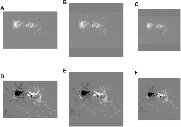
FIGURE 1. Example of the uniform magnetogram size. (A), (B), (C) are the transverse magnetograms. (A) is the original transverse magnetogram, (B) is the filled square transverse magnetogram, and (C) is the final input transverse magnetogram with the size of ×160 160 pixels. (D), (E), and (F) provide the process of the conversion for the corresponding longitudinal magnetogram.

2.3 Calculation of the total unsigned magnetic flux in the neutral line

Statistical results and forecasting experience show that most major flares are observed in the vicinity of neutral lines (Schrijver, 2007; Mason and Hoeksema, 2010; Welsch et al., 2011; Moore et al., 2012; Vasantharaju et al., 2018). Based on this fact, Schrijver (2007) introduced the quantity R, the total unsigned magnetic flux in the neutral region. This study and subsequent studies demonstrated that R is a very important parameter determining whether a flare is produced in one AR. Ji et al. (2020) trained interval-based time series classifiers for All-Clear flare forecasting by using the quantity of R and total unsigned flux. Tang et al. (2021) built a solar flare prediction model with SHARP magnetograms and magnetic parameters including the quantity of R. Here, applying the method of Schrijver (2007), we calculate the quantity R.

First, two bitmaps are generated from the magnetogram, containing a positive mapping and a negative mapping, with a positive field of 1 in the positive mapping (where B ≥ 200 G) and the rest of the pixels as 0; and a negative field of −1 in the negative mapping (where B ≤ −200 G) and the remaining pixels are 0. Then, we generate the neutral line mask by multiplying the positive and negative mappings, which are convolved using a Gaussian kernel. After that, the R value is calculated by summing the absolute values of the magnetic intensity values in the neutral region. Figure 2 gives an example of the extracted neutral line in AR 1465. a) is the longitudinal magnetic field, b) is the mask of positive field derived, c) is the mask of negative field derived, and d) is the extracted neutral region with the non-zero magnetic field values.

FIGURE 2

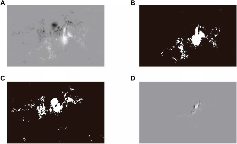
FIGURE 2. An example of the extracted neutral line in AR 1465 observed by SDO/HMI at 16:00 UT, 2012 April 25. (A) is the longitudinal magnetic field, (B) is the mask of positive field derived, (C) is the mask of negative field derived, and (D) is the extracted neutral region with the non-zero magnetic field values.

The relationship between R and solar flare productivities is analyzed. We split the range of R values into 25 equal-sized bins from its maximum to minimum, and then count the numbers of flare samples, non-flare samples, and total samples, shown in Figure 3A. Based on the numbers of flare samples and total samples in each bin, the flare productivities are calculated. Since the number of samples with R greater than 1E7 $\mathrm{G}\mathrm{s}\times {\mathrm{p}\mathrm{i}\mathrm{x}\mathrm{e}\mathrm{l}}^2$ is small, those bins greater than 1E7 $\mathrm{G}\mathrm{s}\times {\mathrm{p}\mathrm{i}\mathrm{x}\mathrm{e}\mathrm{l}}^2$ are combined into one bin. From Figure 3B, it can be seen that the flare productivity increases with the increase of R values. Based on this relationship, the R value is normalized, which is used as the deep learning model input.

FIGURE 3

FIGURE 3. Distributions of R values (A) and the corresponding flare productivities (B). X-axis is the value of R. In (A), the red, blue and green dots indicate the number of total samples, non-flare samples, and flare samples, respectively.

2.4 Labeling for flare and non-flare samples

These AR samples are labeled based on the occurrence of M-class or larger flares within the next 48 h. When an AR produced one or more M-class or larger flares in the next 48 h, the sample is a flare sample. Conversely, it is a non-flare sample when AR did not produce any of M-class or larger flare in the next 48 h. The AR flare list is provided by NOAA/SWPC. Through the above series of data selection and processing, there are 1842 flare samples and 6988 non-flare samples for complex ARs.

3 Deep learning flare prediction models for complex ARs

3.1 Processing of the imbalance dataset

The number of flare samples is much smaller than the number of non-flare samples. Faced with the imbalanced data set, machine learning models typically predict the majority of samples, which means that flare samples are more probably to be misclassified than more non-flare samples. How to deal with the imbalance dataset is an important research in the field of machine learning. A series of methods have been proposed. Among them, resampling is a widely adopted method, which consists of undersampling (removing samples from the majority class) and oversampling (adding more examples to the minority class). Which method is better in the flare forecasting is still inconclusive. Here, we use a undersampling method to randomly select 1842 samples from the 6,988 non-flare samples. In the other study, we focused on tackling with the unbalanced dataset in the flare forecasting models (Liu et al., 2023). Thus, there are 3684 samples in total. In order to further expand the sample set, we flip the AR magnetograms horizontally and vertically. In this way, the number of samples has been increased by three times, to 11,052 cases. Figure 4 shows an example of the flipping process of an AR longitudinal magnetogram.

FIGURE 4

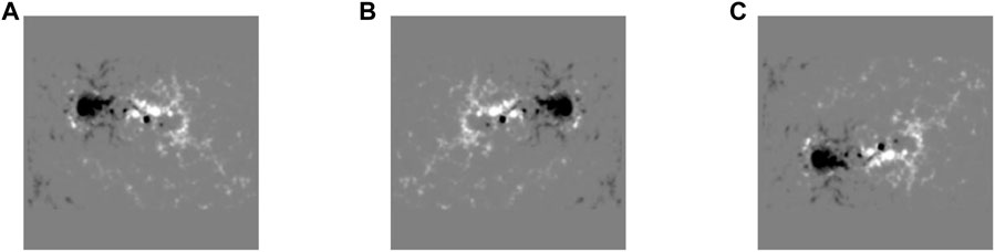
FIGURE 4. Example of flipped longitudinal magnetograms for AR 1875 observed by SDO/HMI at 08:00 UT, 2013 October 25. (A) is the AR original longitudinal magnetogram, (B) and (C) are the magnetograms after being flipped horizontally and vertically, respectively.

3.2 CNN flare forecasting models for complex ARs

CNN (Neubauer, 1998; Lecun et al., 2015; Schmidhuber, 2015) is a representative network structure in the field of deep learning. CNN can process input data with two-dimensional patterns such as images and perform well on a raw image without preprocessing. It is widely used in the computer visions such as image classification. In this study, the CNN is used to establish flare forecasting models for complex ARs. The image input of CNN generally requires a uniform size. The AR transverse and longitudinal magnetic graphs have been converted into the uniform size of ×160160 pixels.

The CNN includes two main parts. One part consists many pairs of convolutional or pooling layers, called as Feature Extraction, which separates and identifies the various features of the AR magnetic field images for analysis. Here, the convolution part contains four layers of convolution, the size of the convolution kernel is 5 × 5, and the number of kernels in the four layers are 32, 64, 128, and 256 respectively. During the convolution process all-zero padding is used with a step size of 1. The data from the convolutional layer is activated by a nonlinear activation function (Rectified Linear Unit) to improve the neural network’s ability to represent the model. The activated results are fed into the pooling layer for max pooling. During the pooling process all-zero padding is used and a kernel size of 2 × 2 with a step size of 2. The pooled data can avoid the intervention of more redundant information to prevent overfitting.

The other part is the fully connected layers, called as Classification, which utilizes the output from the previous process and predicts the flare production. The fully connected layer integrates highly abstract features after multiple convolutions and then normalizes them to output the probability of each classification case. In the fully connected layer, there is one hidden layer containing 512 neurons. The output layer has two nodes each corresponding to whether the output corresponds to an outbreak of flares or not. When an R-value is input to the model, it enters the fully connected layer along with the features extracted from the magnetogram for the classification process. The output of the fully connected neural network pass through the softmax function to obtain the probability distribution of the classification. The results are then compared with the data labels to get the cross entropy, so as to gain the loss function.

The model is optimized by the gradient descent optimizer. Before the network undergoes the optimization process, the training hyperparameters are set empirically. The batch size of the model is 100, the number of iterations is 2000, and the learning rate is 0.0005. All model hyperparameters and training hyperparameters are shown in Table 1. The corresponding loss function curve on the training sets and the accuracy curve on the test sets are shown in Figure 5, which denote that the models have learned some of the features and are in a stable state after 2000 steps.

TABLE 1

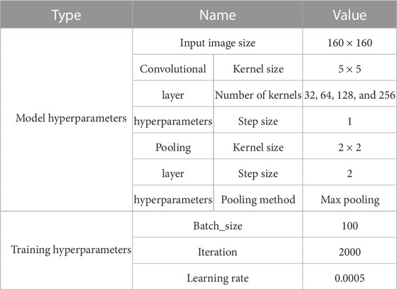
TABLE 1. CNN hyperparameter settings.

FIGURE 5

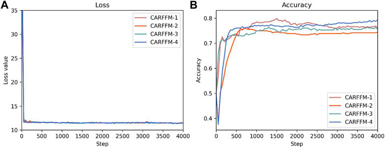
FIGURE 5. The loss function curve on the training sets (A) and the accuracy curve on the test sets (B) of the four models during the training process.

To evaluate the impact of different inputs, four models are established by using the same CNN structure and hyperparameters, which are named as Complex Active Region Flare Forecasting Model (CARFFM) -1 CARFFM-2, CARFFM-3 and CARFFM-4. In the model of CARFFM-1, the AR longitudinal magnetograms as a single channel are input into the Feature Extraction process. In the model of CARFFM-2, the AR longitudinal magnetograms and the corresponding transverse magnetograms as two channels enters the Feature Extraction process. The AR longitudinal magnetogram and the corresponding transverse magnetogram are independent of each other in this process. Based on the models of CARFFM-1 and -2, the parameter of R after being normalized is directly input into the fully connected layer in the models of CARFFM-3 and -4. These four models’ structure and inputs are shown in Figure 6 in detail.

FIGURE 6

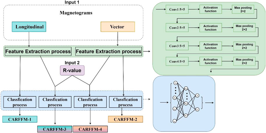
FIGURE 6. The structures of the models CARFFM −1, −2, −3, and −4.

Besides, the cross-validation technique is used. Through cross-validation, we can see the generalization ability and stability of the model. During the process of cross-validation, the original data samples are divided into several parts. The CNN model trains on all parts, except one. And the model is tested on the remaining part. The process continues until all parts are used once as test data. The average of all results is calculated to evaluate the model’s performance. Here, ten-fold cross-validation is used. The obtained complex AR flare and non-flare samples are divided into ten equal parts in time order.

It is need to explain why we divide samples in chronological order, not randomly. Dividing samples in chronological order can ensure that there are completely different active region samples in the test and training sets. Due to the relatively slow motion of photospheric magnetic field, adjacent images in the same AR are very similar, although the SHARP vector magnetograms are taken every 96 min to ensure changes between consecutive AR samples. If the samples are divided randomly, there can be similar AR samples in the test and training set, and the model will have a pseudo good performance owing to the over-fitting.

4 Model evaluation

The model evaluation is one important process in building models. The four flare forecasting model results are given by four parameters of “true positive (TP)", “true negative (TN)", “false negative (FN)" and “false positive (FP)”. TP is the number of successfully predicted flare samples and TN is the number of correctly predicted non-flare samples. FN is the number of flare samples wrongly forecasted as “non-flare” and FP is the number of non-flare samples wrongly forecasted as “flare”. The four models CARFFM -1, −2, −3 and −4 have TP of 119 ± 22, 119 ± 22, 120 ± 25, and 124 ± 18, TN of 143 ± 19, 148 ± 18, 144 ± 18, and 144 ± 22, FN of 65 ± 22, 65 ± 22, 64 ± 25, and 60 ± 18, and FP of 41 ± 19, 36 ± 18, 40 ± 18, and 40 ± 22, respectively. The values of these four parameters are shown in Table 2.

TABLE 2

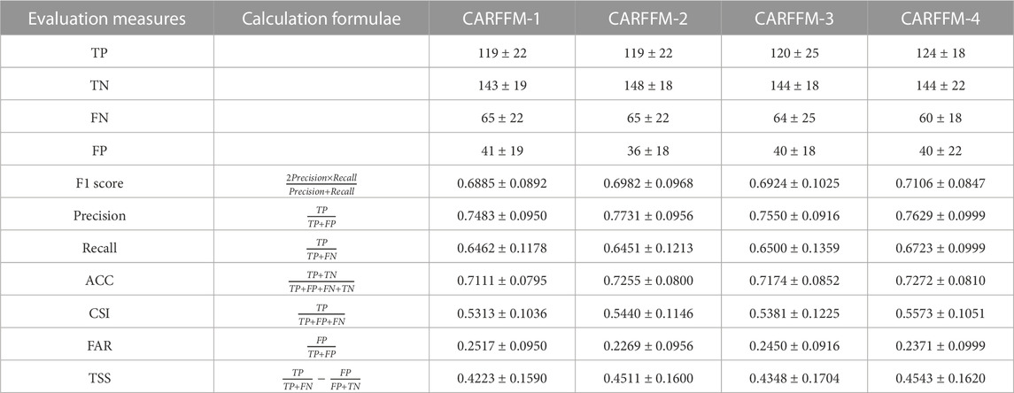
TABLE 2. Evaluation measures and values.

To further quantitatively evaluate the performance of the models, several commonly used measures are calculated: Precision, Recall, F1 score (Goutte and Gaussier, 2005), Accuracy (ACC), Critical success index (CSI) (Donaldson et al., 1975), False alarm rate (FAR), and True skill Statistics (TSS) (Hanssen and Kuipers, 1965). In operational flare forecasting, forecasters are mainly concerned with TP, FN and FP. These three parameters need to be taken into account simultaneously when evaluating the model. Therefore, we choose F1 score as the main evaluation index, and ACC, CSI, and TSS are as references. The F1 score is the harmonic average of Precision and Recall, which includes TP, FN, and FP at the same time. ACC measures the total correct forecasting rate. CSI is the ratio of TP to the sum of TP, FP, and FN. TSS is the difference between the ratio of the correctly predicted flare samples to the total flare samples and the ratio of the incorrectly forecasted flare samples to the total non-flare samples. The higher this value is, the better the model performance is. The measure equations and the corresponding mean values and standard deviations for the four models are shown in Table 2. In the ten-fold cross validation, the large mean value and small standard deviation of the measures (F1 score, ACC, CSI, and TSS) means that the model has a better performance for most of the test parts.

Here, the mean values and the standard deviations of F1 score for CARFFM-1, CARFFM-2, CARFFM-3, and CARFFM-4 are 0.6885 ± 0.0892, 0.6982 ± 0.0968, 0.6924 ± 0.1025, and 0.7106 ± 0.0847, respectively. That is, CARFFM-4 has the largest mean value of F1 score, while CARFFM-1 does the smallest mean value of F1 score. It is denoted that CARFFM-4 has the best performance, CARFFM-2 and CARFFM-3 have better performance, CARFFM-1 has the relatively poor performance, although the difference in the model performance is not big. The evaluation scores of ACC, CSI and TSS give the same conclusion, such as TSS, which scores of the four models are 0.4223 ± 0.1590, 0.4511 ± 0.1600, 0.4348 ± 0.1704, and 0.4543 ± 0.1620, respectively.

The difference in model performance comes from the different inputs. In the model of CARFFM-4, there are 3 types of inputs including the AR longitudinal magnetogram, transverse magnetogram and the parameter of R, while only AR longitudinal magnetogram is used in the model of CARFFM-1. In the models of CARFFM-2 and CARFFM-3, there are two types of inputs. Therefore, it is got that more valuable inputs can improve the model forecasting performance.

5 Summary and conclusion

Solar flares are important space weather events, which are mainly produced in ARs, especially in complex ARs. Many studies have been carried out on the establishment of flare prediction models for all ARs. But so far, few studies have been carried on establishing flare forecasting models for complex ARs.

By using the SDO/HMI SHARP magnetic field data from 1 May 2010 to 31 December 2018, four flare forecasting CNN models are established for complex ARs, called as CARFFM −1, −2, −3 and −4. In the model of CARFFM-1, only AR longitudinal magnetograms are used as input for Feature Extraction in the CNN structure. In the model of CARFFM-2, AR vector magnetograms containing the intensity of the longitudinal and transverse components are used as input for Feature Extraction. Based on the models of CARFFM-1 and CARFFM-2, the normalized physical quantity of R in the neutral line is input to Classification, or the fully connected layer, in the models of CARFFM -3 and −4. These four models can provide the forecasting result for the occurrence of M-class or above flares in the complex ARs for the next 48 h.

To compare the forecasting performance of the four models, many evaluation measures are calculated. F1 score are chosen as the main measure, and ACC, CSI, and TSS are as references. The mean values of F1 score for the four models of CARFFM −1, −2, −3 and −4 are 0.6885, 0.6982, 0.6924, and 0.7106, respectively. It is shown that the CARFFM-4 has the biggest mean value of F1 score, and the CARFFM-2 and the CARFFM-3 have moderate mean values of F1 score, and in the model of CARFFM-1, the mean value of F1 score is the smallest. Other evaluation metrics also show the same results, such as TSS. The TSS of the four models are 0.4223 ± 0.1590, 0.4511 ± 0.1600, 0.4348 ± 0.1704, and 0.4543 ± 0.1620, respectively. As a whole, the CARFFM-4 has the best prediction performance, and the prediction performance of the CARFFM-1 is relatively poor. Therefore, we consider that more valuable inputs are beneficial to improve the model forecasting performance.

In this study, we have established flare forecasting models for complex ARs. However, in order to further improve the operational flare forecasting performance, there are still a lot of work to do. First, the flare forecasting models should consider AR evolution or motion information before the flare eruption, which is important to determine the occurrence of flares. Second, more magnetic parameters can be used, such as current helicity and free energy density, which have physical meanings and play an effective role. And last but not least, how to better utilize the AR vector magnetic map information is an important open question. Here, the longitudinal and transverse strength information of complex ARs is considered merely, the directional information of transverse fields is not included.

Data availability statement

The original contributions presented in the study are included in the article/supplementary material, further inquiries can be directed to the corresponding author.

Author contributions

ML, YC, BL, JW, and XW meet the authorship criteria, and agree to be accountable for the content of the work. All authors contributed to the article and approved the submitted version.

Funding

This work is supported by the National Science Foundation of China (Grant No.42074224), the Key Research Program of the Chinese Academy of Sciences (Grant No. ZDRE-KT-2021-3) and Pandeng Program of National Space Science Center, Chinese Academy of Sciences.

Acknowledgments

We acknowledge the SDO/HMI team members for providing SDO/HMI magnetograms (http://jsoc.stanford.edu/) and the NOAA/SWPC team members for providing the solar flare list and active region description.

Conflict of interest

The authors declare that the research was conducted in the absence of any commercial or financial relationships that could be construed as a potential conflict of interest.

Publisher’s note

All claims expressed in this article are solely those of the authors and do not necessarily represent those of their affiliated organizations, or those of the publisher, the editors and the reviewers. Any product that may be evaluated in this article, or claim that may be made by its manufacturer, is not guaranteed or endorsed by the publisher.

References

Ataç, T. (1987). Statistical relationship between sunspots and major flares. Astrophysics Space Sci.129, 203–208. doi:10.1007/bf00717871

CrossRef Full Text | Google Scholar

Benvenuto, F., Piana, M., Campi, C., and Massone, A. M. (2017). A hybrid supervised/unsupervised machine learning approach to solar flare prediction. Astrophysical J.853, 90. doi:10.3847/1538-4357/aaa23c

CrossRef Full Text | Google Scholar

Bobra, M. G., and Couvidat, S. (2015). Solar flare prediction using SDO/HMI vector magnetic field data with a machine-learning algorithm. Astrophysical J.798, 135. doi:10.1088/0004-637x/798/2/135

CrossRef Full Text | Google Scholar

Bobra, M. G., Sun, X., Hoeksema, J. T., Turmon, M., Liu, Y., Hayashi, K., et al. (2014). The helioseismic and magnetic imager (HMI) vector magnetic field pipeline: Sharps -- space-weather HMI active region patches. Sol. Phys.289, 3549–3578. doi:10.1007/s11207-014-0529-3

CrossRef Full Text | Google Scholar

Chen, A., Wang, J., Li, J., Feynman, J., and Zhang, J. (2011). Statistical properties of superactive regions during solar cycles 19-23. Astronomy Astrophysics534, A47. doi:10.1051/0004-6361/201116790

CrossRef Full Text | Google Scholar

Chen, A., Ye, Q., and Wang, J. (2021). Flare index prediction with machine learning algorithms. Sol. Phys.296, 150. doi:10.1007/s11207-021-01895-1

CrossRef Full Text | Google Scholar

Chen, J., Li, W., Li, S., Chen, H., Zhao, X., Peng, J., et al. (2022). Benefit of uracil-tegafur used as a postoperative adjuvant chemotherapy for stage IIA colon cancer. Space Sci. Technol.2022, 10. doi:10.3390/medicina59010010

CrossRef Full Text | Google Scholar

Cicogna, D., Berrilli, F., Calchetti, D., Moro, D. D., Giovannelli, L., Benvenuto, F., et al. (2021). Flare forecasting algorithms based on high-gradient polarity inversion lines in active regions. Astrophysical J.915, 38. doi:10.3847/1538-4357/abfafb

CrossRef Full Text | Google Scholar

Cui, Y., Rong, L., Zhang, L., He, Y., and Wang, H. (2007). Correlation between solar flare productivity and photospheric magnetic field properties: 1. Maximum horizontal gradient, length of neutral line, number of singular points. Sol. Phys.237, 45–59. doi:10.1007/s11207-006-0077-6

CrossRef Full Text | Google Scholar

Deshmukh, V., Flyer, N., van der Sande, K., and Berger, T. (2022). Decreasing false-alarm rates in CNN-based solar flare prediction using SDO/HMI data. Astrophysical J. Suppl. Ser.260, 9. doi:10.3847/1538-4365/ac5b0c

CrossRef Full Text | Google Scholar

Donaldson, R. J., Dyer, R. M., and Kraus, M. J. (1975). An objective evaluator of techniques for predicting severe weather events. American Meteorological Society.

Google Scholar

Eren, S., Kilcik, A., Atay, T., Miteva, R., Yurchyshyn, V., Rozelot, J. P., et al. (2017). Flare-production potential associated with different sunspot groups. Mon. Notices R. Astronomical Soc.465, 68–75. doi:10.1093/mnras/stw2742

CrossRef Full Text | Google Scholar

Georgoulis, M. K. (2018). The ambivalent role of field-aligned electric currents in the solar atmosphere.

Google Scholar

Georgoulis, M. K., Titov, V. S., and Mikić, Z. (2012). Non-neutralized electric current patterns in solar active regions: Origin of the shear-generating lorentz force. Astrophysical J.761, 61. doi:10.1088/0004-637x/761/1/61

CrossRef Full Text | Google Scholar

Goutte, C., and Gaussier, E. (2005). A probabilistic interpretation of precision, Recall and F-score, with implications for evaluation. Springer Berlin Heidelberg.

Google Scholar

Guastavino, S., Marchetti, F., Benvenuto, F., Campi, C., and Piana, M. (2022). Implementation paradigm for supervised flare forecasting studies: A deep learning application with video data. Astronomy Astrophysics662, A105. doi:10.1051/0004-6361/202243617

CrossRef Full Text | Google Scholar

Guastavino, S., Marchetti, F., Benvenuto, F., Campi, C., and Piana, M. (2023). Operational solar flare forecasting via video-based deep learning. Front. Astronomy Space Sci.9. doi:10.3389/fspas.2022.1039805

CrossRef Full Text | Google Scholar

Guerra, J. A., Pulkkinen, A., and Uritsky, V. M. (2015). Ensemble forecasting of major solar flares: First results. Space weather.13, 626–642. doi:10.1002/2015sw001195

CrossRef Full Text | Google Scholar

Hanssen, A. W., and Kuipers, W. J. A. (1965). On the relationship between the frequency of rain and various meteorological parameters. Meded. Verh.81, 2.

Google Scholar

Harrison, R. A. (1995). The nature of solar flares associated with coronal mass ejection. Astron. Astrophys.304, 585.

Google Scholar

Huang, X., Wang, H., Xu, L., Liu, J., Li, R., and Dai, X. (2018). Deep learning based solar flare forecasting model. I. results for line-of-sight magnetograms. Astrophysical J.856, 7. doi:10.3847/1538-4357/aaae00

CrossRef Full Text | Google Scholar

Ji, A., Aydin, B., Georgoulis, M. K., and Angryk, R. (2020). “All-clear flare prediction using interval-based time series classifiers,” in 2020 IEEE international conference on big data (big data), 4218–4225. doi:10.1109/BigData50022.2020.9377906

CrossRef Full Text | Google Scholar

Jonas, E., Bobra, M., Shankar, V., Todd Hoeksema, J., and Recht, B. (2018). Flare prediction using photospheric and coronal image data. Sol. Phys.293, 48. doi:10.1007/s11207-018-1258-9

CrossRef Full Text | Google Scholar

Kahler, S. W. (1992). Solar flares and coronal mass ejections. Annu. Rev. Astronomy Astrophysics30, 113–141. doi:10.1146/annurev.aa.30.090192.000553

CrossRef Full Text | Google Scholar

Knipp, D. J. (2005). Understanding space weather and the Physics behind it: A textbook for undergraduates. American Geophysical Union, Spring Meeting.

Google Scholar

Lecun, Y., Bengio, Y., and Hinton, G. (2015). Deep learning. Nature521, 436–444. doi:10.1038/nature14539

PubMed Abstract | CrossRef Full Text | Google Scholar

Lee, K., Moon, Y. J., Lee, J. Y., Lee, K. S., and Na, H. (2012). Solar flare occurrence rate and probability in terms of the sunspot classification supplemented with sunspot area and its changes. Sol. Phys.281, 639–650. doi:10.1007/s11207-012-0091-9

CrossRef Full Text | Google Scholar

Li, M., Cui, Y., Luo, B., Ao, X., Liu, S., Wang, J., et al. (2022). Knowledge-informed deep neural networks for solar flare forecasting. Space weather.20, e2021SW002985.

CrossRef Full Text | Google Scholar

Liu, H., Liu, C., Wang, J., and Wang, H. (2019). Predicting solar flares using a long short-term memory network. Astrophysical J.877, 121. doi:10.3847/1538-4357/ab1b3c

CrossRef Full Text | Google Scholar

Liu, S., Wang, J., Li, M., Cui, Y., Shi, Y., Luo, B., et al. (2023). A selective up-sampling method applied upon unbalanced data for flare prediction: potential to improve model performance. Front. Astron. Space Sci.10, 1082694. doi:10.3389/fspas.2023.1082694

CrossRef Full Text | Google Scholar

Liu, Y., Sun, X., TöRöK, T., Titov, V. S., and Leake, J. E. (2017). Electric-current neutralization, magnetic shear, and eruptive activity in solar active regions. Astrophysical J. Lett.846, L6. doi:10.3847/2041-8213/aa861e

CrossRef Full Text | Google Scholar

Mason, J. P., and Hoeksema, J. T. (2010). Testing automated solar flare forecasting with 13 Years of michelson Doppler imager magnetograms. Astrophysical J.723, 634–640. doi:10.1088/0004-637x/723/1/634

CrossRef Full Text | Google Scholar

Moore, R. L., Falconer, D. A., and Sterling, A. C. (2012). The limit of magnetic-shear energy in solar active regions. Astrophysical J.750, 24. doi:10.1088/0004-637x/750/1/24

CrossRef Full Text | Google Scholar

Neubauer, C. (1998). Evaluation of convolutional neural networks for visual recognition. IEEE Trans. Neural Netw.9, 685–696. doi:10.1109/72.701181

PubMed Abstract | CrossRef Full Text | Google Scholar

Nishizuka, N., Sugiura, K., Kubo, Y., Den, M., and Ishii, M. (2018). Deep Flare Net (DeFN) model for solar flare prediction. Astrophysical J.858, 113. doi:10.3847/1538-4357/aab9a7

CrossRef Full Text | Google Scholar

Nishizuka, N., Sugiura, K., Kubo, Y., Den, M., Watari, S., and Ishii, M. (2017). Solar flare prediction model with three machine-learning algorithms using ultraviolet brightening and vector magnetograms. Astrophysical J.835, 156. doi:10.3847/1538-4357/835/2/156

CrossRef Full Text | Google Scholar

Pesnell, W. D., Chamberlin, B., and Chamberlin, P. C. (2012). The solar dynamics observatory (SDO). Sol. Phys.275, 3–15. doi:10.1007/s11207-011-9841-3

CrossRef Full Text | Google Scholar

Raboonik, A., Safari, H., Alipour, N., and Wheatland, M. S. (2016). Prediction of solar flares using unique signatures of magnetic field images. Astrophysical J.834, 11. doi:10.3847/1538-4357/834/1/11

CrossRef Full Text | Google Scholar

Sammis, I., Tang, F., and Zirin, H. (2000). The dependence of large flare occurrence on the magnetic structure of sunspots. Astrophysical J.540, 583–587. doi:10.1086/309303

CrossRef Full Text | Google Scholar

Scherrer, P. H., Schou, J., Bush, R. I., Kosovichev, A. G., Bogart, R. S., Hoeksema, J. T., et al. (2012). The helioseismic and magnetic imager (HMI) investigation for the solar dynamics observatory (SDO). Sol. Phys.275, 207–227. doi:10.1007/s11207-011-9834-2

CrossRef Full Text | Google Scholar

Schmidhuber, J. (2015). Deep learning in neural networks: An overview. Neural Netw.61, 85–117. doi:10.1016/j.neunet.2014.09.003

PubMed Abstract | CrossRef Full Text | Google Scholar

Schrijver, C. J. (2007). A characteristic magnetic field pattern associated with all major solar flares and its use in flare forecasting. Astrophysical J.655, L117–L120. doi:10.1086/511857

CrossRef Full Text | Google Scholar

Sun, H., Ward, I. V., and Chen, Y. (2021). Improved and interpretable solar flare predictions with spatial & topological features of the polarity-inversion-line masked magnetograms. Space weather.19, e2021SW002837.

CrossRef Full Text | Google Scholar

Sun, Z., Bobra, M. G., Wang, X., Wang, Y., Sun, H., Gombosi, T., et al. (2022). Predicting solar flares using CNN and LSTM on two solar cycles of active region data. Astrophysical J.931, 163. doi:10.3847/1538-4357/ac64a6

CrossRef Full Text | Google Scholar

Tang, R., Liao, W., Chen, Z., Zeng, X., Wang, J.-S., Luo, B., et al. (2021). Solar flare prediction based on the fusion of multiple deep-learning models. Astrophysical J. Suppl. Ser.257, 50. doi:10.3847/1538-4365/ac249e

CrossRef Full Text | Google Scholar

TöRöK, T., Leake, J. E., Titov, V. S., Archontis, V., Mikić, Z., Linton, M. G., et al. (2014). Distribution of electric currents in solar active regions. Astrophysical J. Lett.782, L10. doi:10.1088/2041-8205/782/1/l10

CrossRef Full Text | Google Scholar

Vasantharaju, N., Vemareddy, P., Ravindra, B., and Doddamani, V. H. (2018). Statistical study of magnetic nonpotential measures in confined and eruptive flares. Astrophysical J.860, 58. doi:10.3847/1538-4357/aac272

CrossRef Full Text | Google Scholar

Wang, H. N., Cui, Y. M., Li, R., Zhang, L. Y., and Han, H. (2008). Solar flare forecasting model supported with artificial neural network techniques. Adv. Space Res.42, 1464–1468. doi:10.1016/j.asr.2007.06.070

CrossRef Full Text | Google Scholar

Wang, J., Zhang, Y., Webber, S. A. H., Liu, S., Meng, X., and Wang, T. (2020). Solar flare predictive features derived from polarity inversion line masks in active regions using an unsupervised machine learning algorithm. Algorithm Astrophysical J.892, 140. doi:10.3847/1538-4357/ab7b6c

CrossRef Full Text | Google Scholar

Welsch, B. T., Christe, S., and Mctiernan, J. M. (2011). Photospheric magnetic evolution in the WHI active regions. Sol. Phys.274, 131–157. doi:10.1007/s11207-011-9759-9

CrossRef Full Text | Google Scholar

Yashiro, S., and Gopalswamy, N. (2009). “Statistical relationship between solar flares and coronal mass ejections,” in Universal heliophysical processes. Editors N. GOPALSWAMY, and D. F. WEBBMarch 01 2009 233.

Google Scholar

Yuan, Y., Shih, F. Y., Ju, J., and Wang, H. M. (2010). Automated flare forecasting using a statistical learning technique. Res. Astronomy Astrophysics10, 785–796. doi:10.1088/1674-4527/10/8/008

CrossRef Full Text | Google Scholar