Estimating intermittency significance by means of surrogate data: implications for solar wind turbulence

1 Introduction

Isotropy and scale invariance (self-similarity) are two fundamental hypotheses of Kolmogorov’s (1941) hydrodynamic turbulence theory. Tu and Marsch (1993), Bruno et al. (2003), Bruno and Bavassano (1991), Bavassano and Bruno (1992), and Tu and Marsch (1990) demonstrated that solar wind turbulent fluctuations are not isotropic or scale-invariant (see also, Frisch, 1995). This fact challenges the hypothesis of self-similarity and a constant and uniform energy transfer rate from large to small eddies, i.e., the key elements of turbulence as illustrated by Richardson’s (1920) energy cascade (Obukhov, 1962; Landau and Lifshitz, 1971; Bruno, 2019). The irregularity and fragmentation of the turbulence topology are known as intermittency (Frisch, 1995). The effect of intermittency is detected as a deviation from self-similarity of fluctuations at different scales; i.e., the global scale invariance assumed by Kolmogorov remains valid only locally, in limited regions of space, rendering multifractal approaches more suited as investigation tools (Frisch, 1995; Wawrzaszek and Echim, 2021). By comparing experimental results with several energy cascade models, Meneveau and Sreenivasan (1991) argued that the multifractal (intermittent) distribution of the rate of turbulent energy dissipation indicates that turbulent flows can be described as self-similar multiplicative fragmentation processes. As such, intermittency is revealed by the increasing departure from a Gaussian of the probability distribution function (PDF) of the fluctuations of a variable at smaller and smaller scales (Sorriso-Valvo et al., 1999; Bruno et al., 2004). In other words, extreme events occur with higher probabilities than predicted by the normal distribution. Thus, second-order moment analysis, such as spectral analysis, no longer provides a full description of turbulence statistics. Biskamp (1993) and Frisch (1995) demonstrated that intermittent fluctuations can be characterized by higher-order moments of the PDFs, the structure functions (SFs), where the nonlinear trend of the SF exponents is a manifestation of intermittency.

Burlaga (1991) demonstrated the universal character of intermittency from in situ solar wind data through the remarkable similarity at scales of millions of kilometers and meters, the latter of which was observed in laboratory experiments (Anselmet et al., 1984). The author pointed toward a mixture of sheets and space-filling eddies within turbulent media. Using Helios 2 data, Bruno et al. (2003) investigated the radial evolution of intermittency in the inner heliosphere between 0.3 and 0.9 astronomical units (AU) from the Sun. Yordanova et al. (2009) analyzed solar wind turbulence and intermittency using Ulysses data (Balogh et al., 1992) and determined how intermittency properties vary with heliospheric latitudes, distances from the Sun, or solar activity for both slow and fast solar wind.

A classical intermittency descriptor, the flatness, denoted in the following by κ, is defined as a normalized fourth-order moment of the PDF:

$\kappa =\frac{{SF}_4}{{SF}_2^2},(1)$

where ${SF}_q=〈{\left|\delta X\left(\tau \right)\right|}^q〉$ is the q^th-order moment of the PDF, $〈\dots 〉$ denotes averaging, and δX is an ensemble of fluctuations at time scale τ, determined from differencing the original signal for different values of τ:

$\delta X=X\left(t+\tau \right)-X\left(t\right).(2)$

It should be noted that the ensemble δX is built by moving the window of length τ over the entire signal. In general, two successive positions of the window overlap by several points, n₀. According to Frisch (1995), the continuous growth of κ at smaller scales is a characteristic of intermittency. Because the flatness of a Gaussian distribution of fluctuations (κ = 3) is well specified, deviations in the flatness can be used to characterize the nature of intermittent fluctuations. If κ grows faster, then the signal is considered more intermittent; if κ remains constant for some considered scales, those scales are self-similar and not intermittent; and $\kappa \ne 3$ signals non-Gaussian statistics (Bruno et al., 2003).

The evaluation of κ, together with a multifractal description, can be seen as a class of methods that provide a quantitative estimation of intermittency. Qualitatively, intermittency is assessed based on the anomalous scaling of SF or from the wavelet analysis of the signal and estimation of the local intermittency measure (Wawrzaszek and Echim, 2021 for a recent review).

Higher-resolution observations and simulations of space plasma turbulence suggest a decrease or saturation of the intermittency for scales at the boundary between inertial and kinetic range, in contrast with previous studies suggesting a continuous increase of the intermittency below proton scales (Alexandrova et al., 2008) or the expected return to Gaussianity at these scales, which should arise in incoherent wave interactions that mix and randomize the phases. For example, an analysis of Cluster and Advanced Composition Explorer (ACE) data in the shocked and unshocked near-Earth solar wind suggests that intermittency originates from phase synchronization resulting from nonlinear multiscale interactions of large-amplitude coherent structures (Chian and Miranda, 2009). This study uses the phase coherence technique based on surrogate data to determine the phase coherence (PC) index (Koga et al., 2007 and references therein). Through the PC index, the original data were compared with two sets of surrogates with identical power spectra, whose phase spectra are either completely random (PC = 0) or fully correlated (PC = 1). Chian and Miranda (2009) demonstrated the constant growth of the PC index through the inertial range, from large to small scales, and following the same behavior as κ up to a maximum value. The authors showed that the peak observed in the curves of both κ and PC occurs at time scales corresponding to the spectral breakpoint between the inertial and kinetic ranges. They argued that, below this point, both κ and PC start decreasing as interactions between waves and particles become dominant and act to decrease phase synchronization.

Wan et al. (2012a) or Wu et al. (2013), using ACE and Cluster data in the solar wind at one AU and spectral or particle-in-cell (2D-PIC) simulations, observed the increase in kurtosis at proton scales, which signals the presence of coherent structures at these scales, but they also noted that the growth of kurtosis is reduced, most probably due to physical phenomena at kinetic scales. They suggest that the decrease in kurtosis (or κ-3) involves some incoherent dynamics due to waves or other phase-randomizing structures. Through a multipoint analysis of Cluster data, Yordanova et al. (2015) also hinted toward saturation of the kurtosis, i.e., scale invariance or mono-fractality, of the sub-proton fluctuations. Through kinetic simulations, Wan et al. (2012b) or Karimabadi et al. (2013) found that heating and dissipation are highly non-uniform in astrophysical and space plasmas and that the strong cascade observed at sub-proton scales is due to coherent current sheets, i.e., the most intermittent structures, as argued by Veltri (1999) and Veltri and Mangeney (1999). They concluded that a mixture of coherent structures, in the form of current sheets and waves, is the source of intermittent plasma turbulence. Similar ideas were suggested by Chang (2015), who considered intermittency as a manifestation of space plasma complexity.

In an interesting study, Borovsky and Podesta (2015) showed that the thickness of current sheets affects the power spectral density (PSD) of the solar wind magnetic field. Through a technique of time stretching of the original data and comparison with artificially generated data, they demonstrate that, as the current sheet thickness increases, the frequency break between inertial and kinetic ranges is shifted toward smaller values (as per Chen et al., 2014) and the Fourier power at the breakpoint decreases.

Using Parker Solar Probe (PSP; Fox et al., 2016) observations of the young solar wind, unaffected by foreshock or instrumental noise (as might be the case with near-Earth observations at 1 AU), Chibber et al. (2021) demonstrated that sub-proton scales remain intermittent close to the Sun, at ∼0.17 AU, by establishing that the kurtosis does not re-Gaussianize at sub-ion scales but remains approximately constant between 10 and 0.1 d_i, where d_i is the ion inertial length.

Roberts et al. (2022) investigated both time and space magnetic field increments using 12 years of Cluster observations to assess the intermittency properties of solar wind plasma. A maximum of kurtosis is reported at ion scales, and only weak non-Gaussian fluctuations are reported at sub-ion scales. For the compressive component, the authors demonstrated its spatial anisotropy, evidenced by the differences observed between temporal and spatial increments measured perpendicular to the flow, and observed a higher variability of κ behavior, either increasing throughout both the inertial and sub-ion scales or displaying a maximum at larger, inertial range scales associated with magnetic holes. In another statistical study of more than 3000-time series measured by the PSP and Solar Orbiter (Müller et al., 2020) in the solar wind, Sioulas et al. (2022) also observed a maximum of the kurtosis that seems to display a shift toward smaller scales as the distance from the Sun increases.

The data analyzed in this study show high variability in the magnetic intermittency of the young solar wind probed by the PSP during its first encounter (E1). The data span a relatively narrow time interval, 01–09 November 2018, during which the PSP travels between approximately [0.17,0.22] AU from the Sun. In this study, we disentangle the sources of the intermittency by comparing the PSP observations with artificially generated data, i.e., surrogates (Theiler et al., 1992), that are consistent with a null hypothesis that we aim to invalidate and that may indicate the nature of the nonlinearity of the signal. The paper is structured as follows. In Section 2, we describe the analyzed data; in Section 3 and Section 4, we describe the methodology, introduce some other premises for the analysis, and describe the results of our study; and in Section 5, we summarize the conclusions.

2 Data

We analyzed magnetic field data provided by the PSP during the probe’s first perihelion, 01–09 November 2018, further referred to as Sig1. During this time interval, the PSP measured the solar wind at a distance of ∼0.17 AU from the Sun. The outboard fluxgate magnetometer (MAG) of the FIELDS instrument suite (Bale et al., 2016) provided magnetic field data, B, at a cadence of up to 293 Hz. We focused on the behavior of magnetic energy density fluctuations, B². B² was naturally chosen as a proxy for the magnetic energy, and the analysis of its fluctuations was relevant in the context of intermittent turbulence as we also discussed the turbulent energy transfer between scales. Magnetic field data during the first 3 days of the analyzed time interval were recorded at lower cadences, e.g., 146 or 73 Hz; consequently, we down-sampled the entire data set to the lowest resolution of the data, i.e., averaged to 73 Hz. In Figure 1, the time series of B² is shown in the upper panel, and the time series of the proton velocity data from the Solar Probe Cup (SPC) on the SWEAP instrument suite (Kasper et al., 2016; Case et al., 2020) is shown in the middle panel. The plasma bulk velocity distribution is indicative of a steady state of slow solar wind, with V < 500 km s⁻¹ for most of the considered time interval, except for the last day, 9 November 2018, when the PSP may have passed over a small coronal hole and sampled relatively fast wind above 600 km s⁻¹ (Chhiber et al., 2020). This interval was analyzed in numerous studies and determined to be highly intermittent with various types of intermittent structures (Astrophysical Journal Supplement Series, 246, Volume 2). For example, Bale et al. (2019) or Horbury et al. (2020) evidenced the presence of switchbacks or jets in the magnetic and velocity fields; Dudok de Wit et al. (2020) examined their statistics through waiting time analysis, Chhiber et al. (2020) provided an estimation of intermittent features based on partial variance increment (PVI) analysis. Bandyopadhyay et al. (2020) and Qudsi et al. (2020) examined the relation between intermittent magnetic structures and other measured quantities (energetic particle fluxes or high proton temperatures), also through waiting times and PVI, respectively.

FIGURE 1

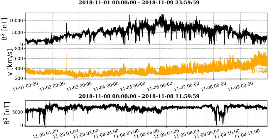
FIGURE 1. Upper and middle panels: Temporal profiles of B² and v fields during the first PSP encounter, 01–09 November 2018 (Sig1). Lower panel: A sub-sample of Sig1 recorded on 8 November 2018, between 00:00–12:00 (further referred to as Sig2).

In this paper, we discussed the intermittency of Sig1 and a chosen sub-sample of this data: the solar wind magnetic field measured on 8 November 2018, in the time interval 00:00–12:00 UT, further referred to as Sig2. The temporal profile of Sig2 is shown in Figure 1, lower panel.

3 On the nature of the nonlinearity responsible for the observed intermittency

3.1 Quantification of intermittency and premises for the analysis

We considered an argument by Hnat et al. (2005), who argued that analyses based on differencing of the original time series and the parameters derived from the overlapping differences are inevitably affected by temporal correlation. The solution to avoid such effects would be to consider non-overlapping differences, but this alternative is most often not feasible due to many factors, e.g., the limited time span of the data, as is the case with magnetosheath plasmas, time intervals that are not stationary for a sufficiently long time, and gaps in the data. To the best of our knowledge, the majority of the published papers on intermittency based on the analysis of flatness are based on overlapping differencing (like in the review by Echim et al., 2021).

Thus, we directly compared the intermittency of the slow solar wind magnetic field through κ estimated by both approaches, overlapping versus non-overlapping increments, up to scales of 100 s. Under Taylor’s (1938) hypothesis, which has been shown to be marginally satisfied for this interval (Chen et al., 2020; Duan et al., 2020; Parashar et al., 2020), temporal structures can be converted to spatial structures; hence, at a mean proton velocity of 350 km s^-1, scales of 100 s translated to spatial dimensions of 35000 km. While still small compared to the autocorrelation scales, this range of scales covered the small-scale region of the inertial range.

We also took into account a discussion by Wang et al. (2020) who demonstrated that to capture the spectral characteristics of turbulence at sub-ion scales, the use of multipoint (>2) structure functions is preferred. We tested Wang et al.’s (2020) argument on a simulated signal with prescribed spectral characteristics and found that, indeed, at the smallest (kinetic) scales, two-point SF scaling was flatter than expected while five-point SF gave more accurate results (Teodorescu et al., 2021). Consequently, in this study, we examined κ from overlapping increments computed from (a) two data points and (b) five data points defined as follows:

a) Two-point increments, [δX(τ)]:

$\delta X\left(t,\tau \right)=X\left(t+\tau \right)-X\left(t\right).(3)$

b) Five-point increments (Wang et al., 2020):

$\mathrm{\delta }X\left(t,\tau \right)=\frac{\left[X\left(t-2\tau \right)-4X\left(t-\tau \right)+6X\left(t\right)-4X\left(t+\tau \right)+X\left(t+2\tau \right)\right]}{\sqrt{35}}.(4)$

As previously mentioned, we also evaluated κ from non-overlapping increments in order to ascertain the effect of temporal correlations introduced by the classical overlapping procedure on the estimation of κ (Hnat et al., 2005):

c) non-overlapping two-point increments:

$\delta X\left(t,\tau \right)=X\left(t+\left(N+1\right)\tau \right)-X\left(t+N\tau \right).(5)$

In the third approach (as per Eq. 5), the number of samples used in the computation of the structure functions was drastically reduced. Thus, a relatively long time interval was required to access larger time scales. Even though we analyzed high-resolution PSP magnetic field measurements recorded over 9 days, the largest scale accessible that still preserves a meaningful number of increments (at least 4000) was 100 s. To retain a higher statistic of increments for the estimation of the structure functions and to access larger time scales, we focused our computations on two-point, non-overlapping increments.

3.2 Formulation of the null hypothesis

A common practice in statistical analysis involves the division of data into sub-intervals of some chosen length. The PSP data included in Sig1 were divided into four sets, each set comprising contiguous sub-intervals of fixed length. The length of sub-intervals for the four sets was defined as follows: 24 hours (set 1), 12 hours (set 2), 6 hours (set 3), and 3 hours (set 4). For each set, we computed κ and illustrated its scale dependence and time evolution in a two-dimensional (2D) graphical scalogram-like representation, as represented in Figure 2. κ computed from five-point increments is shown. The upper row of these “flatogram” 2D plots shows κ computed for sets 1 and 2, respectively. On the lower row, we showed κ for sets 3 and 4, respectively. The X-axis indicates the sub-interval number of each set, starting from 0, which is also delimited by the vertical dashed red lines in the time series of B². For example, in Figure 2A, the fifth column shows κ computed for 1 day of magnetic field measurements collected on 6 November 2018, during the PSP’s first encounter, which took place at around 03:27 UT and 0.17 AU. The Y-axis indicates the time lag of the increments in seconds, i.e., the temporal scale of the fluctuations, which, under Taylor’s hypothesis, can be transformed into a spatial scale. The minimum accessible scale is determined by the resolution of the data: at a sample rate of 73 Hz, the smallest accessible scale is around 0.03 s, while the maximum accessible scale depends on the data sample length; with 24 h data samples, the largest accessible scale is around 2 hours, while for 3 h samples, the largest scale is less than 15 minutes.

FIGURE 2

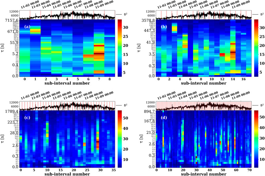
FIGURE 2. Variability of intermittency quantified by flatness, κ, when the data are divided into contiguous samples of various time lengths: (A) Set 1, 24 h sub-intervals, (B) Set 2, 12 h sub-intervals, (C) Set 3, 6 h sub-intervals, and (D) Set 4, 3 h sub-intervals. κ computed from five-point increments is shown.

All representations in Figure 2 seem to indicate high variability in the intermittency of the slow solar wind, quantified through the flatness parameter. It could be concluded that the observed pattern is suggestive of time intervals characterized by low intermittency that change with time intervals that display high intermittency levels. Moreover, it seems that when subdividing the data into smaller samples, the intermittent samples become sparser but show increased levels of intermittency.

Another recurrent feature in almost all analyzed time intervals, which is also independent of the length of the sub-intervals, is that κ reaches a maximum at scales between [1-10] s. This peculiar behavior was reported in several previous works (Chian and Miranda, 2009; Wan et al., 2012a; Wu et al., 2013; Yordanova et al., 2015; Chiber et al., 2021; Roberts et al., 2022; Sioulas et al., 2022). In Figure 2, for most data samples, the flatness grows from κ = 3 (characteristic for Gaussian processes) at large injection-range scales of the order of hundreds of seconds toward higher values for scales of the order of several seconds that still pertain to the inertial range. This behavior is considered a hallmark of intermittency. Then, κ reaches a maximum, in some cases like a peak value, in others more like a plateau distributed over 1 decade of scales in the interval [1-10] s. For smaller scales, in the kinetic range, κ starts decreasing; its value at scales below 0.1–0.5 s is close to 3. A second peak in the distribution of κ is also observed at the smallest scales for many of the sub-intervals of the four sets.

To better illustrate this point, in Figure 3 we show the classical representation of the scale dependence of κ, cumulated for all data samples of a chosen length: set 1 (left plot) and set 4 (right plot). Markers of different shapes and colors indicate κ for different data samples. For comparison, we also show κ computed for the entire 9-day signal (red line and round markers). It should be noted that κ curves for various data sub-samples are either below or above the red line, but in general, follow a similar trend (described in detail in the previous paragraph). In addition, as previously mentioned, we observed that many of the 3 h intervals of set 4 indicate very low intermittency, with flat flatness curves (in some cases, κ is close to three at all scales), while several data samples seem to indicate intermittency levels much higher than for the 9-day signal.

FIGURE 3

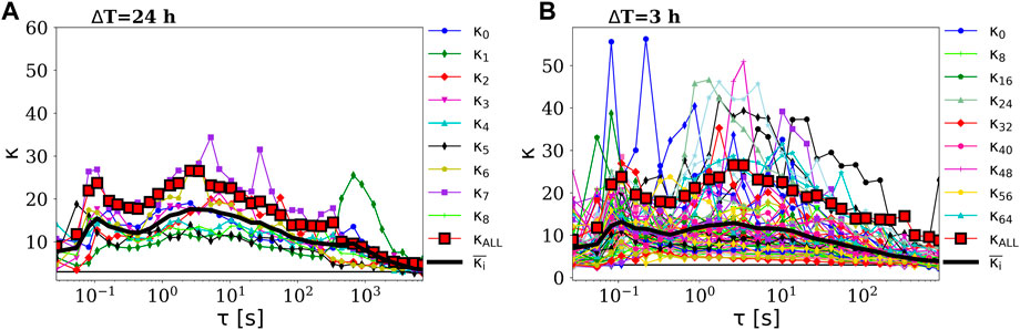
FIGURE 3. Scale dependence of κ computed for five-point increments for (A) set 1, 24 h sub-intervals and (B) set 4, 24 h sub-intervals. For many of the intervals, we observe a continuous growth of κ from scales of the order of hours to scales of [1–10] s. Then, κ decreases more abruptly toward kinetic and sub-kinetic scales, back to values of 3 (Gaussian process, black thin line). The thick black line indicates the average κ over the analyzed sub-intervals of the original data.

Because the PSP magnetic field measurements at scales below 1 s are affected by the spacecraft reaction wheels (Bowen et al., 2020; Duan et al., 2020; Dudok de Wit et al., 2020), the behavior of κ may be affected, so we limit our discussions to scales above 1 s resolution.

The questions that arise from the first step of our analysis are as follows: which κ curve illustrated in Figure 3 most accurately describes the intermittent turbulence, which is inherently a nonlinear dynamical phenomenon, observed in the slow solar wind close to the Sun? Is a data sample of several days better suited for intermittency analysis than sub-intervals spanning 24 or 3 hours? How can one decide which time interval is relevant for the analysis: one that shows low or high intermittency?

In trying to answer these questions, it became obvious that some measure of confidence should be attached to each of the estimated curves. As such, in order to better understand the high variability observed in the intermittency level of the magnetic field measured close to the Sun in a relatively short time interval (9 days) and narrow range of distances from the Sun (∼0.17–0.22 AU), we adopted a statistical method based on surrogate data, as proposed by Theiler et al. (1992). The method was designed to identify nonlinearity in time series and provides the means to evaluate the significance of the discriminating statistic (flatness), as shown below. Statistical analysis with surrogate data has been widely used in various scientific fields, from geosciences, astrophysics, and astronomy to mathematics, chemistry, medicine, and other disciplines.

The basic principle of the method involves the formulation of a null hypothesis, a possible explanation that does not appropriately describe the a priori insight data. A set of surrogate data is generated so that they are different realizations of the process consistent with the null hypothesis that we are trying to invalidate. A discriminating statistic, i.e., a number such as κ, that describes the intermittent nature of the turbulent signal can then be computed for the original and the surrogates. If the discriminating statistic of the raw data is significantly different from that of the surrogates, then we can argue with a high level of confidence that the supposed interpretation of the data assumed by the null hypothesis, is not appropriate i.e., the null hypothesis is falsified.

For non-Gaussian data, Theiler et al. (1992) suggested a generalized null hypothesis in which the underlying linear dynamics are assumed to be due to a linear Gaussian process, while the nonlinearity is due to the observation function. In this scenario, the surrogates are nonlinear, but the nonlinearity comes from the amplitude distribution and not from the dynamics. The advantage of this method is that it can point out the nature of the nonlinearity, i.e., whether it stems from the dynamics of the process or whether it comes from other sources, such as the amplitude distribution of the signal. Furthermore, in Section 3.3, we described in more detail the procedure to generate surrogate data that satisfy this null hypothesis.

3.3 Generating surrogate data for the assumed null hypothesis

In analyzing the solar wind data provided by PSP and described by the flatness illustrated in Figure 3, we generated a set of surrogate data that have the same mean, variance, and Fourier power spectrum as the original signal but whose Fourier phases are randomized, thus destroying any nonlinear correlations of the original data that resulted in the underlying dynamics of the system. The procedure involved the following steps:

1. A Gaussian time series is generated with the length, mean, and variance of the signal.

2. The original data and the Gaussian generated in Step 1 are rank-ordered by re-ordering the time sequence of the Gaussian to follow the original time series.

3. Possible nonlinear dynamics are then destroyed by phase randomization of the Fourier transform of the Gaussian rank-ordered time series.

4. Last, the original signal is reordered to match the rank order of the phase-randomized time series obtained in the previous step. This new time series represents a surrogate of the original time series.

The surrogate data generated by the steps previously described match the amplitude distribution of the original data and are therefore non-Gaussian. We estimated κ for the original data and sets of 20, 30, or 50 surrogate signals generated for Sig2. The findings are very similar for the three analyzed surrogate sets; thus, below we discuss results obtained for a set of 20 surrogates [Johnson and Wing (2005)]. We then compared κ computed for the original data with κ evaluated for the surrogates and decided whether the null hypothesis was invalidated, i.e., if κ of the original data was significantly different from that of the surrogates and took values above a confidence interval (CI) determined from the spread of κ computed for the surrogate dataset:

$\kappa >CI.(6)$

If relation (6) is satisfied, we can argue that κ describes the intermittency of the young solar wind induced by the nonlinearity in the dynamics of the fluctuations.

The confidence interval (CI) is defined as follows:

$CI=\overline{{\kappa }_{SURR}}\pm 3{\sigma }_{SURR},(7)$

where $\overline{{\kappa }_{SURR}}$ is the mean value of κ estimated for the 20 surrogates and ${\sigma }_{SURR}$ is the standard deviation of κ computed for the surrogate set.

3.4 Significance of the intermittency level quantified through κ

The scale dependence of the intermittency parameter, κ, is given in Figure 4 for the two analyzed signals: Sig1- 01–09 November 2018 and Sig2- 8 November 2018, 00:00-12:00, a chosen sub-sample of Sig1 that presents the highest level of intermittency (Figure 2, upper right panel, sub-interval number 14). The main results of our analysis are summarized in Figure 4 and described as follows:

FIGURE 4

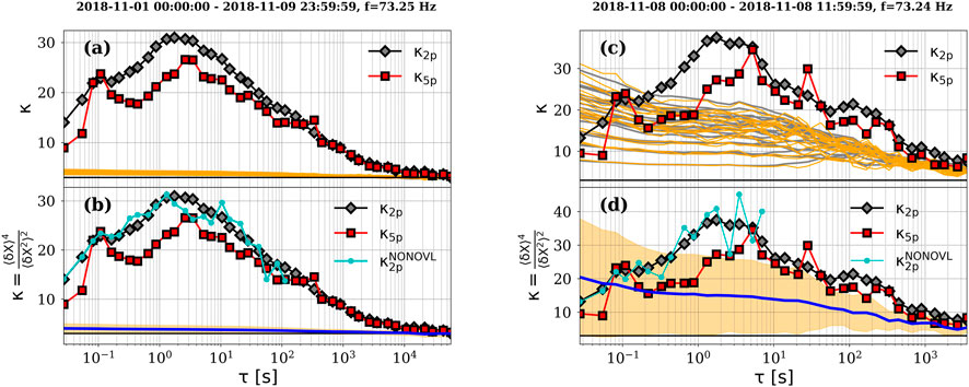
FIGURE 4. Flatness, κ, versus time scale of the magnetic energy fluctuations measured in the slow solar wind by the Parker Solar Probe. Black/red markers and lines depict κ evaluated in two-/five-point increments. Left panels, (A) and (B), show κ computed for Sig1 (01–09 November 2018 UT). Right panels, (C) and (D), show κ computed for Sig2 (8 November 2018, 00:00–12:00 UT). The horizontal black line indicates κ = 3 (Gaussian process). In the upper row of plots, (A) and (C), the gray and orange lines indicate the surrogate κ for two- and five-point increments, respectively. In the lower row of plots, (B and D), the blue line shows $\overline{{\kappa }_{SURR},}$ and the orange area indicates the confidence interval of $\overline{{\kappa }_{SURR}}\pm 3{\sigma }_{SURR}$, where $\overline{{\kappa }_{SURR}}$ and σ_SURR are the mean and the standard deviation of the five-point surrogate flatness. Cyan markers and lines in the lower panels indicate κ evaluated from non-overlapping increments of the original data.

1. The left/right panels of Figure 4 show κ computed for Sig1/Sig2 and for the ensemble of surrogates for the two approaches, two- and five-point increments. The horizontal black lines indicate the value κ = 3, the hallmark of a Gaussian process. It should be noted that κ profiles for all surrogate data constructed for Sig1 remain approximately constant and close to three at all scales, spanning roughly six decades, starting from days down to tens of milliseconds. On the other hand, the flatness of the surrogate data constructed for Sig2 spans a much broader range of values and shows a steep increase toward the smallest scales. It should be noted that Sig2 data (Figure 1, lower panel) exhibit a rather large singular structure, also referred to as a “switchback” (Dudok de Wit et al., 2020), in an otherwise stationary time series. This particular time series is an example of a short signal that includes one “extreme” event that has an important effect on both the values of κ computed for the original data and also on the spread of the κ for the surrogate set. A steeper increase of κ is observed for Sig2, which would generally be interpreted as the mark of higher intermittency, and the spread of the surrogate κ is much larger, resulting in a wide CI (Eq. 7), marked by the orange-shaded area in the lower row of plots in Figure 4.

We observed a clear difference between the behavior of the flatness computed for the original data and the one computed for surrogates. The flatness obtained for Sig1 (left column of Figure 4) was well above CI defined by the spread of the surrogates-κ, while κ computed for Sig2 was mostly undistinguishable from CI. As such, we can argue that the null hypothesis (i.e., the measure, κ, results from the linearity of the dynamics but the nonlinearity of the observation function) was invalidated for Sig1 but not for Sig2. In other words, a linear Gaussian process was revealed by the κ computed for the surrogates generated for Sig1, meaning that the randomization of the data performed to construct the surrogate destroyed the nonlinear correlations resulting from the inherent dynamics of the intermittent signal Sig1. On the other hand, the null hypothesis was not invalidated for Sig2, allowing us to argue that the observed values of κ and intermittency resided in the amplitude distribution. Therefore, we can say that the level of intermittency quantified through κ and observed in Sig2 does not fully characterize the nonlinear turbulent interactions observed in the magnetic field of the young, slow solar wind.

In order to better understand this result, we analyzed in detail the effects of the singular structure (the strong variation between 09 and 10 UT, Figure 1) on the intermittency level of Sig2 and its surrogates. We applied a data conditioning technique, as suggested by Kiyani et al. (2006), to remove extreme data outliers. The outliers were identified through a boxplot diagram as those data values that are higher than a threshold, e.g., for a standard Gaussian, 0.7% of the data are outliers. The distribution of our data was not Gaussian, and the standard boxplot diagram (not shown) identified 3.4% of the data as outliers. A data value higher than the set threshold was replaced by a flag value (i.e., 10¹⁵), which was then discarded in the statistics of the increments.

We checked the behavior of κ when we removed a) a small part of what was considered “outliers” (∼0.01% of the data), as shown in Figure 5 left, and b) all identified outliers (3.4% of the data), as shown in Figure 5 right. It should be noted how the removal of an increasing number of outliers resulted in the data becoming stationary; in addition, the spread of κ computed for the surrogates reduced, and the values became closer to 3, i.e., the surrogates became different realizations of the linear Gaussian noise assumed by the null hypothesis. Furthermore, we observed that κ computed for Sig2 decreased for all scales, even when a very small percent of the data was removed, and took values above CI when the singular structure was removed. Although the conditioned original was still intermittent, the level of intermittency, as described by the values of κ, was reduced by half compared to the unconditioned signal.

FIGURE 5

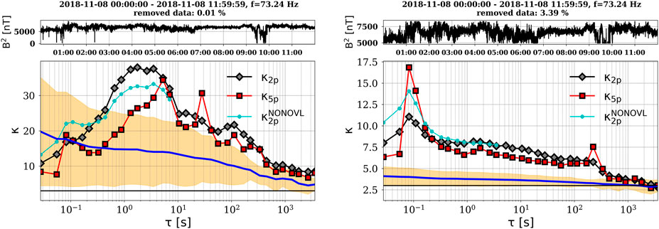
FIGURE 5. Effects of data conditioning applied on Sig2. Data are conditioned by removing extreme outliers, 0.01% (left panels) or 3.4% (right panels), Upper panels: time series of the conditioned Sig2. Lower panels: data conditioning affects both the scale dependence of κ, κ vs. τ (s), and the spread of the surrogates-κ. The horizontal black line indicates a value of κ = 3. The blue line shows $\overline{{\kappa }_{SURR}}$, and the orange area indicates the confidence interval of $\overline{{\kappa }_{SURR}}\pm 3{\sigma }_{SURR}$, where $\overline{{\kappa }_{SURR}}$ and σ_SURR are the mean and the standard deviation of the surrogates-κ. Cyan markers and lines indicate κ evaluated from non-overlapping increments.

2. Second, we performed a comparison between κ estimated from non-overlapping increments and the classical flatness determination based on overlapping increments. The cyan markers and lines in Figure 4 show the scale dependence of κ estimated from two-point non-overlapping increments. We estimated κ up to a maximum scale for which at least 4000 increments were used in the computation of the structure functions. The effects of lower statistics for the evaluation of κ at higher scales are visible in the behavior of the cyan line, where κ shows fluctuations from scale to scale. Nevertheless, we observed that κ computed from non-overlapping increments closely follows κ estimated from overlapping windows, especially at the smallest scales where the statistics for the computation of κ are identical or very similar.

The direct comparison between the two approaches, lower panels of Figure 4, black versus cyan line, respectively, confirms that κ estimated from overlapping increments is a good approximation for the evaluation of intermittency, and temporal correlations introduced by overlapping (Hnat et al., 2005) seem not to have a sizable effect on the estimation of κ.

4 A discussion on the intermittency and turbulence observed by the PSP at a close distance from the Sun

The increase in κ with decreasing scales indicates the presence of intermittency, as discussed in several previous works based on PSP data (Bale et al., 2019; Chhiber et al., 2020; Chhiber et al., 2021; Dudok de Wit et al., 2020; Horbury et al., 2020). Intermittency is confirmed by the flatness behavior illustrated in all panels of Figure 4, where κ steadily increases toward smaller scales over more than three scale decades, from hours down to seconds. All approaches, two- and five-data point overlapping differencing and non-overlapping increments, indicate the same scale dependence. In general, κ estimated from five-point increments is smaller and less smooth than when computed from two-point increments. This fact is not unexpected, as the computation of five-point increments can be seen as a moving window average resulting in a smoothing of sparse large-amplitude fluctuations, hence a smoother (less intermittent) time series of increments.

We also noted the peculiar behavior of the flatness curves, estimated both from two- or five-data points and from non-overlapping increments: at time scales of the order of several seconds (all panels of Figure 4), κ reaches a maximum value and then starts decreasing. The peak value of κ (further denoted κ_MAX) evaluated from five-point increments is generally positioned at larger time scales compared to results from a two-point increment approach. Moreover, the maximum of κ evaluated from two-point increments is generally broader and resembles a plateau distributed over several time scales. An ample analysis regarding κ_MAX and a brief review of possible sources of such a behavior of the flatness curves were performed by Roberts et al. (2022). They analyzed 20-time intervals of the solar wind magnetic field measured by the Cluster mission close to Earth, over 12 years. In another analysis of more than 3000, 5 h time intervals of magnetic field data from the PSP and Solar Orbiter, Sioulas et al. (2022) found that the maximum of κ shifts toward smaller time scales with increasing distance from the Sun, albeit with a large scatter in the distribution of the scale associated with κ_MAX.

In Figure 4, the scale dependence of κ indicates that the intermittency of the slow solar wind at a distance of 0.17 AU from the Sun starts decreasing at time scales of about 4 s. Of particular note is the distribution of κ evaluated from five-point increments (red line in Figure 4), which provides more reliable results at such small scales (Wang et al., 2020; Teodorescu et al., 2021). The scale dependence of κ estimated from two-point increments displays the same general trend as previously discussed, with the difference that a plateau is first reached at scales of several seconds down to about one second, after which a decrease in κ is observed toward the smallest scales. A peak is present in the scale dependence of κ centered around 0.1 s, but we shall not focus on sub-proton scales in this analysis. Instead, we performed further checks on the decreasing trend of κ observed over one decade of time scales between approximately [0.4, 4] s for most data samples, including the full signal, Sig1 (Figures 2–4).

Consequently, we verified the global linearity of several higher-order moments of the structure functions (SFs) over different regimes of scales. We identified SF power law regimes (linearity in log–log representation) by applying the automatic multi-order power-law-fitting algorithm—AMPA (Tam and Chang, 2011; Teodorescu et al., 2021). The power of AMPA resides in the fact that a simultaneous fit is applied to the log–log representation of SFs of several moment orders, thus ensuring the global linearity of SFs over common ranges of scales for all moment orders. The length of Sig1, more than 55 million data points, allows for a reliable estimation of SFs up to an order of q = 6 (Dudok de Wit, 2004). In Figure 6, we illustrate the SF versus scale (diamond markers) computed for Sig1 up to q = 6 together with the fitting (straight lines) and identification of several power law regimes provided by AMPA; i.e., the breaking scales between different power laws are marked by big triangles.

FIGURE 6

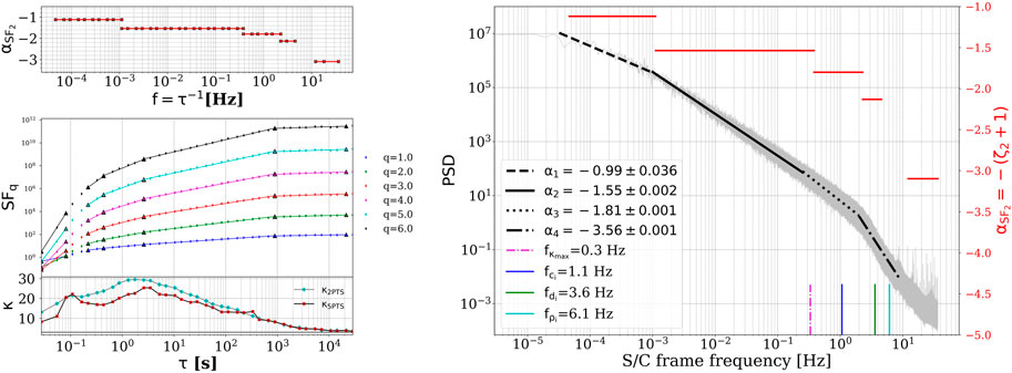
FIGURE 6. Upper left: The scaling exponents of the second-order structure function, SF₂, determined by AMPA for sub-ranges of τ [s] and transformed into frequencies as f = 1/τ [Hz]. Middle left: Scale-dependent SFs for order moments, q, up to 6 (diamond markers), and the global simultaneous fits (straight lines) over sub-ranges of scales with the same scaling exponent (power law exponent), as determined by AMPA. Lower left: Flatness, κ, as a function of τ [s]. Right: Power spectral density of the magnetic field from standard Fourier analysis applied to PSP data during its first perihelion, 01–09 November 2018. The injection, inertial, and kinetic regimes characterized by different spectral slopes are clearly separated by spectral breaks at ∼10⁻³ and 2 Hz. A steepening of the spectral slope is observed for the last decade of frequencies of the inertial range [0.25, 2] Hz, which correspond to the range of time scales where κ decreases [0.4, 4] s or [10-100] d_i. Plasma characteristic frequencies are also indicated: f_ci, f_di, and f_ρi.

The second-order SF exponents, ζ₂, computed by AMPA are transformed into spectral indices, α_SF, through the relation α_SF =-ζ₂-1 (Kolmogorov, 1941; Kolmogorov, 1962), as a function of frequency, f = 1/τ. The results shown in Figure 6 reveal that the scale dependence of the SFs up to order q = 6 displays linearity (same power law regime) over the range of scales between [0.4 and 4] s; this is precisely the range of scales for which a decrease in flatness is observed (Figure 4; Figure 6). Expressed in units of ion inertial lengths, d_i, such time scales correspond to spatial scales of the order of ∼10–100 d_i (i.e., inertial range scales), where d_i is ∼15 km and the mean flow velocity is ∼330 km/s for Sig1. The spectral indices derived from the second-order SF exponents (α_SF, Figure 6, top left) also indicate a change in power law behavior for the same frequency interval, the one corresponding to time scales in the range [0.4, 4] s, i.e., the high-frequency decade of the inertial regime, [0.25, 2.5] Hz, before the breakpoint frequency toward the kinetic regime. A steeper spectral slope α is determined by the global multi-order fit for this frequency range, α_SF = −1.8, compared to the lower frequency interval of the inertial range, [10⁻³,10⁻¹] Hz, or [100-10000] d_i, where α_SF = −1.55.

This behavior is captured by the second-order statistic, whose signature is distinguishable in the slope of the power spectral density. The traces of SF and PSD are computed and compared, i.e., the SF and PSD of the vector field components are computed, and their respective sums are then fitted. A simple transformation in the time scales into spacecraft frequencies, i.e., f = 1/τ, enables a direct comparison between the behavior of κ, or higher-order SF, over different time scales/frequency regimes and the PSD of the turbulent signal. The PSD of Sig1 is shown in Figure 6 (right). The three-scale regimes generally assumed in the classical picture of developed turbulence are very clearly delimited: the inertial regime is separated from the injection and kinetic regimes by spectral breaks observed at ∼10⁻³ Hz (also discussed by Chen et al., 2020) and 2 Hz (also discussed by Duan et al., 2020; Vech et al., 2020), respectively. It should be noted that the 4 s time scale, where the peak value of the flatness κ_MAX is observed, corresponds to a frequency of ∼0.25 Hz. A fit of the PSD in the frequency interval [0.25, 2] Hz also reveals a change in the slope of the PSD in the inertial regime: the slope becomes steeper for this last decade of frequencies in the inertial range with α_PSD = −1.81 ± 0.001. An index α_PSD = −1.55 is determined in the frequency interval [10⁻³, 2•10⁻¹] Hz. In other words, an increase in the energy transfer rate between scales is observed. Also of note is the remarkable similarity between α_PSD and α_SF.

Flatter inertial range spectra or underestimated scaling exponents have been shown to emerge when the data possess a large-scale structure (Huang et al., 2010; Carbone et al., 2018). Close to the Sun, a -3/2 inertial range turbulent spectrum has been previously reported (Chen et al., 2020; Matteini et al., 2019; Dudok de Wit et al., 2020). Analyzing whether switchbacks can be considered as part of the turbulent wave field, Dudok de Wit et al. (2020) suggested that the state of the solar wind close to the Sun is a mixture of active and quiescent conditions, both characterized by similar f^−3/2 spectra, although a shorter inertial range is observed for the pristine state.

Bowen et al. (2020), Dudok de Wit et al. (2020), and Duan et al. (2020) discussed possible effects that the PSP’s reaction wheels could have on kinetic scale measurements (or at spacecraft frequencies of the order of Hz or higher). One would expect that their effect would be a flattening of the spectral power and not the steepening we observe at scales that, nonetheless, are larger than the kinetic scales. It is, thus, reasonable to conclude that the change in behavior observed in the distribution of κ, the scale dependence of SF up to q = 6, and in the power spectrum are all manifestations of the physical phenomena taking part in the turbulent dynamics of the solar wind surveyed by the PSP.

We recall here a discussion by Borovsky and Podesta (2015) on the influence of current sheet thickness on the breakpoint frequency at kinetic scales (Chen et al., 2014) and on the spectral power at scales below the kinetic range breakpoint. It was argued that a steepening of the Fourier spectrum is observed in the vicinity of the break, accompanied by the formation of another breakpoint at a lower frequency, directly related to the thickness of the current sheets. In this context, the relation between the steepening of the power spectrum at the high-frequency end of the inertial regime, at 0.25–2 Hz, and the observed decrease of κ at corresponding time scales, [0.4–4] s or 10-100 d_i, seems to suggest that the current sheets (or switchbacks), plentifully observed in Sig1 (Dudok de Wit et al., 2020), speed up the energy transfer between scales, which in turn leads to a decrease of the intermittency level starting at inertial range scales. In addition, Chorin and Hald (2005) calculated an f⁻² inertial range turbulence spectrum when the data is populated with discontinuities.

We also checked the level of intermittency for the signal and various surrogates by fitting the scaling exponent ζ(q) via the classical log-normal cascade model (Schmitt, 2003; Medina et al., 2015; Carbone et al., 2019).

$\zeta \left(q\right)=q\mathcal{H}-\frac{\mu }{2}\left(q^2-q\right),(8)$

where μ is the intermittency parameter and ℋ =ζ(1) is the Hurst exponent. The intermittency parameter μ is ∼0.02 for classical fluid turbulence. In Figure 7, we show ζ(q) (markers) and the log-normal model fit (dashed lines) for the two scale ranges: 1) large inertial range scales (black diamonds and dashed line, respectively) and 2) small inertial range scales (red triangles and dashed line, respectively). The linear dependence ζ(q)∼qℋ, cyan, and blue lines, describing non-intermittent, monofractal behavior (Carbone et al., 2018), is shown for reference. The results for the original/surrogate data are shown on the left/right plots of Figure 7. For Sig1 and Sig2, higher intermittency is detected at larger inertial range scales, with μ ∼ 0.05, than at smaller inertial scales, where μ is slightly above 0.03. For the surrogates, a value of μ∼ 0.001 seems to indicate the absence of intermittency at all scales, except for a range of small scales of Sig2 surrogate data, where μ is closer to 0.01. This result confirms the flatness analysis that the surrogates of Sig2 still exhibit some level of intermittency, especially at smaller scales, even after the nonlinear correlations have been destroyed by the randomization procedure. The Hurst exponent takes values of 0.3 or 0.4, revealing anti-persistent fluctuations.

FIGURE 7

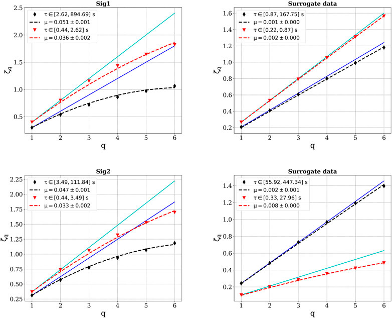
FIGURE 7. ζ(q) (markers) and the log-normal fit (dotted lines) for the original data, Sig1 and Sig2, (left) and their surrogates (right) for two sets of analyzed scales/frequencies in the inertial range.

5 Conclusion

We analyzed 9 days of high-quality magnetic field data at about 0.17 AU from the Sun. The magnetic field fluctuations were found to be highly intermittent in several previous studies (Bale et al., 2019; Bandyopadhyay et al., 2020; Chhiber et al., 2020; 2021; Dudok de Wit et al., 2020; Horbury et al., 2020), and our results are in perfect agreement with these findings. Indeed, our analysis of the flatness parameter, κ, shows a steady increase from values close to κ = 3 at scales of the order of hours (10⁵ d_i or 1 500 000 km) up to κ∼ 25 at scales of the order of seconds, i.e. 100 d_i or 1 500 km.

We evaluated the significance of this intermittency level through a statistical analysis based on the surrogate method proposed by Theiler et al. (1992). We tested whether a null hypothesis was falsified by the scale dependence of the flatness. The null hypothesis in our case was that the observed intermittency and flatness dependence on scales resulted from a linear Gaussian-like physical process, where the nonlinearity is due to the observation function. The linear process and the generation of a set of surrogate data are different realizations of this hypothesized Gaussian-like process. In this study, the discriminating statistic was represented by the flatness κ. We found that κ for the original PSP data spanning 9 days was significantly different than that of the surrogates; i.e., the null hypothesis was falsified. Thus, it can be argued that the measure (flatness) is a good descriptor of the intermittency resulting from the inherent nonlinear dynamics of the process captured by the magnetic field observations of the PSP.

The need to make such an evaluation was inspired by the variability of the intermittency level observed for a relatively narrow time period, i.e., 9 days of magnetic field observations near the Sun when sub-samples of the data were analyzed separately. Figures 2 and 3 illustrate this variability for contiguous data samples of varying lengths, from 3 to 24 hours. Some sub-intervals show very low levels of intermittency, with flat κ curves and κ values close to three, interspersed with some highly intermittent sub-intervals. For comparison, we superimposed the κ evaluated for the entire 9-day interval and saw that it did not represent the mean value of κ computed for various sub-samples. To understand this variability of intermittency, we applied the statistical apparatus of surrogates to Sig2, a 12 h data sub-sample of Sig1 that exhibited the highest level of intermittency. The high spread of the flatness for surrogates derived for Sig2 resulted in a wide confidence interval that engulfed the κ curve of the original data. The null hypothesis was not falsified in this case. As a result, the intermittency we determined for Sig2 does not fully reside in the dynamics but mostly in the amplitude distribution. Indeed, Sig2 is a non-stationary time series containing one isolated discontinuity/switchback (Dudok de Wit et al., 2020).

As further validation of this conclusion, we applied a data conditioning technique (Kiyani et al., 2006) and saw that by removing more and more of the isolated structure, the intermittency level for Sig2, in addition to the spread in surrogate flatness, decreased to the extent that the null hypothesis was invalidated; i.e., only intermittency resulted from the dynamics of the fluctuations was detected after the removal of the singular large-amplitude structure. The analysis revealed that a signal containing a relatively large number of extreme events, which are the principal manifestation of the nonlinear straining process of the turbulent cascade, resulted in a more reliable estimate of the intermittency level, while when the signal included a small number of extreme events (as is the case with Sig2, where only one such event is present) this led to an (artificial) overestimation of the intermittency. Evidently, data selection should be carefully considered. As proven in Figures 2 and 3, the automatic division of the data into samples of arbitrarily chosen lengths can lead to an under-/overestimation of the analyzed measure.

We also performed a direct comparison of the level of intermittency estimated from non-overlapping versus overlapping increments. The time scales accessible for a non-overlapping analysis with structure functions, and flatness, of Sig1, range from tens of milliseconds up to a hundred seconds and cover a relatively large part of the inertial regime. We noted that, when the statistics of increments are significant, the overlapping and non-overlapping flatness curves are very similar. This agreement between the two approaches is an indication that the correlations introduced by overlapping, as described by Hnat et al. (2005), have a negligible effect on the flatness parameter.

The intermittent nature of the young solar wind sampled by the PSP was revealed by the steady increase in κ toward small scales (of the order of seconds), from values of three at scales of several hours (10000 di) down to 4 s (100 d_i). At scales smaller than 4 s, we observed a decrease of the flatness parameter towards kinetic scales, indicative of saturation of the intermittency level. Previous works (Chian and Miranda, 2009; Wan et al., 2012a or Wu et al., 2013; Yordanova et al., 2015; Chiber et al., 2021; Roberts et al., 2022; Sioulas et al., 2022) also reported on this behavior but generally discussed the kinetic regime. We performed further checks on the behavior of κ in the time-scale interval [0.4, 4] s or [10,100] d_i. A simultaneous fit, AMPA (Tam and Chang, 2011; Teodorescu et al., 2021), of structure functions up to moment orders q = 6 seems to indicate that, indeed, in this range of time scales, the higher moments display global linearity. Moreover, second-order SF exponents, expressed as spectral indices through the relation α_SF = -ζ₂-1 (Kolmogorov, 1962; 1941), provide values remarkably similar to the power law indices obtained from a Fourier analysis of the PSD. Both methods revealed a steepening of the PSD slope in the frequency range, [0.2, 2] Hz, which covers the last decade of frequencies of the inertial regime.

The steepening of the Fourier spectrum and the formation of another breakpoint at lower frequencies are related to the presence of current sheets (switchbacks); the breakpoint frequency between the inertial and kinetic regimes is related to the thickness of these current sheets (Borovsky and Podesta, 2015). The current sheets are “active” and seem to accelerate the energy cascade at the high-frequency end of the inertial regime but reduce the intermittency in the corresponding scale range.

Data availability statement

Publicly available datasets were analyzed in this study. These data can be found at: https://cdaweb.gsfc.nasa.gov.

Author contributions

ET, ME, and JJ contributed to the conception and design of the analysis and to the interpretation of the data for the work. ET wrote the first draft of the manuscript. ME and JJ critically revised the manuscript. All authors contributed to the article and approved the submitted version.

Funding

This research was supported by the Romanian Ministry of Research, Innovation, and Digitisation, grant no. 30N/2023 (LAPAS VII) within the National Nucleus Program, the Young Researcher Program (projects 174/2020 and 87/2022), and the European Space Agency through the PRODEX program, project MISION/2021 PEA 4000134960. ME acknowledges the support of the Belgian BRAIN-BE project B2/223/P1/PLATINUM. JJ was supported by NASA grants 80NSSC22K0515, 80NSSC20K0704, 80NNSC20K1279, and 80NSSC21K1678 and NSF grant AGS2131013.

Acknowledgments

Graphical representations of the analyzed time series and a significant part of the analysis (PSD and SF computation) can be performed using the ODYN software library (Teodorescu and Echim, 2020; ODYN, RRID:SCR_023367). Online data visualization and part of the selection were conducted with the web-based data analysis service, AMDA (Génot et al., 2010).

Conflict of interest

The authors declare that the research was conducted in the absence of any commercial or financial relationships that could be construed as a potential conflict of interest.

The handling editor EY declared a past co-authorship with the author MME.

Publisher’s note

All claims expressed in this article are solely those of the authors and do not necessarily represent those of their affiliated organizations, or those of the publisher, the editors, and the reviewers. Any product that may be evaluated in this article, or claim that may be made by its manufacturer, is not guaranteed or endorsed by the publisher.

References

Alexandrova, O., Carbone, V., Veltri, P., and Sorriso-Valvo, L. (2008). Small-scale energy cascade of the solar wind turbulence. Astrophys. J. 674, 1153–1157. doi:10.1086/524056

CrossRef Full Text | Google Scholar

Anselmet, F., Gagne, Y., Hopfinger, E. J., and Antonia, R. A. (1984). High order velocity structure functions in turbulent shear flows. J. Fluid Mech. 140, 63–89. doi:10.1017/S0022112084000513

CrossRef Full Text | Google Scholar

Bale, S. D., Badman, S. T., Bonnell, J. W., Bowen, T. A., Burgess, D., Case, A. W., et al. (2019). Highly structured slow solar wind emerging from an equatorial coronal hole. Nature 576 (7786), 237–242. doi:10.1038/s41586-019-1818-7

PubMed Abstract | CrossRef Full Text | Google Scholar

Bale, S. D., Goetz, K., Harvey, P. R., Turin, P., Bonnell, J. W., Dudok de Wit, T., et al. (2016). The FIELDS instrument suite for solar probe plus. Space Sci. Rev. 204, 49–82. doi:10.1007/s11214-016-0244-5

PubMed Abstract | CrossRef Full Text | Google Scholar

Balogh, A., Beek, T. J., Forsyth, R. J., Hedgecock, P. C., Marquedant, R. J., Smith, E. J., et al. (1992). The magnetic field investigation on the ULYSSES mission: Instrumentation and preliminary scientific results. Astron. Astrophys. Suppl. Ser. 92, 221–236.

Google Scholar

Bandyopadhyay, R., Matthaeus, W. H., Parashar, T. N., Chhiber, R., Ruffolo, D., Goldstein, M. L., et al. (2020). Observations of energetic-particle population enhancements along intermittent structures near the Sun from the parker solar probe. ApJS 246, 61. doi:10.3847/1538-4365/ab6220

CrossRef Full Text | Google Scholar

Bavassano, B., and Bruno, R. (1992). On the role of interplanetary sources in the evolution of low-frequency Alfvenic turbulence in the solar wind. J. Geophys. Res. 97, 137. doi:10.1029/92JA01510

CrossRef Full Text | Google Scholar

Biskamp, D. (1993). Nonlinear magnetohydrodynamics. Cambridge: Cambridge University Press. doi:10.1017/CBO9780511599965

CrossRef Full Text | Google Scholar

Borovsky, J. E., and Podesta, J. J. (2015). Exploring the effect of current sheet thickness on the high-frequency Fourier spectrum breakpoint of the solar wind. J. Geophys. Res. Space Phys. 120, 9256–9268. doi:10.1002/2015JA021622

CrossRef Full Text | Google Scholar

Bowen, T. A., Mallet, A., Huang, J., Klein, K. G., Malaspina, D. M., Stevens, M., et al. (2020). Ion-scale electromagnetic waves in the inner heliosphere. Astrophysical J. Suppl. Ser. 246, 66. doi:10.3847/1538-4365/ab6c65

CrossRef Full Text | Google Scholar

Bruno, R., and Bavassano, B. (1991). Origin of low cross-helicity regions in the inner solar wind. J. Geophys. Res. 96, 7841–7851. doi:10.1029/91JA00144

CrossRef Full Text | Google Scholar

Bruno, R., Carbone, V., PrimaveraMalaraSorriso-Valvo, L. F. L., Bavassano, B., and Veltri, P. (2004). On the probability distribution function of small-scale interplanetary magnetic field fluctuations. Ann. Geophys. 22, 3751–3769. doi:10.5194/angeo-22-3751-2004

CrossRef Full Text | Google Scholar

Bruno, R., Carbone, V., Sorriso-Valvo, L., and Bavassano, B. (2003). Radial evolution of solar wind intermittency in the inner heliosphere. J. Geophys. Res. 108 (A3), 1130. doi:10.1029/2002JA009615

CrossRef Full Text | Google Scholar

Bruno, R. (2019). Intermittency in solar wind turbulence from fluid to kinetic scales. Earth Space Sci. 6, 656–672. doi:10.1029/2018EA000535

CrossRef Full Text | Google Scholar

Burlaga, L. (1991). Intermittent turbulence in the solar wind. J. Geophys. Res. 96, 5847–5851. doi:10.1029/91ja00087

CrossRef Full Text | Google Scholar

Carbone, F., Sorriso-Valvo, L., Alberti, T., Lepreti, F., Chen, C. H. K., Němeček, Z., et al. (2018). Arbitrary-order hilbert spectral analysis and intermittency in solar wind density fluctuations. Astrophysical J. 859, 27. doi:10.3847/1538-4357/aabcc2

CrossRef Full Text | Google Scholar

Carbone, F., Telloni, D., Bruno, R., Hedgecock, I. M., De Simone, F., Sprovieri, F., et al. (2019). Scaling properties of atmospheric wind speed in mesoscale range. Atmosphere 10 (10), 611. doi:10.3390/atmos10100611

CrossRef Full Text | Google Scholar

Case, A. C., Kasper, J. C., Stevens, M. L., Korreck, K. E., Paulson, K., Daigneau, P., et al. (2020). The solar probe Cup on the parker solar probe. ApJS 246, 43. doi:10.3847/1538-4365/ab5a7b

CrossRef Full Text | Google Scholar

Chang, T. T. S. (2015). An introduction to space plasma complexity. Cambridge University Press. doi:10.1017/CBO9780511980251

CrossRef Full Text | Google Scholar

Chen, C. H. K., Bale, S. D., Bonnell, J. W., Borovikov, D., Bowen, T. A., Burgess, D., et al. (2020). The evolution and role of solar wind turbulence in the inner heliosphere. ApJS 246, 53. doi:10.3847/1538-4365/ab60a3

CrossRef Full Text | Google Scholar

Chen, C. H. K., Leung, L., Boldyrev, S., Maruca, B. A., and Bale, S. D. (2014). Ion-scale spectral break of solar wind turbulence at high and low beta. Geophys. Res. Lett. 41, 8081–8088. doi:10.1002/2014GL062009

PubMed Abstract | CrossRef Full Text | Google Scholar

Chhiber, R., Goldstein, M. L., Maruca, B. A., Chasapis, A., Matthaeus, W. H., Ruffolo, D., et al. (2020). Clustering of intermittent magnetic and flow structures near parker solar probe’s first perihelion—a partial-variance-of-increments analysis. Astrophysical J. Suppl. Ser. 246, 31. doi:10.3847/1538-4365/ab53d2

CrossRef Full Text | Google Scholar

Chhiber, R., Matthaeus, W. H., Bowen, T. A., and Bale, S. D. (2021). Subproton-scale intermittency in near-sun solar wind turbulence observed by the parker solar probe. Astrophysical J. Lett. 911, L7. doi:10.3847/2041-8213/abf04e

CrossRef Full Text | Google Scholar

Chian, A. C.-L., and Miranda, R. A. (2009). Cluster and ACE observations of phase synchronization in intermittent magnetic field turbulence: A comparative study of shocked and unshocked solar wind. Ann. Geophys. 27, 1789–1801. doi:10.5194/angeo-27-1789-2009

CrossRef Full Text | Google Scholar

Chorin, A. J., and Hald, Ole H. (2005). Viscosity-dependent inertial spectra of the burgers and korteweg–deVries–burgers equations. PNAS 102 (11), 3921–3923. doi:10.1073/pnas.0500335102

PubMed Abstract | CrossRef Full Text | Google Scholar

Duan, D., Bowen, T. A., Chen, C. H. K., Mallet, A., He, J., Bale, S. D., et al. (2020). The radial dependence of proton-scale magnetic spectral break in slow solar wind during PSP encounter 2. ApJS 246, 55. doi:10.3847/1538-4365/ab672d

CrossRef Full Text | Google Scholar

Dudok de Wit, T. (2004). Can high order moments be meaningfully estimated from experimental turbulence measurements? PhRvE 70, 055302. doi:10.1103/PhysRevE.70.055302

CrossRef Full Text | Google Scholar

Dudok de Wit, T., Krasnoselskikh, V. V., Bale, S. D., Bonnell, J. W., Bowen, T. A., Chen, C. H. K., et al. (2020). Switchbacks in the near-sun magnetic field: Long memory and impact on the turbulence cascade. ApJS 246, 39. doi:10.3847/1538-4365/ab5853

CrossRef Full Text | Google Scholar

Echim, M., Chang, T., Kovacs, P., Wawrzaszek, A., Yordanova, E., Narita, Y., et al. (2021). “Turbulence and complexity of magnetospheric plasmas,” in Magnetospheres in the solar system. Editors R. Maggiolo, N. André, H. Hasegawa, D. T. Welling, Y. Zhang, and L. J. Paxton doi:10.1002/9781119815624.ch5

CrossRef Full Text | Google Scholar

Fox, N. J., Velli, M. C., Bale, S. D., Decker, R., Driesman, A., Howard, R. A., et al. (2016). The solar probe plus mission: Humanity’s first visit to our star. Space Sci. Rev. 204, 7–48. doi:10.1007/s11214-015-0211-6

CrossRef Full Text | Google Scholar

Frisch, U. (1995). Turbulence: The legacy of A.N. Kolmogorov. Cambridge, New York: Cambridge Univ. Press.

Google Scholar

Génot, V., Jacquey, C., Bouchemit, M., Gangloff, M., Fedorov, A., Lavraud, B., et al. (2010). Space Weather applications with CDPP/AMDA. Adv. Space Res. 45 (9), 1145–1155. doi:10.1016/j.asr.2009.11.010

CrossRef Full Text | Google Scholar

Hnat, B., Chapman, S. C., and Rowlands, G. (2005). Scaling and a Fokker-Planck model for fluctuations in geomagnetic indices and comparison with solar wind ε as seen by Wind and ACE. J. Geophys. Res. 110, A08206. doi:10.1029/2004JA010824

CrossRef Full Text | Google Scholar

Horbury, T. S., Woolley, T., Laker, R., Matteini, L., Eastwood, J., Bale, S. D., et al. (2020). Sharp alfvénic impulses in the near-sun solar wind. ApJS 246, 45. doi:10.3847/1538-4365/ab5b15

CrossRef Full Text | Google Scholar

Huang, Y., Lu, Z., Schmitt, F., Fougairolles, P., Gagne, Y., and Liu, Y. L. (2010). Second-order structure function in fully developed turbulence. PhRvE 82, 026319. doi:10.1103/PhysRevE.82.026319

PubMed Abstract | CrossRef Full Text | Google Scholar

Johnson, J. R., and Wing, S. (2005). A solar cycle dependence of nonlinearity in magnetospheric activity. J. Geophys. Res. 110, A04211. doi:10.1029/2004JA010638

CrossRef Full Text | Google Scholar

Karimabadi, H., Roytershteyn, V., Wan, M., Matthaeus, W. H., Daughton, W., Wu, P., et al. (2013). Coherent structures, intermittent turbulence, and dissipation in high-temperature plasmas. Phys. Plasmas 20, 012303. doi:10.1063/1.4773205

CrossRef Full Text | Google Scholar

Kasper, J. C., Abiad, R., Austin, G., Balat-Pichelin, M., Bale, S. D., Belcher, J. W., et al. (2016). Solar wind electrons alphas and protons (SWEAP) investigation: Design of the solar wind and coronal plasma instrument suite for solar probe plus. SSRv 204, 131–186. doi:10.1007/s11214-015-0206-3

CrossRef Full Text | Google Scholar

Kiyani, K. H., Chapman, S. C., and Hnat, B. (2006). Extracting the scaling exponents of a self-affine, non-Gaussian process from a finite-length time series. Phys. Rev. E 74 (5), 051122. doi:10.1103/PhysRevE.74.051122

PubMed Abstract | CrossRef Full Text | Google Scholar

Koga, D., Chian, A. C.-L., Miranda, R. A., and Rempel, E. L. (2007). Intermittent nature of solar wind turbulence near the Earth’s bow shock: Phase coherence and non-Gaussianity. Phys. Rev. E 75, 046401. doi:10.1103/PhysRevE.75.046401

PubMed Abstract | CrossRef Full Text | Google Scholar

Kolmogorov, A. N. (1962). A refinement of previous hypotheses concerning the local structure of turbulence in a viscous incompressible fluid at high Reynolds number. Cambridge: Cambridge Univ. Press, 82. Vol 13.

CrossRef Full Text | Google Scholar

Kolmogorov, A. N. (1941). The local structure of turbulence in incompressible viscous fluid for very large Reynolds' numbers. DoSSR 30, 301.

Google Scholar

Landau, L. D., and Lifshitz, E. M. (1971). Physique théorique, vol 6: Mécanique des fluides. Moscow: Mir.

Google Scholar

Medina, O. D., Schmitt, F. G., and Calif, R. (2015). Multiscale analysis of wind velocity, power output and rotation of a windmill. Energy Procedia 76, 193–199. doi:10.1016/j.egypro.2015.07.897

CrossRef Full Text | Google Scholar

Meneveau, C., and Sreenivasan, K., R. (1991). The multifractal nature of turbulent energy dissipation. J. Fluid Mech. 224, 429–484. doi:10.1017/S0022112091001830

CrossRef Full Text | Google Scholar

Müller, D., StCyr, O. C., Zouganelis, I., Gilbert, H. R., Marsden, R., Nieves-Chinchilla, T., et al. (2020). The solar orbiter mission: Science overview. A&A 642, A1. doi:10.1051/0004-6361/202038467

CrossRef Full Text | Google Scholar

Obukhov, A. M. (1962). Some specific features of atmospheric turbulence. J. Geophys. Res. 67, 3011–3014. doi:10.1029/JZ067i008p03011

CrossRef Full Text | Google Scholar

Parashar, T. N., Goldstein, M. L., Maruca, B. A., Matthaeus, W. H., Ruffolo, D., Bandyopadhyay, R., et al. (2020). Measures of scale-dependent alfvénicity in the first PSP solar encounter. ApJS 246, 58. doi:10.3847/1538-4365/ab64e6

CrossRef Full Text | Google Scholar

Qudsi, R., Matthaeus, W. H., Parashar, T. N., Bandyopadhyay, R., and Chhiber, R. (2020). Observations of heating along intermittent structures in the inner heliosphere from PSP data. Astrophysical J. Suppl. Ser. 246, 46. doi:10.3847/1538-4365/ab5c19

CrossRef Full Text | Google Scholar

Richardson, L. F. (1920). The supply of energy from and to atmospheric eddies. R. Soc. 97, 686. doi:10.1098/rspa.1920.0039

CrossRef Full Text | Google Scholar

Roberts, O., Varsani, A. C., Volwerk, M., Canu, P., Lion, S., and Yearby, K. (2022). Scale-dependent kurtosis of magnetic field fluctuations in the solar wind: A multi-scale study with cluster 2003–2015. JGR Space Phys. 127 (9). doi:10.1029/2021JA029483

CrossRef Full Text | Google Scholar

Schmitt, F. G. (2003). A causal multifractal stochastic equation and its statistical properties. Eur. Phys. J. B 34, 85–98. doi:10.1140/epjb/e2003-00199-x

CrossRef Full Text | Google Scholar

Sioulas, N., Huang, Z., Velli, M., Chhiber, R., Cuesta, M. E., Shi, C., et al. (2022). Magnetic field intermittency in the solar wind: Parker solar probe and SolO observations ranging from the alfvén region up to 1 AU. Astrophysical J. 934 (17), 143. doi:10.3847/1538-4357/ac7aa2

CrossRef Full Text | Google Scholar

Sorriso-Valvo, L., Carbone, V., Veltri, P., Consolini, G., and Bruno, R. (1999). Intermittency in the solar wind turbulence through probability distribution functions of fluctuations. GRL 26 (13), 1801–1804. doi:10.1029/1999GL900270

CrossRef Full Text | Google Scholar

Tam, S. W. Y., and Chang, T, T. (2011). Double rank-ordering technique of ROMA (Rank-Ordered Multifractal Analysis) for multifractal fluctuations featuring multiple regimes of scales. Process. Geophys 18, 405–414. doi:10.5194/npg-18-405-2011

CrossRef Full Text | Google Scholar

Taylor, G. I. (1938). The spectrum of turbulence. RSPSA 164, 476–490. doi:10.1098/rspa.1938.0032

CrossRef Full Text | Google Scholar

Teodorescu, E., and Echim, M. (2020). Open-source software analysis tool to investigate space plasma turbulence and nonlinear DYNamics (ODYN). Earth Space Sci. 7 (4). doi:10.1029/2019EA001004

PubMed Abstract | CrossRef Full Text | Google Scholar

Teodorescu, E., Echim, M., and Voitcu, G. (2021). A perspective on the scaling of magnetosheath turbulence and effects of bow shock properties. Astrophysical J. 910, 66. doi:10.3847/1538-4357/abe12d

CrossRef Full Text | Google Scholar

Theiler, J., Eubank, S., Longtin, A., Galdrikian, B., and Doyne Farmer, J. (1992). Testing for nonlinearity in time series: The method of surrogate data. Phys. D. 58, 77–94. doi:10.1016/0167-2789(92)90102-S

CrossRef Full Text | Google Scholar

Tu, C.-Y., and Marsch, E. (1993). A model of solar wind fluctuations with two components: Alfve´n waves and convective structures. J. Geophys. Res. 98, 1257–1276. doi:10.1029/92JA01947

CrossRef Full Text | Google Scholar

Tu, C.-Y., and Marsch, E. (1990). Evidence for a “background” spectrum of solar wind turbulence in the inner heliosphere. J. Geophys. Res. 95, 4337–4341. doi:10.1029/JA095iA04p04337

CrossRef Full Text | Google Scholar

Vech, D., Kasper, J. C., Klein, K. G., Huang, J., Stevens, M. L., Chen, C. H. K., et al. (2020). Kinetic-scale spectral features of cross helicity and residual energy in the inner heliosphere. Astrophysical J. Suppl. Ser. 246, 52. doi:10.3847/1538-4365/ab60a2

CrossRef Full Text | Google Scholar

Veltri, P., and Mangeney, A. (1999). Scaling laws and intermittent structures in solar wind MHD turbulence. Sol. Wind Nine 1999, 543–546.

CrossRef Full Text | Google Scholar

Veltri, P. (1999). MHD turbulence in the solar wind: Self-similarity, intermittency and coherent structures. Plasma Phys. control. Fusion 41, A787–A795. doi:10.1088/0741-3335/41/3a/071

CrossRef Full Text | Google Scholar

Wan, M., Matthaeus, W. H., Karimabadi, H., Roytershteyn, V., Shay, M., Wu, P., et al. (2012b). Intermittent dissipation at kinetic scales in collisionless plasma turbulence. PhRvL 109, 195001. doi:10.1103/PhysRevLett.109.195001

PubMed Abstract | CrossRef Full Text | Google Scholar

Wan, M., Osman, K. T., Matthaeus, W. H., and Oughton, S. (2012a). Investigation of intermittency in magnetohydrodynamics and solar wind turbulence: Scale-dependent kurtosis. Astrophysical J. 744, 171. doi:10.1088/0004-637X/744/2/171

CrossRef Full Text | Google Scholar

Wang, T., He, J., Alexandrova, O., Dunlop, M., and Perrone, D. (2020). Observational quantification of three-dimensional anisotropies and scalings of space plasma turbulence at kinetic scales. ApJ 898, 91. doi:10.3847/1538-4357/ab99ca

CrossRef Full Text | Google Scholar

Wawrzaszek, A., and Echim, M. (2021). On the variation of intermittency of fast and slow solar wind with radial distance, heliospheric latitude, and solar cycle. Front. Astronomy Space Sci. 7, 617113. doi:10.3389/fspas.2020.617113

CrossRef Full Text | Google Scholar

Wu, P., Perri2, S., Osman, K., Wan, M., Matthaeus, W. H., Shay, M. A., et al. (2013). Intermittent heating in solar wind and kinetic simulations. Astrophysical J. Lett. 763, L30. doi:10.1088/2041-8205/763/2/L30

CrossRef Full Text | Google Scholar

Yordanova, E., Balogh, A., Noullez, A., and von Steiger, R. (2009). Turbulence and intermittency in the heliospheric magnetic field in fast and slow solar wind. J. Geophys. Res. 114, A08101. doi:10.1029/2009JA014067

CrossRef Full Text | Google Scholar

Yordanova, E., Perri, S., Sorriso-Valvo, L., and Carbone, V. (2015). Multipoint observation of anisotropy and intermittency in solar-wind turbulence. EPL 110 (1), 19001. doi:10.1209/0295-5075/110/19001

CrossRef Full Text | Google Scholar