Global insight into a complex-structured heliosphere based on the local multi-point analysis

1 Introduction

The heliosphere is a giant bubble of magnetized plasma around the Sun. It goes beyond the Solar System and is shaped by a constant outflow of charged particles called the solar wind. Coronal mass ejections (CMEs; Webb and Howard, 2012), a gigantic eruption from the Sun, may result in large-scale heliospheric structures such as interplanetary shock (Tsurutani et al., 2003), sheath (Kilpua et al., 2017; Salman et al., 2021), magnetic flux ropes (FRs), and complex ejecta. The FRs having smooth rotating high-intensity magnetic field lines with low temperature compared to the surrounding are called magnetic clouds (MCs; Burlaga, 1988). The interplanetary CMEs (ICMEs) may interact with other ICMEs and solar wind transients, including high-speed streams (HSSs) emanating from coronal holes (CHs; Cranmer, 2009) and slow–fast stream interaction regions (SIRs; Richardson, 2018) created, while fast stream overtakes a slower stream and restructures the heliosphere in a way that may result in significant space weather disturbances (Zhang et al., 2007; Scolini et al., 2020). A study by Pal et al. (2022a) observed a structured heliosphere containing an MC and a heliospheric current sheet (HCS; Smith, 2001) that draped about the FR and resulted in ∼18% erosion of the FR flux at ∼0.5 au heliocentric distance. A study by Feng et al. (2019) indicated that a large-scale FR could occur in the heliosphere by merging multiple ICME FRs. CME interaction with solar wind structures can impact their properties in several ways such as rotating their axis (Manchester IV et al., 2004; Nieves-Chinchilla et al., 2012; 2013; Isavnin et al., 2013; Heinemann et al., 2019; Pal et al., 2020), deforming their front convexity (Braga et al., 2022), and distorting and eroding their intrinsic magnetic properties (Pal et al., 2021; Pal, 2022). If a CME originates close to CHs, its expansion and propagation are prohibited in the direction of CH open fields and its propagation path is deflected by the magnetic gradient resulting from the difference in the magnetic field strength of the surrounding flux system (Manchester et al., 2017; Heinemann et al., 2019). These effects alter the initial ICME properties close to the Sun and can lead to significant errors in predictions of ICME arrival time and geoeffectiveness (Pal et al., 2022b).

A comprehensive understanding of the Sun–Earth system leads to improvements in the prediction of phenomena that have significant societal relevance. This calls for improvement in tools such as data assimilation, statistical analysis, and synthesis of observations and models (Daglis et al., 2021). Several studies have analyzed interacting large-scale solar wind phenomena using multi-point observations supported by heliospheric modeling and their space weather impacts (Farrugia et al., 2011; Winslow et al., 2021; Pal et al., 2022b). However, the existence of a series of solar wind transients (similar or different kinds) and their interactions are not very usual. Farrugia et al. (2011) studied an ICME followed by the corotating interaction region (CIR—SIRs that persist for several solar rotations) using three longitudinally separated spacecraft and found distortion and rotation of ICME FR caused by its interaction with the CIR. Shugay et al. (2018) compared the predicted and observed arrival time and speed of HSSs continued for three consecutive Carrington rotations (CRs), where, during one of the CRs, the HSS overtook a complex ejecta formed of merged ICMEs that resulted in significant decrement in the HSS speed. However, the models used in their prediction were unable to capture the impact of the HSS–ejecta interaction. Scolini et al. (2021) investigated the CME–HSS interaction using a heliospheric model in two radially aligned spacecraft and derived CME complexity driven by the HSS. Winslow et al. (2021) studied the CME–SIR interaction using observations from two spacecraft having longitudinal conjunction and determined drastic changes in the ICME magnetic structure and properties of sheath due to the interaction. Palmerio et al. (2022) studied two successive ICMEs followed by HSS on their way to Earth and Mars and found out the reason for the second ICME missing Mars being the ICME’s rotation and deflection due to its interaction with the HSS. Moreover, all these studies focused on understanding the complexity resulting from interacting transients and serve as an indicator for further investigations on the interacting solar events in the heliosphere.

The present study uncovers the features of a complex-structured heliosphere formed of a series of solar wind transients and their interactions using a longitudinally separated multi-point remote and in situ observations aided by heliospheric modeling. The structured heliosphere caused a disturbance in space weather, influencing the loss of multiple satellites on 3 February 2022 (Dang et al., 2022; Fang et al., 2022; Hapgood et al., 2022; Tsurutani et al., 2022). By probing the origin, early and inner-heliospheric evolution of the components of the structured heliosphere, we infer its complexity and explain its unalike appearances in distant in situ observations. Moreover, this study provides evidence of solar transient evolution regulating its global structure and local impacts. In Section 2, we provide a brief overview of the satellite instruments, the dataset utilized in this study, and a summary of the observed structured heliosphere. In Section 3, we analyze the data and their outcome. Finally, in Section 4, we discuss our results and present our conclusions.

2 Instruments, dataset, and event overview

This study employs multi-viewpoint extreme ultraviolet (EUV) and white-light solar imagery, heliospheric images, and multi-point in situ observations aided by the Wang-Sheeley-Arge (WSA)-ENLIL+Cone model publicly available for simulation runs by the Community Coordinated Modeling Center (http://ccmc.gsfc.nasa.gov). The model consists of a semi-empirical WSA (Arge and Pizzo, 2000; Arge et al., 2004) coronal model that approximates the solar wind outflow at an inner boundary 21.5 Rs and a magnetohydrodynamical (MHD) ENLIL solar wind model (Odstrčil et al., 1996; Odstrčil and Pizzo, 1999a; Odstrčil and Pizzo, 1999b; Odstrcil, 2003; Odstrcil et al., 2004) that provides a time-dependent description of the background solar wind plasma and magnetic field. CME-related transients are then inserted at the inner boundary as high-pressure (without magnetic field) pulses. The CME geometry is approximated with a cone model described by Zhao et al. (2002) and Xie et al. (2004).

To obtain multi-point remote-sensing data, we use Extreme UltraViolet Imager (EUVI), Cor2 coronagraph and Heliospheric Imager-1 (HI-1; Eyles et al., 2009), onboard the Sun-Earth Connection Coronal and Heliospheric Investigation (SECCHI; Howard et al., 2008), suite of the Solar Terrestrial Relations Observatory Ahead (STEREO-A; Kaiser et al., 2008) spacecraft, C2&C3 coronagraphs of the Large Angle and Spectrometric COronagraph (LASCO; Brueckner et al., 1995) onboard the Solar and Heliospheric Observatory (SOHO; Domingo et al., 1995), the Atmospheric Imaging Assembly (AIA; Lemen et al., 2012) and Helioseismic and Magnetic Imager (HMI; Scherrer et al., 2012) instruments onboard the Solar Dynamics Observatory (SDO; Pesnell et al., 2012), and H-α imagery from the National Solar Observatory (NSO)/Global Oscillation Network Group (GONG) instrument.

We use in situ observations of solar wind plasma, interplanetary magnetic field (IMF), Suprathermal Electron Telescope (STE), Magnetometer (MAG), Solar Electron and Proton Telescope (SEPT) on board IMPACT (Luhmann et al., 2008) suite of STEREO-A, Magnetometer (Horbury et al., 2020), Energetic Particle Detector (EPD; Rodríguez-Pacheco et al., 2020) and Solar Wind Analyzer (SWA; Owen et al., 2020) suites onboard Solar Orbiter (SolO; Müller et al., 2020), Magnetic Field Investigation (MFI; Lepping et al., 1995), Solar Wind Experiment (SWE; Ogilvie et al., 1995), 3D Plasma Analyzer (3D-P; Lin et al., 1995) instruments onboard Wind (Lepping et al., 1995), EPAM (Electron, Proton, and Alpha Monitor), and SWICS (Solar Wind Temperatures, Speeds, Composition, and Charge States) onboard Advanced Composition Explorer (ACE; Smith et al., 1998).

The level-2, 1-min resolution in situ data are collected from the public Automated Multi-Dataset Analysis (AMDA; Génot et al., 2021), Coordinated Data Analysis Web (CDAWeb), and the ACE Science Center (ASC) databases. During the 7-day period centered on the structured heliosphere, STEREO-A and SolO were 0.6 $(\sim 34°)$ and 0.26 au $(\sim 18°)$ eastward from the Lagrangian point-L1 at 0.96 and 0.85 au heliocentric distances, respectively, with a spread in heliographic latitudes (−2.7°, −2.1°, −6° for STEREO-A, SolO, and Wind, respectively). In Figure 1A, C and Figure 2A, the in situ observations using multiple spacecraft are shown, whereas in Figure 1B and Figure 2B, the location of the spacecraft and the CME directions in Heliocentric Earth Equatorial (HEEQ) are indicated.

FIGURE 1

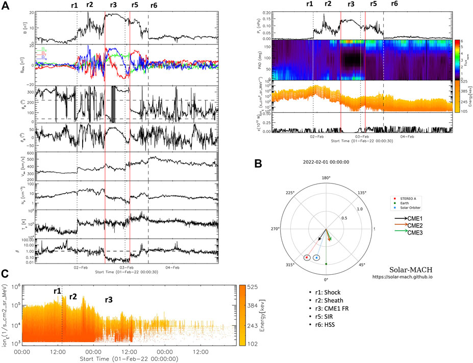
FIGURE 1. (A) Solar wind magnetized plasma measurements (in the RTN coordinate system) obtained from STEREO-A are divided into two panels. The left panel contains magnetic field intensity (B) and vector components (B_RTN), magnetic vector angles (ϕ_B and θ_B), plasma velocity (V_sw), density (N_p), temperature (T_p), and proton-β (from top to bottom). The right panel shows total pressure (P_t), PAD of the suprathermal electron at 246–255 eV energy range, energetic ion (ion_E) (100–500 eV) intensities from the Sunward telescope (please note that STEREO-A is upside down at the moment of this event), and ϵ. The ϕ_B between the horizontal lines corresponds to the sunward IMF. The vertical lines separate the annotated regions. The annotated regions are described at the right. (B) Locations where in situ measurements were obtained are shown in the ecliptic plane using colored dots where the center indicates the location of the Sun. Three arrows show the direction of CME propagation longitudes obtained from remote observation. The location of STEREO-A and the Solar Orbiter is encircled. (C) ion_E measurements from the Solar Orbiter with annotated regions. The measurements of solar wind magnetic field and plasma were not available from the solar wind.

FIGURE 2

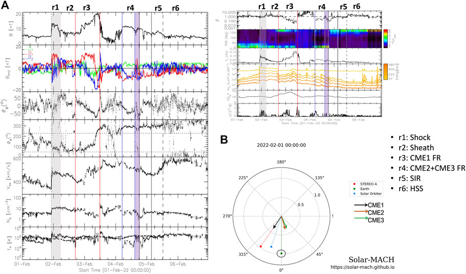
FIGURE 2. (A) Solar wind measurements divided into two panels. The observations are obtained using Wind and ACE at L1 (in the GSE coordinate system). The left panel contains the intensity and vector components of B, θ_B, ϕ_B, V_sw, N_p, and T_p. The right panel shows β, PAD, P_t, ion_E, mean iron charge state $<Q_{Fe}>$, and ϵ. The ϕ_B between horizontal lines corresponds to anti-sunward IMF. The grey-shaded region shows an abundance of a mini FR, whereas the purple-shaded region indicates the interaction region between two FRs. In (B), the location of L1 is encircled.

2.1 Overview of the structured heliosphere

2.1.1 In situ observations

We analyzed the in situ measurements of solar wind magnetic properties such as magnetic vector (B), total intensity (B), field line latitude (θ_B) and longitude (ϕ_B) angles, plasma properties, including plasma velocity (V_sw), density (N_p), temperature (T_p), suprathermal electron pitch angle distribution (PAD) at 246–255 eV energy range, and energetic ion (∼ 100–550 KeV) intensities (ion_E), and mean iron charge state (⟨Q_Fe⟩) during the passage of the structured heliosphere. At STEREO-A and L1, we derive the proton-β (the ratio of solar wind proton pressure to the magnetic pressure), total perpendicular pressure (P_t; proton thermal pressure + magnetic pressure perpendicular to the magnetic field (Russell et al., 1990)) of solar wind from in situ measurement, and the ϵ parameter that is sometimes used to describe the upstream solar wind Poynting flux transfer to the magnetosphere during the geomagnetic storm and sub-storm processes (Akasofu, 1981; Koskinen and Tanskanen, 2002). The ϵ (Akasofu, 1981) parameter is a coupling function that is used to describe the relationship between solar wind condition and magnetospheric disturbances and depends on V_sw, B, and clock angle q of the solar wind magnetic field oriented perpendicular to the Sun–Earth line, i.e., tan  θ_c = B_y/B_z (Perreault and Akasofu, 1978; Akasofu, 1979), and a scale factor l₀ = 7R_E (R_E–Earth radii) that is understood as a constant effective area of the solar wind–magnetosphere interaction $(ϵ=V_{sw}{B}^2/4\pi {\sin }^4({\theta }_c/2)l_0^2)$. However, ϵ is a first-order approximation and is not adequate to provide the description of total energy transfer (Koskinen and Tanskanen, 2002). The higher value of ϵ at L1 during the crossing of the complex-structured heliosphere complies with the fact that the structure was geoeffective. At STEREO-A, we derive the ϵ parameter to estimate the geomagnetic consequences that might occur if the structure at STEREO-A would have impacted Earth. Figure 1A, C and Figure 2A show the in situ measurements and derived parameters obtained from STEREO-A, SolO, and Wind & ACE, respectively. The STEREO-A, SolO, and Earth locations are represented by red, blue, and green color dots, respectively, on the ecliptic plane (panel B of Figures 1 and Figure 2), where the Sun locates at the center. The measurements in STEREO-A and SolO are collected in the radial, tangential, normal (RTN) coordinate, whereas at the Lagrangian point-L1, it is obtained in the geocentric solar ecliptic (GSE) coordinate. Unfortunately, due to spacecraft interference, except ion_E, the continuous level-2 data from SolO for solar wind plasma and magnetic properties were not available.

The arrival of the compound heliospheric structure was identified by a sudden enhancement (region r₁) in B, V_sw, N_p, T_p, P_t, and ion_E on 1 February 2022, at 22:20 and 22:00 UT at L1 and STEREO-A, respectively. The r₁ was followed by an interval r₂ having increased magnetic field fluctuations and enhanced ion_E. The r₁ and r₂ regions were identified at SolO using the enhanced ion_E patches. The horizontal lines in ϕ_B panels indicate the sector boundaries (SBs). The field lines crossing one of the nominal boundaries indicate a change of their directions toward the sector or vice versa (in RTN). The same is identified by the change of the propagation direction of the suprathermal electrons from the field aligned to anti-field-aligned or vice versa. At STEREO-A, inside the region r₂, during 2:00–8:00 UT on 2 Feb 2022, B and P_t significantly enhanced with B having multiple intensity dips and the ϕ_B crossed the SBs multiple times, whereas at L1, the field lines remain in between the SBs for the interval.

r₂ was followed by a region r₃ having smooth coherent rotation in B and high intensity B, N_p less than the ambient medium and proton-β < 1, indicating the presence of a FR. During r3, the presence of bidirectional suprathermal electrons and a decrease in ion_E were observed at both L1 and STEREO-A. Also, at SolO, low-energy ion_E started decreasing at ∼01:00UT on 2 February 2022, which may suggest the beginning of region r₃. During r₃, the ⟨Q_Fe⟩ peaked at L1. At L1, r3 was followed by high V_sw, N_p, and proton-β, where suprathermal electron PAD was isotropic. A region r₄ showing FR-like properties with comparatively high intensity B, large coherent magnetic field rotation, low N_p, T_p, and proton-β was observed only at L1. However, these were not observed at STEREO-A. A region indicated by r₅ was observed at both L1 and STEREO-A, where V_sw was increasing, P_t reached a local maximum, and T_p showed enhancement. After r₅, V_sw significantly increased (region r₆). From the PAD data at both L1 and STEREO-A, it was evident that IMFs directed toward the Sun during r₅ and r₆.

2.1.2 Remote-sensing observations

Taking into account the arrival time and speed of different segments in the structured heliosphere at the Sun, we identified three consecutive CMEs—CME1, CME2, and CME3—and a nearby CH as responsible origins of the transients in the structured heliosphere. Only CME1 was associated with an eruptive M-class flare that occurred at 22:30 UT on 29 January 2022, from a bipolar active region (AR) identified as NOAA 12936 and located at N17E11 in the heliographic coordinate.

Figures 3–5 show the white-light images of CME1, CME2, and CME3 using coronagraphs and their sources identified on the solar disk using running-difference EUV images. CME1 appeared as a halo event at t_cme1 ∼ 00:40 UT on 30 January 2022, with a distorted shape identified by their leading edges visible at STEREO-A/COR2 and LASCO/C2 field-of-view (FOV) (Figures 3A, B). Figures 3C, D CME1 in COR2 and LASCO/C3 coronagraphs around 3 h after its first appearence, where the leading edges of the two different parts of CME1 were not clearly observed. Using coronal EUV images, we could locate only one post-eruption arcade and a “J”-shaped ribbon at the CME1 eruption location. Therefore, we may assume that CME1 was not accompanied by any other CME and that the two leading edges observed at coronagraphs (STEREO-A/COR2 and LASCO/C2) were associated with CME1. However, CMEs may generate, having no direct association, with AR, and they may lack classic low-coronal signatures Robbrecht et al. (2009).

FIGURE 3

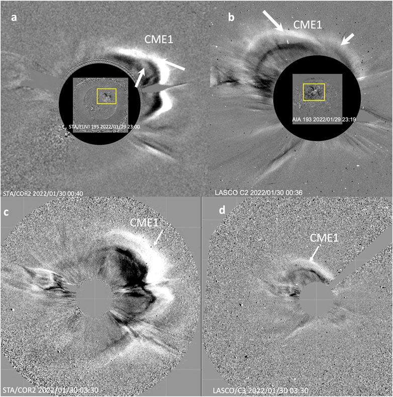
FIGURE 3. White-light observations of CME1 in STEREO-A/COR2 (A) and LASCO/C2 (B) at its first appearance when two separate structures associated with CME1 can be identified well. In the lower panel, the observation of CME1 is shown using STEREO-A/COR2 (C) and LASCO/C3 (D), 3 h after its first appearance. In the upper panel, the CME’s two distinct parts (CME1₁ and CME1₂) are indicated with white arrows. At the upper panel, the running-difference EUV image of the solar disk during CME2 eruption is shown, where the CME1-associated coronal signature is pointed using a yellow box.

FIGURE 4

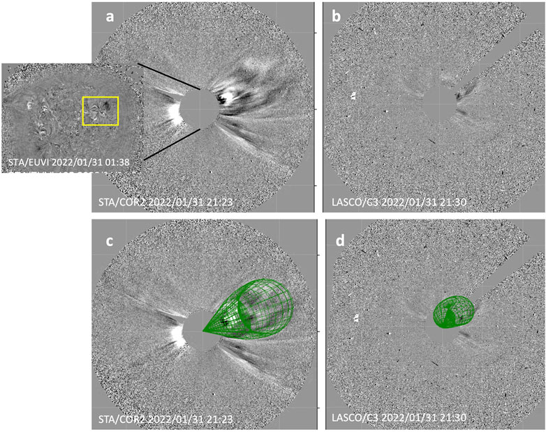
FIGURE 4. White-light observations of CME2 observed in STA/COR2 (A) and LASCO/C2 (B) and fitted with GCS approximation (C, D). In the inset of (A), the running-difference EUV image during CME2 eruption is shown. The associated coronal signature is indicated using a yellow box.

FIGURE 5

FIGURE 5. White-light observations of CME3 observation by STA/COR2 (A) and LASCO/C2 (B) and its approximation with GCS shown in (C, D). In the inset of (A), the running-difference EUV image during CME3 eruption is shown. The yellow box indicates the CME3-associated coronal brightening.

The origin of CME2 and CME3 was associated with AR 12936, while it rotated toward the west and reached locations N17W21 and N17W34, respectively (the insets of Figures 4, 5). The CMEs appeared with their full-grown structures in LASCO/C2 FOV at t_cme2 ∼ 17:50 UT on 31 January 2022 and t_cme3 ∼ 08:20 UT on 1 February 2022, respectively. The low-coronal signatures are shown using a yellow box overplotted on the EUV difference images. For CME1 and CME2, we identified coronal dimming regions on the solar disk, and for CME3, a coronal brightening was observed at the north–west solar limb. The distorted leading edge (LE) of CME1 is well observed at STEREO-A/HI-1. In Figures 6A, B, we show the STEREO-A/HI-1 (FOV diameter 20 deg) running-difference images where the LEs of CME1, CME2, and CME3 are identified distinctly at position angles 271 deg (CME1 LE) and 277 deg (CME2 and CME3 LEs) and are indicated with white arrows. Figure 6C shows a time–distance plot of the ICME LEs. The LEs are tracked at a position angle (PA) corresponding to the propagation longitude of the CME trajectories. The errors in measuring the PAs provide the uncertainty in deriving the propagation distance of ICME LEs with time (Figure 6C).

FIGURE 6

FIGURE 6. Front edges of CME1 (A) and CME2 and CME3 (B) as observed by STA/HI-1. (C) Time–distance plot of CME1, CME2, and CME3. The front edges of CME2 and CME3 began to interact at $\sim 7:00$ UT on 2 February 2022.

The flare origin AR 12936 was closely followed by another bipolar AR 12938 and a CH that was located to the southeast of AR 12938. The CME1 eruption was accompanied by a “J”-shaped flare-ribbon (Démoulin et al., 1996) and a forward EUV-sigmoid (Titov and Démoulin, 1999) observed at SDO/AIA 1600 A⁰ and 131 A⁰, respectively, which indicate that the ICME FR had right-handed (RH) twisted field lines. In Figures 7A, B, the EUV images of the solar disk obtained from STEREO-A/EUVI 195Å and SDO/AIA 193Å are shown with the CH overplotted on them using white contours. The CH faced STEREO-A (within ±20° of the central meridian) around the time of CME1 eruption, whereas it faced the SDO around the eruption of CME3. The indicated bright regions shown with arrows are associated with the two ARs. The CH boundary was obtained following the method described by Rotter et al. (2012) and Rotter et al. (2015). They found a strong relationship between the CH close to the CME and solar wind high-speed stream peak amplitudes. We notice that the CH in our study took ∼2 days to rotate $\sim 34°$ to appear near the disk center of the Earth-facing solar disk. Similarly, the HSS originating from the CH arrived at L1 ∼2 days after its arrival at $\sim 34°$ east to L1, i.e., the location of STEREO-A.

FIGURE 7

FIGURE 7. (A) STA/EUVI 195Å and (B) SDO/AIA 193Å observations of the solar disk when the coronal hole overplotted using white contours appeared within ±20° of CM. The grids are drawn with ±20° separation in the Stonyhurst coordinate system.

3 Analysis and results

3.1 In situ analysis

Section 2.1.1 describes multi-point in situ observations of different substructures (regions) in the structured heliosphere. Here, we described r₁–r₅ regions exhibiting different behaviors. In this section, we explain each region based on our analysis.

Region r₁ observed at all locations indicates the arrival of a shock driven by CME1 FR. The shock can accelerate charged particles (Giacalone, 2012) and cause ion enhancements. In our study, we considered a particular ion energy range ($\sim 100--500$ eV), at which the measurements of the ion’s number density are available for all three locations. Region r₂ corresponds to a sheath that contains a wealth of substructures that are swept into and compressed by CME1 while propagating outward from the Sun. The sheath observed by STEREO-A contains multiple HCS crossings associated with the patches of ion_E enhancements, isotropic PAD of suprathermal electrons, and high-density piled-up compression region (r₂ in Figure 1A). However, the sheath at L1 did not contain HCS crossing, whereas at its front, the abundance of a small-scale FR (mini-FR; indicated by the grey-shaded region in Figure 2A) can be speculated by the signature of almost smoothly rotating magnetic field components and a high intensity B coinciding its front part with the strongest ion_E enhancement. A mini-FR showing similar criteria was observed in a recent study by Kilpua et al. (2021). However, the mini-FR was not identified by STEREO-A. The two patches of ion_E enhancements observed by SolO (the region indicated by r₂ in Figure 1C) might correspond to the presence of the mini-FR and multiple HCS crossings, respectively. Although, due to the unavailability of solar wind magnetic field and plasma data, we could not confirm it.

Region r₃ contains the FR of CME1 that appeared with mostly negative and positive B_z at L1 and STEREO-A, respectively. Inside r₃, the signature of BDE was observed in both L1 and STEREO-A. Also, CME1 propagated as an individual structure with a separation angle between the ICME legs larger than the angular distance between the location of STEREO-A and L1. Therefore, we assume that the same FR was present in region r₃. Following Burlaga’s (1988) definition of a magnetic cloud, we confidently identified the FR’s front and rear boundaries in the solar wind data and obtained its axis orientation in both locations by fitting its vector magnetic profile with four different techniques—minimum variance analysis (MVA; Sonnerup and Scheible, 1998), a constant α linear force-free (LFF; Lepping et al., 1990; Marubashi and Lepping, 2007) cylindrical model, a circular and elliptical cylindrical model based on the radial dependence of the current density (CC and EC Nieves-Chinchilla et al., 2016, 2018), and the Three-Dimensional COronal Rope Ejection (3DCORE; Weiss et al., 2021a; Weiss et al., 2021b) model based on the assumption of a uniformly twisted torus-shaped flux rope with a global circular shape attached to the Sun. The LFF, CC, EC, and 3DCORE fitting to CME1 FR are shown in Figures 8A–D, where the left and right panels contain the fittings on observed magnetic field vectors obtained by Wind and STEREO-A, respectively. The inclination angle (θ_GSE- angle measured positive toward north from the ecliptic plane) and the azimuth angle (ϕ_GSE- angle measured counterclockwise positive from the Earth–Sun direction) of the CME1 axis, impact parameter (Y₀ − perpendicular distance between the FR axis and the spacecraft propagation path normalized to the FR radius), and handedness (H), estimated at L1 and STEREO-A by FR-fitting, are mentioned in Table 1. In MVA, Y₀ is approximated as Y₀ = ⟨B_x,FR⟩/⟨B⟩ (Démoulin and Dasso, 2009; Ruffenach et al., 2015). Here, B_x,FR is in the FR frame obtained using MVA. We confirm the certainty in the MVA method by calculating the intermediate-to-minimum eigenvalue ratio. The ratio is more than 2 (Sonnerup and Scheible, 1998), which indicates that the CME1 FR axis orientation is unambiguously determined using MVA. The error in the fitting of the LFF model is measured using $E_{\text{rms}}={\left({\sum }_{i=1}^N{\left[{\mathbf{B}}_{\text{obs}}(t_i)-{\mathbf{B}}_{\text{LFF}}(t_i)\right]}^2\right)}^{1/2}/\left(N\max |{\mathbf{B}}^{\text{obs}}|\right)$ (Marubashi and Lepping, 2007). For CC and EC, the model fit errors are estimated using ${\chi }_{CC/EC}^2={\sum }_{i=1}^N{\left[\left({\mathbf{B}}_{\text{obs}}^2(t_i)-{\mathbf{B}}_{\text{CC/EC}}^2(t_i)\right]\right)}^{1/2}/N$ (Nieves-Chinchilla et al., 2016; 2018). Here, N is the number of points inside the FR included in the analysis. The estimated error values in fitting CME1-FR at two separate locations using different models indicate a good fit (for Wind observations, the E_rms, ${\chi }_{CC}^2$, and ${\chi }_{EC}^2$ are 0.27, 0.39, and 0.4, and for STA, the values are 0.23, 0.2, and 0.19, respectively). At L1, the FR appeared as an intermediate FR (Palmerio et al., 2022) with an inclination angle of 36° ± 4°, and the low value of Y₀ indicates that the FR crossed with its core. The presence of the FR core was evident from the increased abundance of the high-charge state [⟨Q_Fe⟩ > 12 Lepri et al. (2001)]. However, at STEREO-A, it appeared as a highly inclined FR with an inclination angle of 58° ± 8° to the ecliptic plane.

FIGURE 8

FIGURE 8. Left and right panels show the observation of solar wind magnetic field vectors in GSE and RTN coordinates at L1 and STEREO-A using Wind and STEREO-A spacecraft, respectively. The green, red, and blue colors represent B_x (B_R), B_y (B_T), and B_z (B_N), respectively. The fitting with LFF (A), CC (B), EC (C), and 3DCORE (D) models is overplotted on the CME1 FR bounded by two vertical lines.

TABLE 1

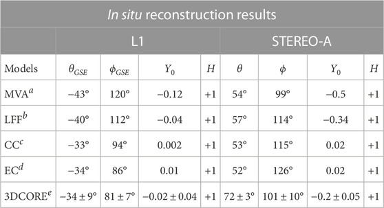
TABLE 1. Summary of results obtained from in situ reconstruction of CME1 FR observed by Wind and STEREO-A spacecraft.

A significant mismatch in the FR inclination at two different locations (Table 1) indicates a complexity in the CME1 FR that might result from the early and/or interplanetary FR evolution. An increase in ion_E close to the FR rear boundary at L1 and STEREO-A coincides with a shock-like region featured by an enhancement in B, P_t, and gradually increasing V_sw caused by the impact of the HSS behind it.

At L1, region r₄ contains the signatures of multiple interacting FRs with a large and nearly smooth rotation in B_z. It suggests that the region was formed of two merged FRs (indicated by shaded regions in Figure 2A) corresponding to CME2 and CME3 with a boundary region $(r_4^{\prime })$ between them having depression in B and enhancement in N_p and proton-β. A similar region inside a merged FR was identified by Feng et al. (2019). A negative-to-positive rotation in B_z and almost negative B_y suggest that the FR had a right-handed twist and intermediate-to-low-inclination to the ecliptic plane. The FR’s orientation was further confirmed using MVA, which gave θ_GSE = −28° and ϕ_GSE = 278° with an intermediate-to-minimum eigenvalue ratio of 4. The absence of a significant enhancement in ⟨Q_Fe⟩ during r₄ suggests that the merged FR did not cross the L1 with its core. Region r₅ contains a local peak in P_t, a decreasing N_p, gradually increasing V_sw and T_p, and local peak at B. This satisfies the SIR identification criteria suggested by Jian et al. (2006), Lepping et al. (1997), and Yermolaev et al. (2022). Yermolaev et al. (2022) performed a superposed epoch analysis of solar wind parameters for corotating interaction regions (CIRs) with and without a preceding interplanetary shock wave during high and low solar activity periods and observed a decrease in n_p and enhancement in T_p, B, V_sw, and thermal pressure. However, they found that the temporal profile of β remains at nearly 1 during the CIR crossings. At STEREO-A observation, the rear part of region r₅ contains a local dip in B, peak in β, T_p, and N_p, and the ϕ_B’s sudden crossing of one of the sector boundaries, which further suggests an existence of the HCS crossing at that region (Smith, 2001; Pal et al., 2022a). The presence of SIR at region r₅ suggests that the HSS originating from the nearby CH overtook the comparatively slow-speed stream ahead of it. Region r₆ following r₅ contains the HSS, where V_sw reached more than 500 km/s in both L1 and STEREO-A. The region showed similar characteristics to a high-speed stream that followed and compressed the rear region of an MC studied by Lepping et al. (1997). At r₆, T_p was comparatively high, N_p was low at STEREO-A and had a gradually decreasing profile at L1, and B reached to average and resulted in a comparatively higher β than that of the preceding region.

3.2 Remote-sensing analysis

In the interplanetary medium, before reaching in situ observation points, we tracked the propagation of CMEs in heliocentric distance 0.05– ∼0.4 AU using the STEREO-A/HI-1 imager. We extracted the time-elongation plots for the CMEs and converted them to the time-distance plots using the harmonic mean (HM; Lugaz et al., 2009) method. This method requires the Sun-observer distance, elongation angle, and the angle (ϕ_HM) between the sun-observer line and the LE trajectory. We determined ϕ_HM using the CME propagation direction (θ_lat, ϕ_lon) at the maximum observable height h_LE from a forward modeling method (Thernisien et al., 2006; Thernisien et al., 2009) using LASCO/C2, C3 and STEREO-A/COR2 images. We consider that after h_LE ∼ 20Rs, the CME propagation direction is constant in the heliosphere. From the propagation of CMEs as observed in the heliographic images (Figures 6A, B) and the time–distance plot (Figure 6C) derived from the heliographic images, it is evident that CME1 propagated individually without having an interaction with other CMEs. However, CME3 caught up to the CME2 speed at a heliocentric distance of ∼ 0.35 ± 0.02 au as CME3 had a higher early speed (573 km/s) than that of CME2 (465 km/s) derived by fitting the height–time plot of ICME LEs in coronagraphs.

The CMEs observed in coronagraphs are modeled using Graduated Cylindrical Shells (GCSs; Thernisien et al., 2006) having croissant-like shapes to understand the three-dimensional morphology of their FRs. The fits are performed to quasi-simultaneous images from different viewpoints covering the height range of 6–20 Rs to obtain the geometry of CMEs and their propagation directions. We derived their physical parameters including θ_lat, ϕ_lon, aspect ratio (κ), half angular width (AW), tilt (λ—measured counterclockwise positive from the solar west), and the height of the leading edge, h_LE. An analysis of the errors in the CME 3D parameters arising from the human-in-the-loop factor has recently been presented by Verbeke et al. (2022). In the analysis of the CME1, Dang et al. (2022) fitted the whole structure of CME1 using a single GCS. Instead, we used two separate GCSs to fit CME1₁ and CME1₂. The use of multiple GCS models to fit a single structure has been carried out previously to better reproduce the complex appearance of a CME in the coronagraph field-of-view (Rodríguez-García et al., 2022). In movie m1 (“m1. mov”) and m2 (“m2. mov”) attached with this paper, we show GCS approximations of CME1₁ and CME1₂ during the interval 2022/01/30 00:23–2022/01/30 03:38. In the lower panels of Figures 4, 5, we display the GCS approximation of CME2 and CME3, respectively.

Columns 1–5 of Table 2 list the GCS-fitting results for three CMEs. Here, the results in row 1 are derived by a single GCS approximation of CME1 as carried out by Dang et al. (2022). Row 2 contains the fitting results where CME1 is approximated with two different GCS structures. Rows 3 and 4 contain GCS-fit results for CME2 and CME3, respectively. To investigate the atypical shape of CME1 associating two distinct structures in coronagraphs (Section 2.1.2), we concentrated on interpreting CME1’s solar origin and its early evolution. To obtain the footpoints of the CME in the low-corona (Dissauer et al., 2019), we captured the extent of coronal dimming—regions of strongly reduced emission at EUV (Hudson et al., 1996; Sterling and Hudson, 1997)—by using cumulative dimming masks during the interval started at the time of flare onset and ended, while the CME appeared as a full-grown structure in coronagraphs. The dimming masks contain all pixels having intensity below a certain threshold obtained following the work of Reinard and Biesecker (2008).

TABLE 2

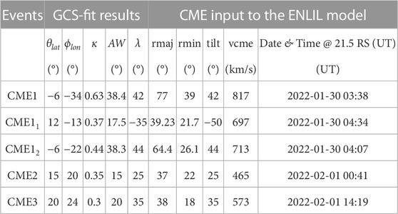
TABLE 2. CME parameters obtained from GCS approximations and converted to the WSA-ENLIL+Cone model input.

The dimming region is indicated using a red contour on the STEREO-A/EUVI image in Figure 9A. It surrounds both ARs 12936 and 12938, which further suggests that CME1 eruption resulted due to an interplay between two ARs. We notice that the southeastern part of the red contour in Figure 9A was in close proximity to a CH (shown in white in Figure 9A) that might initially deflect the FR structure. The two bipolar ARs are shown using HMI magnetogram in the lower panel of Figure 9A, where the outward and inward magnetic field line regions are indicated by white and black patches, respectively. The polarity inversion line (PIL) is overplotted with a red line. We notice that the PIL exists only on AR 12936 and the radial magnetic field component B_r of AR 12938 barely crossed the noise threshold. It further suggests that AR 12936 is stronger than AR 12938. Figure 9B shows extrapolated closed coronal field lines connected to AR 12936 and AR 12938. The coronal field lines are obtained using the potential field source surface (PFSS; Wang and Sheeley, 1992) model. We utilize the pfsspack1 https://www.lmsal.com/∼derosa/pfsspack/ IDL library to perform PFSS extrapolations. Figure 9C shows a running-ratio composite image prepared with STEREO-A/EUVI 195, 284, 171 Å images, where the dashed white line indicates the wavefront of the pseudo-wave generated from the expanding outer envelope of the propagating CME (Olmedo et al., 2012) and the coronal hole region is shown in black. The locations of L1, SolO, and STEREO-A during the structured heliosphere interval are projected on the solar disk using cyan, blue, and red dots, respectively. Based on the derived orientation of the CME1 FR axis (Table 1) at two different locations, L1 and STEREO-A, we approximated the global structure of CME1 FR and represented the same in Figure 9D. The global FR structure approximated from its in situ observations matches well with the FR’s imprints on running-ratio composite images and coronagraphs.

FIGURE 9

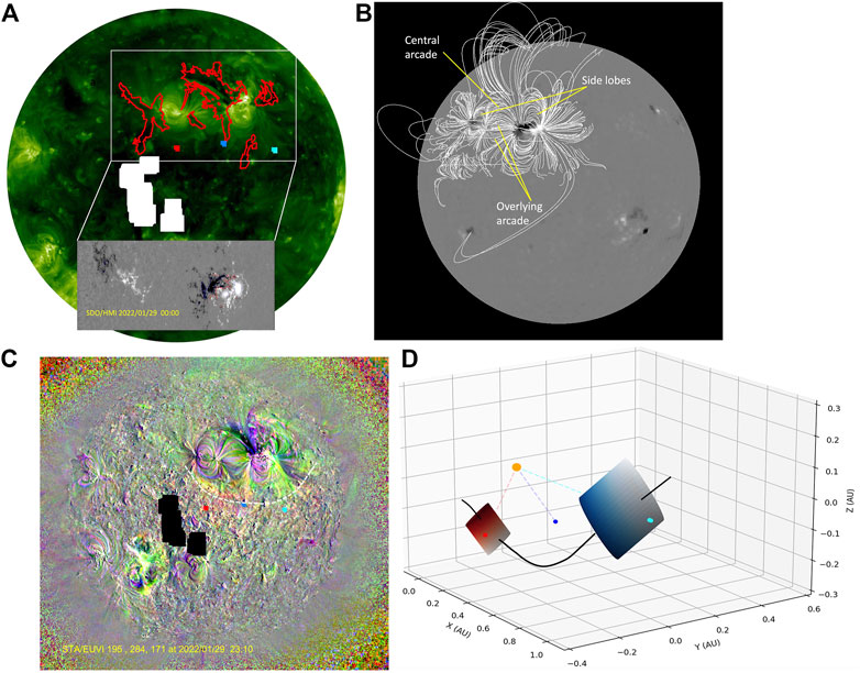
FIGURE 9. (A) Coronal dimming region (red contour) formed during CME1 eruption is overplotted on the STA/EUVI 195Å image along with the coronal hole shown in white. The white-outlined box contains both ARs which are shown in the SDO/HMI magnetogram. The polarity inversion line is shown using a red contour overplotted on the magnetogram. The blue contours enclose regions with a radial magnetic field B_r greater than the noise threshold. (B) Coronal field extrapolation till 2.5 Rs using PFSS. The white field lines are closed field lines associated with AR 12936 and 12938. The different arcades derived using PFSS are named as central arcade, side lobes, and overlying arcade following the 3D cartoon of a typical breakout configuration shown in Chen et al. (2016). (C) CME1 wavefront is indicated by the white dotted line on a running-ratio composite image, where the presence of a coronal hole is shown using a red-filled contour. (D) Sketch of the CME1 FR’s global shape where the right and left circular cross-sectioned cylinders are used to show the FR’s orientation and size at L1 and STEREO-A, respectively. The locations of L1, SolO, and STEREO-A are projected on the solar disk and shown using cyan, blue, and red color dots on all panels.

3.3 Heliospheric modeling analysis

To understand the structured heliosphere’s behavior, we simulated the solar wind conditions in 0.1–2 au radial, −60° − +60° latitudinal, and 0°–360° longitudinal extents, during 29 January 29–7 February 2022. We used the WSA-ENLIL+Cone model available at NASA’s CCMC that couples the WSA (version 5.2) model’s synoptic maps computed from the time-dependent sequence of daily updated GONG synoptic magnetograms with the ENLIL (version 2.8f) model having the default ambient solar wind condition setting (“a6b1”) and the CME kinematics and speed derived from the GCS fitting at 21.5 Rs. Columns 6–10 in Table 2 show the CME parameter translation from the GCS output to the ENLIL input following the process discussed in Nieves-Chinchilla et al. (2022). The WSA-ENLIL+Cone model is strongly influenced by the CME inputs (Mays et al., 2015; Kay et al., 2020), errors and uncertainty in ambient model parameters, and solar wind background derived using coronal maps.

We obtained two simulation results, S₁ and S₂, using two sets of CME input parameters, where for S₁, we considered CME1 as a single structure while approximated with GCS, and for S₂, we used two separate GCSs to reconstruct the two parts of CME1—CME1₁ and CME1₂. In Figures 10A, B, we provide snapshots of ENLIL simulation results in the ecliptic plane before and after the merging of CME2 and CME3, respectively. Figures 10C–E show the comparison of simulated solar wind parameters with the in situ observation at L1, SolO, and STEREO-A, respectively. The simulation results from S₁ and S₂ (the simulations are available at S1 https://ccmc.gsfc.nasa.gov/results/viewrun.php?domain=SH&runnumber=Sanchita_Pal_082022_SH_1 and S2 https://ccmc.gsfc.nasa.gov/results/viewrun.php?domain=SH&runnumber=Sanchita_Pal_092922_SH_1) are represented in purple and red colors, respectively. Table 3 summarizes the results of the comparison of the shock arrival at L1, SolO, and STEREO-A derived from S₁ and S₂ (the simulations are available at S1 https://ccmc.gsfc.nasa.gov/results/viewrun.php?domain=SH&runnumber=Sanchita_Pal_082022_SH_1 and S2 https://ccmc.gsfc.nasa.gov/results/viewrun.php?domain=SH&runnumber=Sanchita_Pal_092922_SH_1) to its observed arrival times and speeds. The negative signs in the values of columns 5 and 6 indicate that the simulated arrival time of the shock (r₁) at L1 and SolO is later than the observed, and the simulated arrival speeds are less than those of the observed ones. By comparing the S₂ simulation results to the observations, we find that the simulated shock arrival time and speed were within ± 4 h and ± 50 km/s of those of the observed values, respectively. The errors in prediction are within the mean absolute error range that Wold et al. (2018) found in their study, where they used the WSA-ENLIL+Cone model in prediction of the ICME arrival time at L1, STEREO-A, and STEREO-B during the interval of March 2010 and December 2016.

FIGURE 10

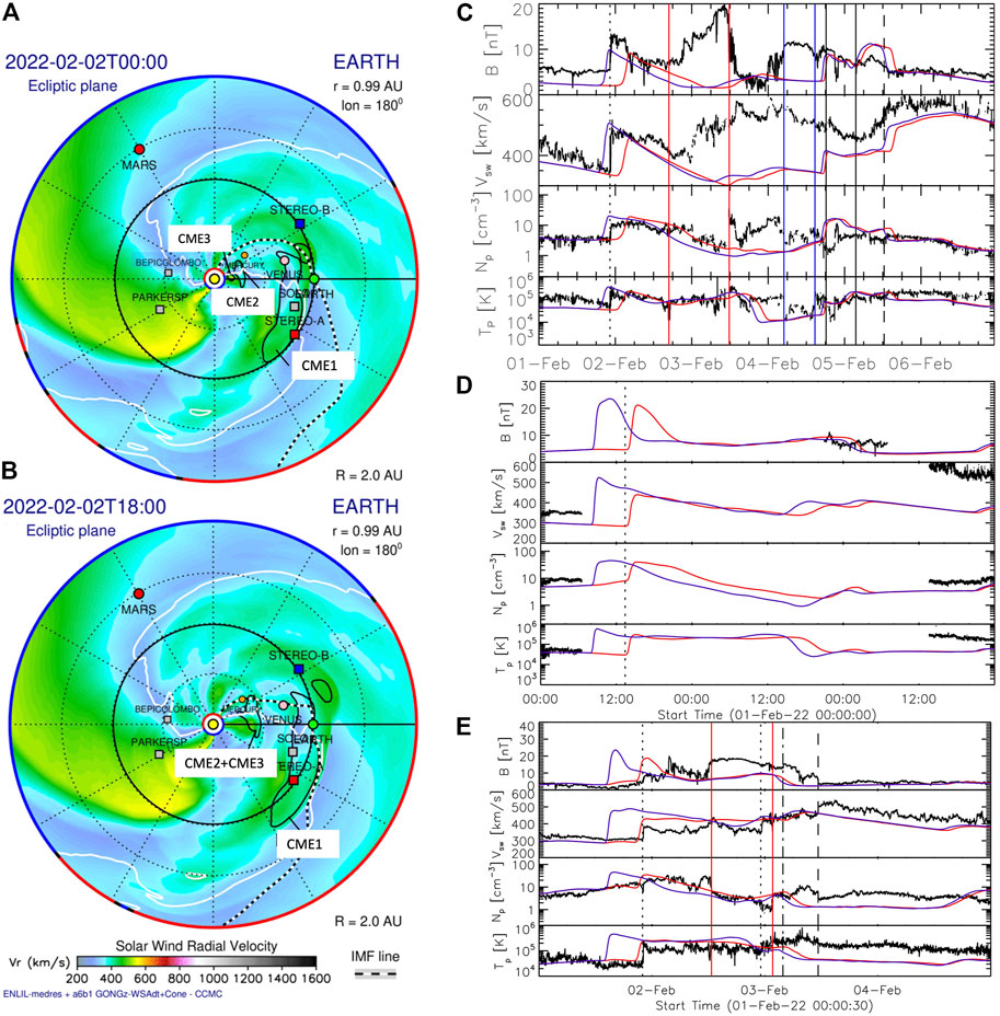
FIGURE 10. Overview of the WSA-ENLIL+Cone simulation result at three locations. (A,B) Snapshots of the simulation (S₂) results for the radial speed Vr shown in the ecliptic plane before and after merging of CME2 and CME3, respectively. The white contours represent the simulated location of HCS. (C–E) Solar wind plasma parameters such as magnetic field intensity (B), solar wind speed (V_sw), density (N_p), and temperature (T_p) derived from S₁ and S₂ simulations are overplotted on real observations using purple and red lines, respectively. The vertical lines explain the boundaries of the regions described in Section 3.

TABLE 3

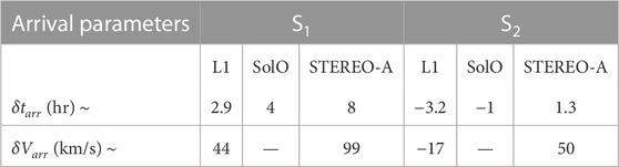
TABLE 3. Summary of results obtained from the comparison between the simulated and real arrival speed (δV_arr) and time (δt_arr) of the structured heliosphere at different locations.

The speed of HSS that we obtained using the model was ∼50 km/s lower than the observed value at both L1 and STEREO-A. However at L1, the modeled solar wind parameters specifically, B and V_sw, were significantly different from the observed ones at r₄ and the region in between r₃ and r₄. The modeled and observed solar wind speed difference at the region between r₃ and r₄ was $\sim 200$ km/s. Shugay et al. (2018) used WSA-ENLIL+Cone simulation to model an HSS speed while the HSS interacted with merged ICMEs. As the model could not capture the interaction well, they found the difference between the modeled and observed speeds of the HSS as 217 km/s.

4 Discussion and conclusion

Using multi-point remote and in situ analysis combined with global simulations, this study uncovers a complex compound heliospheric structure triggered by several large-scale structures. The part of the structure that impinged Earth caused multiple moderate geomagnetic storms. Interestingly, we found that the properties of the structure varied significantly in different longitudinally separated locations, which further indicates that the structure’s impacts on different locations might not be the same. This study leads to an enhanced understanding of the global properties of compound heliospheric structures and the reasons behind the disparities in their local properties.

At L1, the structured heliosphere contained six different components including an interplanetary shock, a sheath followed by an individual and merged FRs associated with CME1 and CME2+CME3, respectively, an SIR, and an HSS. The total energy input to the magnetosphere during the crossing of the structured heliosphere through L1 was approximated as W_ϵ = ∫ϵ(t)dt = 4.3 × 10¹⁴ W (Perreault and Akasofu, 1978). At STEREO-A, the structured heliosphere contained four regions except the CME2 + CME3 FR. If the structure appeared at STEREO-A hit Earth, W_ϵ could decrease by a factor of 25 from its derived value at L1. From the ion_E parameter, only the presence of shock, sheath, and CME1 FR was approximated at SolO.

Close to the CME1 FR rear boundary, a shock-like/compression wave structure was observed that matches to what Lepping et al. (1997) and Scolini et al. (2020) found inside FRs which was followed by an SIR and a CME, respectively. The CME–CME interaction studied by Scolini et al. (2020) reported a shock inside the preceding CME. The shock amplified the CME’s B_z significantly and resulted in an intense geomagnetic storm. In our case, the shock-like structure amplified the southward magnetic field component of CME1 FR by $\sim 8$ nT observed at both L1 and STEREO-A. This structure was driven by a following HSS and a merged FR at L1.

The WSA-ENLIL+Cone simulation allowed us to reconstruct the propagation scenario of multiple interacting solar wind transients in the inner heliosphere till 2 au. It shows the presence of an HSS behind the eastern part of CME1 and a merged CME2+CME3 behind the western part of CME1. The solar wind speed observed at r₆ and in between r₃ and r₄ at L1 was almost similar. The observation suggests that the merged CME2 + CME3 structure was overtaken by the following HSS, which further penetrated in between r₃ and r₄, pushed ICME1 from behind, and caused instability inside the ICME1 FR. However, from the simulation result, the HSS behavior of overtaking the merged CME2 + CME3 structure was not confirmed. Although the simulated results had good agreement with the observed arrival time and speed of the shock driven by ICME1, the simulation could not capture well the merged ICME (CME2 + CME3)’s arrival time and its interaction with the HSS at L1. From the observational analysis, we could confirm that unlike CME1, the merged ICME structure crossed L1 with its flank discussed in (Section 3.1), although simulation results did not fully agree with it. According to the simulation, the merged ICME crossed L1 not so far from its apex, the density of the complex-merged ICME was higher than the surroundings and became an obstacle for the HSS. Therefore, the HSS remained behind the merged ICME while arrived at L1.

The comparison between the observed and modeled solar wind features demonstrates that this type of modeling approaches can successfully reproduce the large-scale features of the structured solar wind, but have a number of limitations that must be considered while modeling their interactions. The Cone model of CME is a hydrodynamic structure, and it is inserted into the inner ENLIL boundary (21.5 R_s) as a cloud of spherical plasma with uniform plasma properties (Mays et al., 2015). The structure gradually expands with time and evolves in the presence of surrounding solar transients. At the inner boundary, the modeled CME lacks an internal (driver) magnetic field, and as a result, the ENLIL+Cone model may tend to overestimate the plasma density and temperature of the propagating structure and underestimate the magnetic field strength (Xie et al., 2012). Including the internal magnetic field is essential for accurately capturing the physics of an ICME’s evolution and its solar wind interaction in transit (Luhmann et al., 2020). Also, the model of ambient corona that is used to drive the ambient solar wind model majorly utilizes the processed line-of-sight (LOS) magnetograms of the Earth-facing solar disk. Riley et al. (2012) and MacNeice et al. (2018) discussed in more detail the limitations of the data inputs available to these models, assessed the possible error sources in the modeling, and speculated the way of mitigation of these problems in the future.

At L1, the FR axis orientation matched well with the tilt of CME1₁ (obtained using GCS), the post-eruption arcade that appeared as a coronal signature of the CME eruption at AR12936 observed using SDO/AIA 193Å during 00:00-06:00 UT on 30 January 2022, and the AR’s PIL (see Figure 9A). At STEREO-A, the FR axis direction matched well with the tilt of CME1₂ (obtained from the GCS-fitting result). However, we could not locate any post-eruption arcade and PIL on the corona whose tilt could be matched with the tilt of CME1₂. Although stealth CME can erupt without leaving any coronal signature, it is not straightforward to relate the field-line orientation inside the FR observed by STEREO-A with another CME that could possibly erupt from the multipolar flux system connected to AR 12936 and AR 12938. Thus, we speculate that CME1₂ was a part of CME1 and resulted from the deflection of the eastern part of CME1 due to interaction with the nearby CH. The coronal wave’s structure shown in Figure 9C suggests that due to the open magnetic field configuration of the CH located at the southeast of AR pairs, the CME’s eastern part underwent a deflection toward the north (Olmedo et al., 2012; Heinemann et al., 2019). At a height of 8 Rs, the eastern part of CME1 was observed to be inclined with ∼ − 36° (measured clockwise negative from the solar west), whereas the western part was inclined with $\sim 44°$ deg to the ecliptic plane.

To obtain the footprints of CME1 and its initial behavior, we derived coronal dimming regions (red contour in Figure 9A) resulting from CME1 eruption. The dimming regions surrounded two consecutive bipolar ARs (AR-12936 and AR-12938). From the extrapolated coronal field lines obtained using PFSS (Figure 9B), we confirm that AR 12936 and AR 12938 formed a multipolar flux system (central arcade and side lobes), where a null point was formed between an energized low-lying sheared arcade (central arcade) and an overlying arcade with an opposite polarity. Chen et al. (2016) proposed a 3D cartoon for a typical breakout configuration (Figure 1A). The multipolar flux system in our case resembles the arcade geometry described in that figure quite well. In such a configuration, reconnection can occur when the low-lying sheared arcade rises and compresses the current layer around the null point (Antiochos et al., 1999; Lynch et al., 2004; Reinard and Biesecker, 2008; Karpen et al., 2012). This leads to reconnection that causes flux transfer from the restraining overlying arcade to the neighboring side lobes and reduces the confining force acting on the flux system. The reduced overarching force can further trigger an explosive flare-reconnection at the side lobes with favorable conditions (Lynch and Edmondson, 2013; Pal et al., 2022a). In our case, CME1 eruption that was accompanied by an M-class flare might have followed the eruption mechanism described previously. The flare signature was prominent at AR12936, which was a strong magnetic region in the whole flux system. We also observed a filament between the two ARs (below the low-lying arcade) using GONG/H-α imagery. However, the filament might not be a source of any other eruption because it was almost static due to the increased magnetic tension resulting from the reconnection between neighboring sidelobes and was not observed to rise above and erupt. It went through “slow-dissolution” during 4:52–5:45 UT on 30 January 2022, after the CME1’s eruption took place. The disappearance of filaments may occur when the rate of its mass loss to the chromosphere increased the rate of new mass accumulation (Martin, 1973).

Using multi-point solar and heliospheric observations coupled with heliospheric modeling, this work aims to understand the anatomy of a complex-structured heliosphere that includes several large-scale interacting heliospheric structures like CMEs, SIR, and HSS. Thanks to the facility of multiple simultaneous solar and heliospheric remotes and in situ observations that allowed us to understand the components of the structured heliosphere and their interplay. The period considered for this analysis was led by a CME which had significantly unalike appearances at two distant locations—at STEREO-A and L1. At L1, the range of electromagnetic energy (ϵ) that was transferred from the solar wind during 2–5 February 2022 was 0.1–2 × 10¹² W. In general, during magnetic storms, the energy exceeds 10¹² W and may intermittently reach up to 10¹³ W (Koskinen and Tanskanen, 2002). In our case, the evolution and impact on Earth of the structured heliosphere resulted in two minor geomagnetic storms, which are believed to influence the loss of satellites owned by an aerospace manufacturing company Space-X. During the same interval, $\sim 0.6$ au eastward to the L1, the total transferred electromagnetic energy W_ϵ was significantly lesser than that at L1. Therefore, this study supports the employment of multi-point remote and in situ observations along with the heliospheric modeling in studying interacting heliospheric events to infer their global structures and improve the predictability of space weather.

Data availability statement

The datasets presented in this study can be found in online repositories. The names of the repository/repositories and accession number(s) can be found as follows: Automated Multi-Dataset Analysis (AMDA; http://amda.irap.omp.eu/index.html), Coordinated Data Analysis Web (CDAWeb; https://cdaweb.gsfc.nasa.gov/), the ACE Science Center (ASC; https://izw1.caltech.edu/ACE/ASC/level2/index.html) database, and the STEREO Science Center (SSC; https://stereo-ssc.nascom.nasa.gov/data.shtml). This work made use of ESA's JHelioviewer Müller et al. (2017) software. The GCS approximation of CMEs are performed using https://github.com/johan12345/gcs_python/tree/0.2.2 GCS Python (DOI: 10.5281/zenodo.5084818). Gieseler et al. (2023) is used to demonstrate the location of spacecrafts. The heliospheric model simulations are performed in Community Coordinated Modeling Center (CCMC; https://ccmc.gsfc.nasa.gov/).

Author contributions

SP, TNC, LB, EK, and FC contributed to the conception and design of the study. SP, LB, AW, and TNC performed the analysis. All authors contributed to preparing the manuscript and approved the submitted version.

Funding

SP acknowledges the support of NASA Solar Orbiter Collaboration and STEREO missions. TNC acknowledges the support of the NASA Solar Orbiter, STEREO, PSP missions, and Heliophysics Internal Fund (HIF) programs. CM was funded by the European Union (ERC, HELIO4CAST, 101042188).

Acknowledgments

SP thanks Dr. James A Klimchuk for the useful discussion on the solar origin of the CMEs, Dr. Erika Palmerio for her help initially with the Community Coordinated Modeling Center (CCMC) model run, and Dr. Katsuhide Marubashi for providing us with the linear force-free cylindrical model. TNC, SP, and FC acknowledge the scientific discussion within the LASSOS-Goddard group. The WSA and Enlil models were developed by C. N. Arge (currently at NASA/GSFC) and D. Odstrcil (currently at GMU), respectively. The authors would like to thank the model developers and the Community Coordinated Modeling Center (CCMC) staff. The authors also acknowledge the Solar Orbiter, SDO, NSO, SOHO, and STEREO teams.

Conflict of interest

The authors declare that the research was conducted in the absence of any commercial or financial relationships that could be construed as a potential conflict of interest.

Publisher’s note

All claims expressed in this article are solely those of the authors and do not necessarily represent those of their affiliated organizations, or those of the publisher, the editors, and the reviewers. Any product that may be evaluated in this article, or claim that may be made by its manufacturer, is not guaranteed or endorsed by the publisher.

Author disclaimer

Views and opinions expressed are, however, those of the author(s) only and do not necessarily reflect those of the European Union or the European Research Council Executive Agency. Neither the European Union nor the granting authority can be held responsible for them.

Supplementary material

The Supplementary Material for this article can be found online at: https://www.frontiersin.org/articles/10.3389/fspas.2023.1195805/full#supplementary-material

References

Akasofu, S. I. (1981). Energy coupling between the solar wind and the magnetosphere. Space Sci. Rev. 28, 121–190. doi:10.1007/BF00218810

CrossRef Full Text | Google Scholar

Akasofu, S. I. (1979). Interplanetary energy flux associated with magnetospheric substorms. Planet. Space Sci. 27, 425–431. doi:10.1016/0032-0633(79)90119-3

CrossRef Full Text | Google Scholar

Antiochos, S. K., DeVore, C. R., and Klimchuk, J. A. (1999). A model for solar coronal mass ejections. Astrophysical J. 510, 485–493. doi:10.1086/306563

CrossRef Full Text | Google Scholar

Arge, C. N., Luhmann, J. G., Odstrcil, D., Schrijver, C. J., and Li, Y. (2004). Stream structure and coronal sources of the solar wind during the May 12th, 1997 CME. J. Atmos. Solar-Terrestrial Phys. 66, 1295–1309. doi:10.1016/j.jastp.2004.03.018

CrossRef Full Text | Google Scholar

Arge, C. N., and Pizzo, V. J. (2000). Improvement in the prediction of solar wind conditions using near-real time solar magnetic field updates. J. Geophys. Res. 105, 10465–10479. doi:10.1029/1999JA000262

CrossRef Full Text | Google Scholar

Braga, C. R., Vourlidas, A., Liewer, P. C., Hess, P., Stenborg, G., and Riley, P. (2022). Coronal Mass Ejection Deformation at 0.1 au Observed by WISPR. Astrophys. J. 938, 13. doi:10.3847/1538-4357/ac90bf

CrossRef Full Text | Google Scholar

Brueckner, G. E., Howard, R. A., Koomen, M. J., Korendyke, C. M., Michels, D. J., Moses, J. D., et al. (1995). The large angle spectroscopic coronagraph (LASCO). Sol. Phys. 162, 357–402. doi:10.1007/BF00733434

CrossRef Full Text | Google Scholar

Burlaga, L. F. (1988). Magnetic clouds and force-free fields with constant alpha. J. Geophys. Res. 93, 7217–7224. doi:10.1029/JA093iA07p07217

CrossRef Full Text | Google Scholar

Chen, Y., Du, G., Zhao, D., Wu, Z., Liu, W., Wang, B., et al. (2016). Imaging a magnetic-breakout solar eruption, 820, L37. doi:10.3847/2041-8205/820/2/L37

CrossRef Full Text | Google Scholar

Cranmer, S. R. (2009). Coronal holes. Living Rev. Sol. Phys. 6, 3. doi:10.12942/lrsp-2009-3

PubMed Abstract | CrossRef Full Text | Google Scholar

Daglis, I. A., Chang, L. C., Dasso, S., Gopalswamy, N., Khabarova, O. V., Kilpua, E., et al. (2021). Predictability of variable solar-terrestrial coupling. Ann. Geophys. 39, 1013–1035. doi:10.5194/angeo-39-1013-2021

CrossRef Full Text | Google Scholar

Dang, T., Li, X., Luo, B., Li, R., Zhang, B., Pham, K., et al. (2022). Unveiling the space weather during the starlink satellites destruction event on 4 february 2022. Space weather. 20. e2022SW003152. doi:10.1029/2022SW003152

CrossRef Full Text | Google Scholar

Démoulin, P., and Dasso, S. (2009). Magnetic cloud models with bent and oblate cross-section boundaries. Astronomy Astrophysics 507, 969–980. doi:10.1051/0004-6361/200912645

CrossRef Full Text | Google Scholar

Démoulin, P., Priest, E., and Lonie, D. (1996). Three-dimensional magnetic reconnection without null points: 2. Application to twisted flux tubes. J. Geophys. Res. (Space Phys. 101, 7631–7646. doi:10.1029/95ja03558

CrossRef Full Text | Google Scholar

Dissauer, K., Veronig, A. M., Temmer, M., and Podladchikova, T. (2019). Statistics of coronal dimmings associated with coronal mass ejections. II. Relationship between coronal dimmings and their associated CMEs. Astrophys. J. 874, 123. doi:10.3847/1538-4357/ab0962

CrossRef Full Text | Google Scholar

Domingo, V., Fleck, B., and Poland, A. I. (1995). The SOHO mission: An overview. Sol. Phys. 162, 1–37. doi:10.1007/BF00733425

CrossRef Full Text | Google Scholar

Eyles, C. J., Harrison, R. A., Davis, C. J., Waltham, N. R., Shaughnessy, B. M., Mapson-Menard, H. C. A., et al. (2009). The heliospheric imagers onboard the STEREO mission. Heliospheric Imagers Onboard STEREO Mission 254, 387–445. doi:10.1007/s11207-008-9299-0

CrossRef Full Text | Google Scholar

Fang, T.-W., Kubaryk, A., Goldstein, D., Li, Z., Fuller-Rowell, T., Millward, G., et al. (2022). Space weather environment during the SpaceX starlink satellite loss in february 2022. Space weather. 20, e2022SW003193. doi:10.1029/2022SW003193

CrossRef Full Text | Google Scholar

Farrugia, C. J., Berdichevsky, D. B., Möstl, C., Galvin, A. B., Leitner, M., Popecki, M. A., et al. (2011). Multiple, distant (40°) in situ observations of a magnetic cloud and a corotating interaction region complex. J. Atmos. Solar-Terrestrial Phys. 73, 1254–1269. doi:10.1016/j.jastp.2010.09.011

CrossRef Full Text | Google Scholar

Feng, H., Zhao, Y., Zhao, G., Liu, Q., and Wu, D. (2019). Observations on a series of merging magnetic flux ropes within an interplanetary coronal mass ejection. Coronal Mass Ejection 46, 5–10. doi:10.1029/2018GL080063

CrossRef Full Text | Google Scholar

Génot, V., Budnik, E., Jacquey, C., Bouchemit, M., Renard, B., Dufourg, N., et al. (2021). Automated Multi-Dataset Analysis (AMDA): An on-line database and analysis tool for heliospheric and planetary plasma data. Planet. Space Sci. 201, 105214. doi:10.1016/j.pss.2021.105214

CrossRef Full Text | Google Scholar

Giacalone, J. (2012). Energetic charged particles associated with strong interplanetary shocks. Astrophys. J. 761, 28. doi:10.1088/0004-637X/761/1/28

CrossRef Full Text | Google Scholar

Hapgood, M., Liu, H., and Lugaz, N. (2022). SpaceX—sailing close to the space weather? Space weather. 20, e2022SW003074. doi:10.1029/2022SW003074

CrossRef Full Text | Google Scholar

Heinemann, S. G., Temmer, M., Farrugia, C. J., Dissauer, K., Kay, C., Wiegelmann, T., et al. (2019). CME-HSS interaction and characteristics tracked from sun to earth. Sol. Phys. 294, 121. doi:10.1007/s11207-019-1515-6

PubMed Abstract | CrossRef Full Text | Google Scholar

Horbury, T. S., O’Brien, H., Carrasco Blazquez, I., Bendyk, M., Brown, P., Hudson, R., et al. (2020). The solar orbiter magnetometer. Astronomy Astrophysics 642, A9. doi:10.1051/0004-6361/201937257

CrossRef Full Text | Google Scholar

Howard, R. A., Moses, J. D., Vourlidas, A., Newmark, J. S., Socker, D. G., Plunkett, S. P., et al. (2008). Sun earth connection coronal and heliospheric investigation (SECCHI). Space Sci. Rev. 136, 67–115. doi:10.1007/s11214-008-9341-4

CrossRef Full Text | Google Scholar

Hudson, H. S., Lemen, J. R., and Webb, D. F. (1996). Coronal X-ray dimming in two limb flares. Astronomical Soc. Pac. Conf. Ser. 111, 379–382.

Google Scholar

Isavnin, A., Vourlidas, A., and Kilpua, E. (2013). Three-dimensional evolution of erupted flux ropes from the sun (2–20 r) to 1 au. Sol. Phys. 284, 203–215. doi:10.1007/s11207-012-0214-3

CrossRef Full Text | Google Scholar

Jian, L., Russell, C. T., Luhmann, J. G., and Skoug, R. M. (2006). Properties of stream interactions at one AU during 1995 2004. Sol. Phys. 239, 337–392. doi:10.1007/s11207-006-0132-3

CrossRef Full Text | Google Scholar

Kaiser, M. L., Kucera, T. A., Davila, J. M., Cyr, St.O. C., Guhathakurta, M., and Christian, E. (2008). The STEREO mission: An introduction. Space Sci. Rev. 136, 5–16. doi:10.1007/s11214-007-9277-0

CrossRef Full Text | Google Scholar

Karpen, J. T., Antiochos, S. K., and DeVore, C. R. (2012). The mechanisms for the onset and explosive eruption of coronal mass ejections and eruptive flares. Astrophys. J. 760, 81. doi:10.1088/0004-637X/760/1/81

CrossRef Full Text | Google Scholar

Kay, C., Mays, M. L., and Verbeke, C. (2020). Identifying critical input parameters for improving drag-based CME arrival time predictions. Space weather. 18, e02382. doi:10.1029/2019SW002382

CrossRef Full Text | Google Scholar

Kilpua, E. K. J., Good, S. W., Dresing, N., Vainio, R., Davies, E. E., Forsyth, R. J., et al. (2021). Multi-spacecraft observations of the structure of the sheath of an interplanetary coronal mass ejection and related energetic ion enhancement. Astron. Astrophys. 656, A8. doi:10.1051/0004-6361/202140838

CrossRef Full Text | Google Scholar

Kilpua, E., Koskinen, H. E. J., and Pulkkinen, T. I. (2017). Coronal mass ejections and their sheath regions in interplanetary space. Living Rev. Sol. Phys. 14, 5. doi:10.1007/s41116-017-0009-6

PubMed Abstract | CrossRef Full Text | Google Scholar

Koskinen, H. E. J., and Tanskanen, E. I. (2002). Magnetospheric energy budget and the epsilon parameter. J. Geophys. Res. (Space Phys. 107, 1415. doi:10.1029/2002JA009283

CrossRef Full Text | Google Scholar

Lemen, J. R., Title, A. M., Akin, D. J., Boerner, P. F., Chou, C., Drake, J. F., et al. (2012). The atmospheric imaging assembly (AIA) on the solar dynamics observatory (SDO). Sol. Phys. 275, 17–40. doi:10.1007/s11207-011-9776-8

CrossRef Full Text | Google Scholar

Lepping, R. P., Acũna, M. H., Burlaga, L. F., Farrell, W. M., Slavin, J. A., Schatten, K. H., et al. (1995). The WIND magnetic field investigation. wind magnetic field investigation 71, 207–229. doi:10.1007/BF00751330

CrossRef Full Text | Google Scholar

Lepping, R. P., Burlaga, L. F., Szabo, A., Ogilvie, K. W., Mish, W. H., Vassiliadis, D., et al. (1997). The Wind magnetic cloud and events of October 18-20, 1995: Interplanetary properties and as triggers for geomagnetic activity. J. Geophys. Res. 102, 14049–14063. doi:10.1029/97JA00272

CrossRef Full Text | Google Scholar

Lepping, R. P., Jones, J. A., and Burlaga, L. F. (1990). Magnetic field structure of interplanetary magnetic clouds at 1 AU. J. Geophys. Res. 95, 11957–11965. doi:10.1029/JA095iA08p11957

CrossRef Full Text | Google Scholar

Lepri, S. T., Zurbuchen, T. H., Fisk, L. A., Richardson, I. G., Cane, H. V., and Gloeckler, G. (2001). Iron charge distribution as an identifier of interplanetary coronal mass ejections, 106, 29231–29238. doi:10.1029/2001JA000014

CrossRef Full Text | Google Scholar

Lin, R. P., Anderson, K. A., Ashford, S., Carlson, C., Curtis, D., Ergun, R., et al. (1995). A three-dimensional plasma and energetic particle investigation for the wind spacecraft. Space Sci. Rev. 71, 125–153. doi:10.1007/BF00751328

CrossRef Full Text | Google Scholar

Lugaz, N., Vourlidas, A., and Roussev, I. I. (2009). Deriving the radial distances of wide coronal mass ejections from elongation measurements in the heliosphere - application to CME-CME interaction. Ann. Geophys. 27, 3479–3488. doi:10.5194/angeo-27-3479-2009

CrossRef Full Text | Google Scholar

Luhmann, J. G., Curtis, D. W., Schroeder, P., McCauley, J., Lin, R. P., Larson, D. E., et al. (2008). STEREO IMPACT investigation goals, measurements, and data products overview. Space Sci. Rev. 136, 117–184. doi:10.1007/s11214-007-9170-x

CrossRef Full Text | Google Scholar

Luhmann, J. G., Gopalswamy, N., Jian, L. K., and Lugaz, N. (2020). ICME evolution in the inner heliosphere: Invited review. ICME Evol. Inn. Heliosphere 295, 61. doi:10.1007/s11207-020-01624-0

CrossRef Full Text | Google Scholar

Lynch, B. J., Antiochos, S. K., MacNeice, P. J., Zurbuchen, T. H., and Fisk, L. A. (2004). Observable properties of the breakout model for coronal mass ejections. Coronal Mass Ejections 617, 589–599. doi:10.1086/424564

CrossRef Full Text | Google Scholar

Lynch, B. J., and Edmondson, J. K. (2013). Sympathetic magnetic breakout coronal mass ejections from pseudostreamers. Astrophysical J. 764, 87. doi:10.1088/0004-637X/764/1/87

CrossRef Full Text | Google Scholar

MacNeice, P., Jian, L. K., Antiochos, S. K., Arge, C. N., Bussy-Virat, C. D., DeRosa, M. L., et al. (2018). Assessing the quality of models of the ambient solar wind. Space weather. 16, 1644–1667. doi:10.1029/2018SW002040

PubMed Abstract | CrossRef Full Text | Google Scholar

Manchester IV, W. B., Gombosi, T. I., Roussev, I., Ridley, A., De Zeeuw, D. L., Sokolov, I., et al. (2004). Modeling a space weather event from the sun to the Earth: Cme generation and interplanetary propagation. J. Geophys. Res. Space Phys. 109. doi:10.1029/2003ja010150

CrossRef Full Text | Google Scholar

Manchester, W., Kilpua, E. K. J., Liu, Y. D., Lugaz, N., Riley, P., Török, T., et al. (2017). The physical processes of CME/ICME evolution. Phys. Process. CME/ICME Evol. 212, 1159–1219. doi:10.1007/s11214-017-0394-0

CrossRef Full Text | Google Scholar

Martin, S. F. (1973). The evolution of prominences and their relationship to active centers. Sol. Phys. 31, 3–21. doi:10.1007/bf00156070

CrossRef Full Text | Google Scholar

Marubashi, K., and Lepping, R. P. (2007). Long-duration magnetic clouds: A comparison of analyses using torus- and cylinder-shaped flux rope models. Ann. Geophys. 25, 2453–2477. doi:10.5194/angeo-25-2453-2007

CrossRef Full Text | Google Scholar

Mays, M. L., Taktakishvili, A., Pulkkinen, A., MacNeice, P. J., Rastätter, L., Odstrcil, D., et al. (2015). Ensemble modeling of CMEs using the WSA-ENLIL+Cone model. Sol. Phys. 290, 1775–1814. doi:10.1007/s11207-015-0692-1

CrossRef Full Text | Google Scholar

Müller, D., Cyr, St.O. C., Zouganelis, I., Gilbert, H. R., Marsden, R., Nieves-Chinchilla, T., et al. (2020). The solar orbiter mission. Sci. Overv. 642, A1. doi:10.1051/0004-6361/202038467

CrossRef Full Text | Google Scholar

Müller, D., Nicula, B., Felix, S., Verstringe, F., Bourgoignie, B., Csillaghy, A., et al. (2017). JHelioviewer. Time-dependent 3D visualisation of solar and heliospheric data, 606, A10. doi:10.1051/0004-6361/201730893

CrossRef Full Text | Google Scholar

Nieves-Chinchilla, T., Alzate, N., Cremades, H., Rodríguez-García, L., Dos Santos, L. F. G., Narock, A., et al. (2022). Direct first parker solar probe observation of the interaction of two successive interplanetary coronal mass ejections in 2020 november Coronal Mass Ejections 2020 November. 930, 88. doi:10.3847/1538-4357/ac590b

CrossRef Full Text | Google Scholar

Nieves-Chinchilla, T., Colaninno, R., Vourlidas, A., Szabo, A., Lepping, R. P., Boardsen, S. A., et al. (2012). Remote and in situ observations of an unusual Earth-directed coronal mass ejection from multiple viewpoints. J. Geophys. Res. (Space Phys. 117, A06106. doi:10.1029/2011JA017243

CrossRef Full Text | Google Scholar

Nieves-Chinchilla, T., Linton, M. G., Hidalgo, M. A., and Vourlidas, A. (2018). Elliptic-cylindrical analytical flux rope model for magnetic clouds. Anal. Flux Rope Model Magnetic Clouds 861, 139. doi:10.3847/1538-4357/aac951

CrossRef Full Text | Google Scholar

Nieves-Chinchilla, T., Linton, M. G., Hidalgo, M. A., Vourlidas, A., Savani, N. P., Szabo, A., et al. (2016). A circular-cylindrical flux-rope analytical model for magnetic clouds. Astrophys. J. 823, 27. doi:10.3847/0004-637X/823/1/27

CrossRef Full Text | Google Scholar

Nieves-Chinchilla, T., Vourlidas, A., Stenborg, G., Savani, N. P., Koval, A., Szabo, A., et al. (2013). Inner heliospheric evolution of a “stealth” CME derived from multi-view imaging and multipoint in situ observations. I. Propagation to 1 au. I. Propag. 1 AU 779, 55. doi:10.1088/0004-637X/779/1/55

CrossRef Full Text | Google Scholar

Odstrcil, D. (2003). Modeling 3-D solar wind structure. Adv. Space Res. 32, 497–506. doi:10.1016/S0273-1177(03)00332-6

CrossRef Full Text | Google Scholar

Odstrčil, D., and Pizzo, V. J. (1999a). Three-dimensional propagation of coronal mass ejections (CMEs) in a structured solar wind flow: 1. CME launched within the streamer belt. CME launched within streamer belt 104, 483–492. doi:10.1029/1998JA900019

CrossRef Full Text | Google Scholar

Odstrčil, D., and Pizzo, V. J. (1999b). Three-dimensional propagation of coronal mass ejections (CMEs) in a structured solar wind flow: 2. CME launched adjacent to the streamer belt. CME launched adjacent streamer belt 104, 493–503. doi:10.1029/1998JA900038

CrossRef Full Text | Google Scholar

Odstrcil, D., Riley, P., and Zhao, X. P. (2004). Numerical simulation of the 12 May 1997 interplanetary CME event. J. Geophys. Res. (Space Phys. 109, A02116. doi:10.1029/2003JA010135

CrossRef Full Text | Google Scholar

Odstrčil, D., Smith, Z., and Dryer, M. (1996). Distortion of the heliospheric plasma sheet by interplanetary shocks. Geophys. Res. Lett. 23, 2521–2524. doi:10.1029/96GL00159

CrossRef Full Text | Google Scholar

Ogilvie, K. W., Chornay, D. J., Fritzenreiter, R. J., Hunsaker, F., Keller, J., Lobell, J., et al. (1995). SWE, A comprehensive plasma instrument for the wind spacecraft. Space Sci. Rev. 71, 55–77. doi:10.1007/BF00751326

CrossRef Full Text | Google Scholar

Olmedo, O., Vourlidas, A., Zhang, J., and Cheng, X. (2012). Secondary waves and/or the “reflection” from and “transmission” through a coronal hole of an extreme ultraviolet wave associated with the 2011 february 15 X2.2 flare observed with SDO/AIA and STEREO/EUVI. Astrophys. J. 756, 143. doi:10.1088/0004-637X/756/2/143

CrossRef Full Text | Google Scholar

Owen, C. J., Bruno, R., Livi, S., Louarn, P., Al Janabi, K., Allegrini, F., et al. (2020). The solar orbiter solar wind analyser (SWA) suite. Astronomy Astrophysics 642, A16. doi:10.1051/0004-6361/201937259

CrossRef Full Text | Google Scholar

Pal, S., Dash, S., and Nandy, D. (2020). Flux erosion of magnetic clouds by reconnection with the sun’s open flux. Geophys. Res. Lett. 47, e2019GL086372. doi:10.1029/2019GL086372

CrossRef Full Text | Google Scholar

Pal, S., Kilpua, E., Good, S., Pomoell, J., and Price, D. J. (2021). Uncovering erosion effects on magnetic flux rope twist. Astronomy Astrophysics 650, A176. doi:10.1051/0004-6361/202040070

CrossRef Full Text | Google Scholar

Pal, S., Lynch, B. J., Good, S. W., Palmerio, E., Asvestari, E., Pomoell, J., et al. (2022a). Eruption and interplanetary evolution of a stealthy streamer-blowout CME observed by PSP at 0.5 AU. 5 AU 9, 903676. doi:10.3389/fspas.2022.903676

CrossRef Full Text | Google Scholar

Pal, S., Nandy, D., and Kilpua, E. K. J. (2022b). Magnetic cloud prediction model for forecasting space weather relevant properties of Earth-directed coronal mass ejections. Astron. Astrophys. 665, A110. doi:10.1051/0004-6361/202243513

CrossRef Full Text | Google Scholar

Pal, S. (2022). Uncovering the process that transports magnetic helicity to coronal mass ejection flux ropes. Adv. Space Res. press 70, 1601–1613. doi:10.1016/j.asr.2021.11.013

CrossRef Full Text | Google Scholar

Palmerio, E., Lee, C. O., Richardson, I. G., Nieves-Chinchilla, T., Dos Santos, L. F. G., Gruesbeck, J. R., et al. (2022). CME Evolution in the Structured Heliosphere and Effects at Earth and Mars During Solar Minimum. Space Weather. 20 (9), e2022SW003215. doi:10.1029/2022SW003215

CrossRef Full Text | Google Scholar

Perreault, P., and Akasofu, S. I. (1978). A study of geomagnetic storms. Geophys. J. 54, 547–573. doi:10.1111/j.1365-246X.1978.tb05494.x

CrossRef Full Text | Google Scholar

Pesnell, W. D., Thompson, B. J., and Chamberlin, P. C. (2012). The solar dynamics observatory (SDO). Sol. Phys. 275, 3–15. doi:10.1007/s11207-011-9841-3

CrossRef Full Text | Google Scholar

Reinard, A. A., and Biesecker, D. A. (2008). Coronal mass ejection–associated coronal dimmings. Coronal Mass Ejection-Associated Coronal Dimmings 674, 576–585. doi:10.1086/525269

CrossRef Full Text | Google Scholar

Richardson, I. G. (2018). Solar wind stream interaction regions throughout the heliosphere. Living Rev. Sol. Phys. 15, 1. doi:10.1007/s41116-017-0011-z

PubMed Abstract | CrossRef Full Text | Google Scholar

Riley, P., Linker, J. A., Lionello, R., and Mikic, Z. (2012). Corotating interaction regions during the recent solar minimum: The power and limitations of global MHD modeling. J. Atmos. Solar-Terrestrial Phys. 83, 1–10. doi:10.1016/j.jastp.2011.12.013

CrossRef Full Text | Google Scholar

Robbrecht, E., Patsourakos, S., and Vourlidas, A. (2009). No trace left behind: STEREO observation of a coronal mass ejection without low coronal signatures. Astrophysical J. 701, 283–291. doi:10.1088/0004-637X/701/1/283

CrossRef Full Text | Google Scholar

Rodríguez-García, L., Nieves-Chinchilla, T., Gómez-Herrero, R., Zouganelis, I., Vourlidas, A., Balmaceda, L. A., et al. (2022). Evidence of a complex structure within the 2013 August 19 coronal mass ejection. Radial Longitud. Evol. Inn. heliosphere 662, A45. doi:10.1051/0004-6361/202142966

CrossRef Full Text | Google Scholar

Rodríguez-Pacheco, J., Wimmer-Schweingruber, R. F., Mason, G. M., Ho, G. C., Sánchez-Prieto, S., Prieto, M., et al. (2020). The energetic particle detector: Energetic particle instrument suite for the solar orbiter mission. Astronomy Astrophysics 642, A7. doi:10.1051/0004-6361/201935287

CrossRef Full Text | Google Scholar

Rotter, T., Veronig, A., Temmer, M., and Vršnak, B. (2015). Real-time solar wind prediction based on sdo/aia coronal hole data. Sol. Phys. 290, 1355–1370. doi:10.1007/s11207-015-0680-5

CrossRef Full Text | Google Scholar

Rotter, T., Veronig, A., Temmer, M., and Vršnak, B. (2012). Relation between coronal hole areas on the sun and the solar wind parameters at 1 au. Sol. Phys. 281, 793–813. doi:10.1007/s11207-012-0101-y

CrossRef Full Text | Google Scholar

Ruffenach, A., Lavraud, B., Farrugia, C. J., Démoulin, P., Dasso, S., Owens, M. J., et al. (2015). Statistical study of magnetic cloud erosion by magnetic reconnection. J. Geophys. Res. Space Phys. 120, 43–60. doi:10.1002/2014JA020628

CrossRef Full Text | Google Scholar

Russell, C. T., Priest, E. R., and Lee, L. C. (1990). Physics of magnetic flux ropes. Wash. D.C. Am. Geophys. Union Geophys. Monogr. Ser. 58. doi:10.1029/GM058

CrossRef Full Text | Google Scholar

Salman, T. M., Lugaz, N., Winslow, R. M., Farrugia, C. J., Jian, L. K., and Galvin, A. B. (2021). Categorization of coronal mass ejection-driven sheath regions: Characteristics of STEREO events. Astrophys. J. 921, 57. doi:10.3847/1538-4357/ac11f3

CrossRef Full Text | Google Scholar

Scherrer, P. H., Schou, J., Bush, R. I., Kosovichev, A. G., Bogart, R. S., Hoeksema, J. T., et al. (2012). The helioseismic and magnetic imager (HMI) investigation for the solar dynamics observatory (SDO). Sol. Phys. 275, 207–227. doi:10.1007/s11207-011-9834-2

CrossRef Full Text | Google Scholar

Scolini, C., Chané, E., Temmer, M., Kilpua, E. K. J., Dissauer, K., Veronig, A. M., et al. (2020). CME-CME interactions as sources of CME geoeffectiveness: The formation of the complex ejecta and intense geomagnetic storm in 2017 early september. Astrophys. J. Suppl. Ser. 247, 21. doi:10.3847/1538-4365/ab6216

CrossRef Full Text | Google Scholar

Scolini, C., Winslow, R. M., Lugaz, N., and Poedts, S. (2021). Evolution of interplanetary coronal mass ejection complexity: A numerical study through a swarm of simulated spacecraft. Astrophys. J. Lett. 916, L15. doi:10.3847/2041-8213/ac0d58

CrossRef Full Text | Google Scholar

Shugay, Y., Slemzin, V., Rodkin, D., Yermolaev, Y., and Veselovsky, I. (2018). Influence of coronal mass ejections on parameters of high-speed solar wind: A case study. J. Space Weather Space Clim. 8, A28. doi:10.1051/swsc/2018015

CrossRef Full Text | Google Scholar

Smith, C. W., L’Heureux, J., Ness, N. F., Acuña, M. H., Burlaga, L. F., and Scheifele, J. (1998). The ACE magnetic fields experiment. Space Sci. Rev. 86, 613–632. doi:10.1023/A:1005092216668

CrossRef Full Text | Google Scholar

Smith, E. J. (2001). The heliospheric current sheet. J. Geophys. Res. 106, 15819–15831. doi:10.1029/2000JA000120

CrossRef Full Text | Google Scholar

Sonnerup, B. U. Ö., and Scheible, M. (1998). Minimum and maximum variance analysis. ISSI Sci. Rep. Ser. 1, 185–220.

Google Scholar

Sterling, A. C., and Hudson, H. S. (1997). [ITAL]Yohkoh[/ITAL] SXT observations of X-ray “dimming” associated with a halo coronal mass ejection. Astrophys. J. 491, L55–L58. doi:10.1086/311043

CrossRef Full Text | Google Scholar

Thernisien, A. F. R., Howard, R. A., and Vourlidas, A. (2006). Modeling of flux rope coronal mass ejections. Astrophysical J. 652, 763–773. doi:10.1086/508254

CrossRef Full Text | Google Scholar

Thernisien, A., Vourlidas, A., and Howard, R. A. (2009). Forward modeling of coronal mass ejections using STEREO/SECCHI data. Sol. Phys. 256, 111–130. doi:10.1007/s11207-009-9346-5

CrossRef Full Text | Google Scholar

Titov, V., and Démoulin, P. (1999). Basic topology of twisted magnetic configurations in solar flares. Astronomy Astrophysics 351, 707–720.

Google Scholar

Tsurutani, B. T., Green, J., and Hajra, R. (2022). The possible cause of the 40 spacex starlink satellite losses in february 2022: Prompt penetrating electric fields and the dayside equatorial and midlatitude ionospheric convective uplift. arXiv preprint arXiv:2210.07902.

Google Scholar

Tsurutani, B., Wu, S. T., Zhang, T. X., and Dryer, M. (2003). Coronal Mass Ejection (CME)-induced shock formation, propagation and some temporally and spatially developing shock parameters relevant to particle energization. Astron. Astrophys. 412, 293–304. doi:10.1051/0004-6361:20031413

CrossRef Full Text | Google Scholar

Verbeke, C., Mays, M. L., Kay, C., Riley, P., Palmerio, E., Dumbović, M., et al. (2022). Quantifying errors in 3d cme parameters derived from synthetic data using white-light reconstruction techniques. Adv. Space Res. doi:10.1016/j.asr.2022.08.056

CrossRef Full Text | Google Scholar

Wang, Y. M., and Sheeley, N. R. (1992). On potential field models of the solar corona. Astrophysical J. 392, 310. doi:10.1086/171430

CrossRef Full Text | Google Scholar

Webb, D. F., and Howard, T. A. (2012). Coronal mass ejections: Observations. Coronal Mass Ejections Obs. 9, 3. doi:10.12942/lrsp-2012-3

CrossRef Full Text | Google Scholar

Weiss, A. J., Möstl, C., Amerstorfer, T., Bailey, R. L., Reiss, M. A., Hinterreiter, J., et al. (2021a). Analysis of coronal mass ejection flux rope signatures using 3DCORE and approximate bayesian computation. Astrophys. J. Suppl. Ser. 252, 9. doi:10.3847/1538-4365/abc9bd

CrossRef Full Text | Google Scholar

Weiss, A. J., Möstl, C., Davies, E. E., Amerstorfer, T., Bauer, M., Hinterreiter, J., et al. (2021b). Multi-point analysis of coronal mass ejection flux ropes using combined data from Solar Orbiter, BepiColombo, and Wind. BepiColombo, Wind 656, A13. doi:10.1051/0004-6361/202140919

CrossRef Full Text | Google Scholar

Winslow, R. M., Scolini, C., Lugaz, N., and Galvin, A. B. (2021). The effect of stream interaction regions on ICME structures observed in longitudinal conjunction. Astrophys. J. 916, 40. doi:10.3847/1538-4357/ac0439

CrossRef Full Text | Google Scholar

Wold, A. M., Mays, M. L., Taktakishvili, A., Jian, L. K., Odstrcil, D., and MacNeice, P. (2018). Verification of real-time wsa-enlil+ cone simulations of cme arrival-time at the ccmc from 2010 to 2016. J. Space Weather Space Clim. 8, A17. doi:10.1051/swsc/2018005

CrossRef Full Text | Google Scholar

Xie, H., Odstrcil, D., Mays, L., Cyr, St.O. C., Gopalswamy, N., and Cremades, H. (2012). Understanding shock dynamics in the inner heliosphere with modeling and Type II radio data: The 2010-04-03 event. J. Geophys. Res. (Space Phys. 117, A04105. doi:10.1029/2011JA017304

CrossRef Full Text | Google Scholar

Xie, H., Ofman, L., and Lawrence, G. (2004). Cone model for halo CMEs: Application to space weather forecasting. J. Geophys. Res. (Space Phys. 109, A03109. doi:10.1029/2003JA010226

CrossRef Full Text | Google Scholar

Yermolaev, Y. I., Lodkina, I. G., Khokhlachev, A. A., Yermolaev, M. Y., Riazantseva, M. O., Rakhmanova, L. S., et al. (2022). Dynamics of large-scale solar-wind streams obtained by the double superposed epoch analysis: 5. Influence of the solar activity decrease. Universe 8, 472. doi:10.3390/universe8090472

CrossRef Full Text | Google Scholar

Zhang, J., Richardson, I. G., Webb, D. F., Gopalswamy, N., Huttunen, E., Kasper, J., et al. (2007). Correction to “solar and interplanetary sources of major geomagnetic storms (Dst≤ −100 nT) during 1996-2005”: Correction. J. Geophys. Res. 112. Issue A12, CiteID A12103. doi:10.1029/2007JA012891

CrossRef Full Text | Google Scholar

Zhao, X. P., Plunkett, S. P., and Liu, W. (2002). Determination of geometrical and kinematical properties of halo coronal mass ejections using the cone model. J. Geophys. Res. (Space Phys. 107, SSH 13-21–SSH 13-19. doi:10.1029/2001JA009143

CrossRef Full Text | Google Scholar