Deep learning model of hiss waves in the plasmasphere and plumes and their effects on radiation belt electrons

1 Introduction

Hiss waves are a type of whistler mode, broadband emission that typically exists in the Earth’s high density plasmasphere and plume regions (Thorne et al., 1973; Chan and Holzer, 1976; Larkina and Likhter, 1982; Hayakawa et al., 1986; Meredith, 2004; Ripoll et al., 2020). Since their early discovery (Dunckel and Helliwell, 1969; Russell et al., 1969), hiss waves have been extensively studied, and many of their properties have been revealed (Hayakawa and Sazhin, 1992; Li et al., 2015a; Tsurutani et al., 2015).

Through cyclotron resonant interactions, hiss can pitch-angle scatter electrons with energies ranging from tens of keV up to several MeV (Horne and Thorne, 1998; Li et al., 2007; Ni et al., 2014; Ma et al., 2016). They are responsible for creating the slot region between the inner and outer radiation belts and are believed to be the main driver of the outer belt electron decay during quiet times (Lam et al., 2007; Ma et al., 2015), thus playing an important role in controlling the structure and dynamics of the radiation belts.

Hiss waves are believed to have multiple generation mechanisms, which are still under active research (e.g., Green, 2005; Bortnik J. et al., 2009; Liu et al., 2020). Lightning-generated whistlers from low altitudes can propagate and evolve into hiss (Sonwalkar and Inan, 1989; Bortnik et al., 2003), but they account for only a portion of the wave power at frequencies >2 kHz at L < 3.5 (Meredith et al., 2006). In recent years, more and more observations and ray-tracing simulations have linked hiss waves with chorus waves propagating into the plasmasphere (Church and Thorne, 1983; Santolík et al., 2006; Bortnik et al., 2008; Chen et al., 2012a; 2012b). This correlation is supported by statistical analyses of wave distribution (Meredith et al., 2013; Agapitov et al., 2018) as well as direct observations through event analyses (Bortnik Jacob et al., 2009; Li et al., 2015b). In addition to lightning-generated whistlers and chorus waves propagating into the plasmasphere, electron cyclotron instability can also be a possible energy source for hiss by locally amplifying it to observable levels (Kennel and Petschek, 1966; Thorne et al., 1979). Although the wave growth rate is generally weak (Church and Thorne, 1983; C. Y; Huang et al., 1983), recent studies have shown that the high-frequency hiss waves may be locally generated (Fu et al., 2021; Meredith et al., 2021). In addition, the sharp density gradient near the plasmapause and a fresh injection of anisotropic hot electrons drifting from the nightside plasma sheet can aid in generating intense low-frequency hiss, particularly favored when plasmaspheric plumes are present (Li et al., 2013; Chen et al., 2014; Su et al., 2018; Wu et al., 2022). Plume hiss is thus gaining more and more attention due to its potential role in controlling radiation belt dynamics (Summers et al., 2008). In the era of Van Allen Probes, hiss is found to be prevalent inside plumes (Shi et al., 2019; Zhang et al., 2019), and both observations and simulations recognize its importance in precipitating electrons in the outer radiation belt (Li et al., 2019; Ma et al., 2021; Millan et al., 2021; Qin et al., 2021). However, the observation of plume hiss is highly limited during individual events due to a lack of global coverage, and simulations are usually performed based on the statistical properties of plume hiss. Therefore, the spatiotemporal evolution of plume hiss and its effects on energetic electron dynamics remain elusive, though they are believed to critically affect the loss rate of energetic electrons in radiation belts.

In this study, we propose a deep learning approach to model the global evolution of hiss and total electron density, inspired by Bortnik et al. (Bortnik et al., 2016; Bortnik et al., 2018). Deep learning techniques have shown promising results in space weather modeling by analyzing information from large datasets (Chu et al., 2017a, b; 2021; Ma et al., 2022; Wing et al., 2005; 2022). We present the methodology for our model in Section 2. In Section 3, we analyze the model performance and apply it to a geomagnetic storm event where the complete evolution of plume hiss is predicted. Then, we simulate the energetic electron evolution based on the modeled hiss and total electron density, and quantify the effects of plume hiss. In Section 4, we discuss our findings, followed by our conclusions in Section 5.

2 Data and deep learning model

2.1 Van Allen Probes data

We train the model using observations from the twin Van Allen Probes (also known as RBSP; Mauk et al., 2013) throughout the majority of their operational time (2013–2019). The Electric and Magnetic Field Instrument Suite and Integrated Science (Kletzing et al., 2013) suite onboard RBSP provides in-situ measurements of the field and waves with a time resolution of −6 s for the survey mode. Total electron density (N_e) is inferred from the upper hybrid resonance frequency (Kurth et al., 2015) based on the measurements from the High Frequency Receiver (HFR). The WaveForm Receiver (WFR) measures wave activity, which we use to calculate the amplitude of hiss waves following Li et al. (2015a) summarized as follows.

1) wave ellipticity >0.7;

2) wave planarity >0.2;

3) spectral frequency range over 20–4,000 Hz.

When the satellites are outside the plasmasphere or plume (according to the wave power of electron cyclotron harmonic waves; Shen et al., 2019), the wave amplitude is set to 0.2 pT to indicate no hiss wave. The whole hiss wave dataset has a similar trend to the statistics by Li et al. (2015a) that hiss wave tends to occur on the dayside during enhanced levels of substorm activity (not shown here). The satellite location is also used for training purposes, including L shell, magnetic local time (MLT), and magnetic latitude (MLAT). The MLT is converted into sin (MLT/12*π) and cos (MLT/12*π) to account for the discontinuity at MLT = 24. Additionally, the spin-averaged electron fluxes measured by the Magnetic Electron Ion Spectrometer (MagEIS) instrument (Blake et al., 2013) in the Energetic Particle Composition and Thermal Plasma (ECT) suite (Spence et al., 2013) are used to compare with the results of radiation belt simulations using our density and wave models.

2.2 Geomagnetic indices

To model both the electron density and wave amplitude at a specific location observed by satellites, we use the geomagnetic indices SML, SMU, Hp30, and SYM-H, which measure the level of geomagnetic disturbance at different latitudes. The SML and SMU indices (Gjerloev, 2012; Newell and Gjerloev, 2011; from SuperMAG Web Service) provide better time coverage (to include recent year data) compared to the more commonly used AL and AU indices. The Hp30 index (Matzka et al., 2021; from GFZ German Research Centre for Geosciences) is designed to improve the temporal resolution of Kp index from 3 h to 30 min. To capture the most variation in the data without introducing many artifacts from interpolation, all satellite observations and geomagnetic indices are interpolated to a time resolution of 1 min.

2.3 Deep learning model

We adopt a similar model structure to that of Huang et al. (2022), as illustrated in Figure 1. In this framework, geomagnetic indices are used as the inputs to a neural network module, known as Long Short-Term Memory (Hochreiter and Schmidhuber, 1997). LSTM is well-suited for modeling data sequences in time-series format and can effectively capture the temporal evolution within the data (Karim et al., 2018; Siami-Namini et al., 2019). The extracted output feature $H$ at time $t_n$ can be viewed as a representation of the inner magnetospheric state at time $t_n$ , described solely based on the geomagnetic indices. Subsequently, $H$ is used to fit the satellite observations (both total electron density and hiss wave amplitude), with corresponding satellite location as an input (see Section 2.4). By employing LSTM to process geomagnetic indices alone (without any RBSP data), the temporal evolution is decoupled from the location information, which enables our model to simultaneously learn the complex spatial dependence and the smooth transition along the satellite orbital observations over time.

FIGURE 1

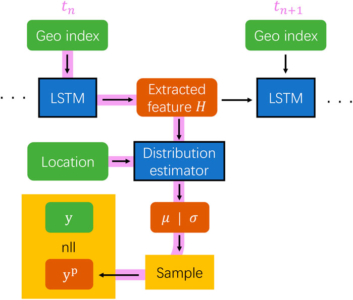
FIGURE 1. Model structure and workflow. Purple line: data flow at time $t_n$; Green box: model input; Blue box: neural network model modules; Red box: (intermediate) model output; Yellow box: data operation. After the hidden state $H$ is encoded by LSTM from the geomagnetic indices, a probability distribution is estimated at the satellite location, and a prediction $y^p$ is sampled from this distribution. The negative log likelihood (nll) is calculated between the prediction $y^p$ and satellite observation $y$, and is further used to update the model parameters through backpropagation. $y$ denotes either total electron density or hiss wave amplitude.

As hiss wave amplitude varies significantly in different regions, models tend to estimate the average activity while treating the variation as noise, thus underestimating the wave activity (trained with the same model structure as Huang et al. (2022) on hiss wave; not shown here). To better capture the dynamic nature of hiss wave activity, instead of directly predicting a quantity in a deterministic approach, we use a neural network module that estimates the wave probability distribution (modeling both the mean μ and standard deviation σ) at a specific location and time. This approach essentially introduces an estimation of the uncertainty (Blundell et al., 2015) in the data and is critical to model quantities with large variations (Tasistro-Hart et al., 2021). We avoid applying significant smoothing to the RBSP data to retain the full information carried in the variation. We sample a prediction $y^p$ from the modeled mean and standard deviation and calculate the negative log likelihood

$nll={\displaystyle \sum _i}\left(\log \sqrt{2\pi {\sigma }^2}+\frac{{\left(y_i-\mu \right)}^2}{2{\sigma }^2}\right)$

between the observation and model prediction. This process essentially maximizes the possibility of measuring the observed quantity given the estimated distribution. The calculated loss is then used to update the model parameters through the standard backpropagation procedure.

To address the issue of an unbalanced dataset in training the hiss wave model, we have implemented a weighted sampler. While we dedicate considerable attention to geomagnetically active times, it is important to note that quiet times are more common and generally exhibit low wave activities. When the model is trained on the entire dataset, it tends to learn more efficiently from weaker waves, resulting in an underestimation of wave activity. To mitigate this imbalance, we use a weighted sampler that selects training samples based on a probability proportional to the largest wave amplitude within the subsequent 1-h period. Consequently, periods with stronger wave activity are more likely to be included in the training process than those with weak wave activity, leading to a model with improved performance during geomagnetically active times.

We include more details of the model structure and optimization procedure in Appendix A.

2.4 Data processing

The data from 2013 to 2019 is divided into 7-day blocks, with 70% randomly assigned as the training set, 20% as the validation set, and 10% as the test set. The period 13–19 May 2019 is also kept in the test set for further simulation (see Section 3.2). This division into 7-day blocks is chosen to avoid data leakage that is common in time-series modeling, and is short enough to allow for a large number of blocks, and long enough to prevent information leakage, while also considering long-term seasonal and solar cycle variations. After the training time range is settled (7-day blocks that belong to the training set combined), during each runtime we generate training samples with a weighted sampler using the following procedure. 1) Before the training starts, both Van Allen Probe A and B observations that fall within these 7-day blocks are assigned with a sequence of weights. Each weight that corresponds to a certain timestamp is calculated to be proportional to the largest wave amplitude within the subsequent 1-h period. The resulting weight sequence has the same length as satellite observations. 2) During the training, starting times of the satellite observations are randomly picked given the weight sequence, and for each selected time, a period of 10-h that follows the selected time is used in the training process. Each 10-h period of observation is then paired with the corresponding 10 h of geomagnetic indicies and the preceding 24 h of historical geomagnetic indices at 1-min resolution to provide information on the state of the inner magnetosphere. In summary, for each 10-h period, the model takes 24 h of historical geomagnetic indices (consisting of 1,440 data points) as inputs, followed by another 10 h of geomagnetic indices (consisting of 600 data points) and satellite location (L, sin (MLT/12*π), cos (MLT/12*π), MLAT) at the same time. The model predicts the total electron density and hiss wave amplitude within the 10-h period. The negative log likelihood is calculated between observation and model prediction over each 10-h period. Loss is accumulated over a number of sequences trained at the same time, until it backpropagates to update the neural network parameters.

3 Results

3.1 Model performance

The overall model performance is shown in Figure 2 for total electron density (A-C) and hiss wave amplitude (D-F) for different datasets, respectively. The x-axis represents the observed quantity $y$ (density or hiss wave amplitude), while the y-axis represents the corresponding modeled quantity $y^p$. The color represents how many $\mathrm{y}-{\mathrm{y}}^{\mathrm{p}}$ pairs are located in that region. The red dashed diagonal line indicates a perfect model prediction ($\mathrm{y}={\mathrm{y}}^{\mathrm{p}}$). The darker areas, concentrated near the red line, indicate good model performance for the majority of the data. This is also quantified by the correlation coefficient between ${\log }_{10}y$ and ${\log }_{10}{y}^p$ denoted by “r” in each panel. The model performance for electron density is similar to that of Huang et al. (2022), where the Pearson correlation coefficient for the test dataset (Figure 2C) is about 0.9, close to that of the validation set (Figure 2B) indicating that the model generalization ability is good. The mean square error (MSE) and median error are 0.16 and 0.017, respectively. This indicates that the error is evenly distributed along the true values, signifying that the model both generalizes well and performs well in modeling electron density. For the hiss wave amplitude, there is more spread of the darker areas (Figure 2F) with r = 0.74, mse = 0.53 and median = −0.009 for the test dataset, which suggests that the model performance is worse for the hiss amplitude than electron density. This is partly because the wave activity is highly dynamic, exhibiting fluctuations on short timescales, and thus is less predictable compared to the cold plasma density. Nevertheless, by adopting a probability-based approach, our model reproduces the general global wave evolution fairly well, as presented in the following section.

FIGURE 2

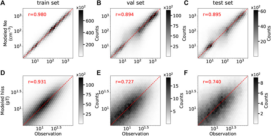
FIGURE 2. Overall model performance of electron density (A–C) and hiss wave amplitude (D–F) for different datasets. X-axis: observed quantity; Y-axis: modeled quantity. The correlation coefficient is calculated and labeled as “r.” The Red dashed line denotes the data pair where the model prediction matches the observed value perfectly.

3.2 Event study

We present a case study focusing on the global evolution of hiss waves and evaluate their effects on the energetic electron dynamics during a storm event on 14 May 2019, which is intentionally excluded from the training set. RBSP observations reveal the formation of a plasmaspheric plume and intensification of hiss waves over 13–19 May 2019, as shown in Figure 3. The SYM-H and SML indices (Figure 3A) peaked on May 14 when RBSP was on the dayside and observed a clear signature of the plasmaspheric plume (first by RBSP-A and later by RBSP-B, marked with black arrows in Figures 3B,C, respectively). Hiss wave amplitude intensified during the event (Figures 3D–H). show binned satellite observations of energetic electron fluxes at energies of 132 keV, 235 keV, and 470 keV, respectively. The electron flux increased by an order of magnitude from L∼ 5 to L∼3 within several hours during the main phase of the storm, which occurred at 7 UT on May 14. After the storm main phase, the electron flux decayed gradually over the subsequent days due to radial diffusion and pitch-angle scattering by waves that we will model later. We plot the modeled electron density and hiss wave amplitude in panels (B)–(E) and show a line-by-line comparison between the model (orange) and the observation (blue) during the event. Overall, the model accurately captures the evolution of the plasmapause location, especially during the latter half of the event when SYM-H and SML were very quiet while Kp varied. There were instances when RBSP measured very low density (<10 cm⁻³), but the model predicted slightly higher density (−30 cm⁻³). Although the relative error is significant, the absolute error remains relatively low. The modeled hiss wave amplitude generally follows the observations, successfully capturing most of the peak values.

FIGURE 3

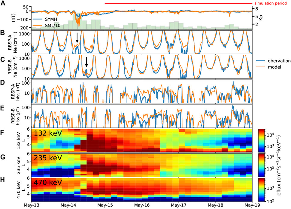
FIGURE 3. Overview of the geomagnetic storm during 13–19 May 2019. (A) SYM-H, SML, and Kp indices during the event. (B–C) Comparison between modeled electron density (orange) and satellite observation (blue) for RBSP-A and -B, respectively. Black arrows indicate plume features observed by the satellites. (D–E) Same as (B–C), but for hiss wave amplitude. (F–H) Measured spin-averaged electron flux at different energy channels.

Figure 4 provides several snapshots illustrating the modeled global evolution of both electron density and hiss waves, allowing for a more comprehensive understanding of their dynamics during and following the storm event. As indicated by SYM-H and SML in panel (A), we select six specific times (1-6) to examine the modeled electron density (B) and hiss wave amplitude (C) before, during, and after the storm. Before the storm onset (1), the plasmasphere was relatively quiet and extended up to L = 6 on the dusk side. Correspondingly, hiss wave activity was low, which is expected during quiet conditions (Li et al., 2015a; Kim et al., 2015). As the storm intensified (2) with higher Kp and decreased SYM-H, the plasmasphere was pushed to the dayside due to the enhanced convection electric field, and hiss waves were intensified in the dawn-to-noon sector, probably related to the enhanced injection from the nightside plasma sheet. As the storm progressed (3), the plasmaspheric plume was formed, and the region with strong hiss waves shifted to the dusk side. The intensified waves predominantly occurred at high L, showing a good spatial correlation with the plume, in agreement with the statistical results of plume hiss (Shi et al., 2019). During the recovery phase from (3) to (5), the model predicted a rotating and narrowing plume, consistent with physical simulation results (De Pascuale et al., 2018), with hiss waves rotating and decaying simultaneously. After the storm, instances of persistent moderate hiss wave activity were observed (6). During the entire period, the majority of the wave power was concentrated near the plasmapause, in agreement with statistical results (Malaspina et al., 2017).

FIGURE 4

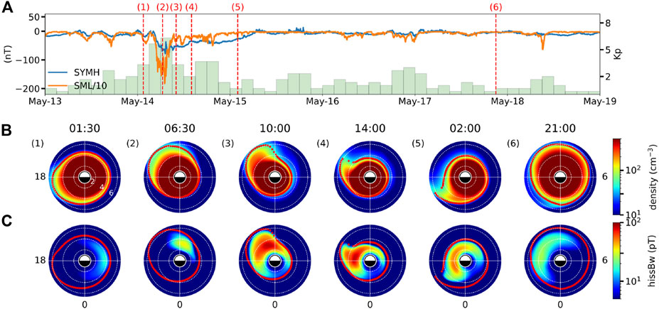
FIGURE 4. Snapshots of a geomagnetic storm event during 13–19 May 2019. (A) SYM-H, SML, and Kp indices during the event. (B) Modeled total electron density on the equatorial plane at different times, indicated by red dashed lines in panel (A). The contour of electron density of 50 cm^-3 is overplotted as a red line to indicate the plasmapause. White dashed circles represent L = 2, 4, and 6. (C) Same as panel (B), but for hiss wave amplitude.

3.3 Event simulation

We use the UCLA 3-D diffusion code (Ma et al., 2015; 2018) to simulate the energetic electron evolution, considering radial diffusion and local resonant interactions with hiss waves. The simulation starts at 00 UT on May 15, following a period of significant local electron acceleration period and the extension of the plasmapause beyond L = 4. During the following four quiet days, the electron flux gradually decayed, providing a unique opportunity to model the effects of pitch angle scattering caused by hiss waves. The observed electron fluxes at 00 UT on May 15 are used as the initial condition for all L shells, as well as the time-varying boundary conditions at L = 2.6 and L = 6. The energy range in the simulation is set from 374 keV to 4.5 MeV at L = 2.6 and from 40 keV to 1 MeV at L = 6, maintaining the conservation of the first adiabatic invariant. The pitch angle gradients of phase space density at α = 0° and α = 90° are set to be 0. The modeling results of energetic electron fluxes are not sensitive to the energy boundary condition assumptions because the energy diffusion coefficients due to hiss are much smaller than the pitch angle diffusion coefficients (e.g., Ni et al., 2013; Thorne et al., 2013). Radial diffusion coefficients are calculated using the formulation by Liu et al. (2016) with pitch angle dependence from Schulz (1991, p229). The pitch angle, momentum, and their mixed diffusion coefficients are computed based on the total plasma density and hiss wave amplitude obtained from the deep learning model with a time cadence of 5 min. The wave frequency spectrum is derived from the Van Allen Probes statistics (Li et al., 2015b), and wave normal angles are assumed to be quasi field-aligned near the magnetic equator, gradually becoming highly oblique at higher latitudes (Ni et al., 2013). The deep learning model provides the time-varying total electron density and hiss wave amplitude as functions of L shell and MLT at the equator, which are used as inputs to the 3-D diffusion code.

Figure 5 shows the modeled MLT-averaged hiss wave amplitude (A) and the simulated energetic electron flux evolution (B-D) in the same energy channels as shown in Figure 3. At the start of the simulation on May 15, the energetic electron fluxes were initially high in the outer radiation belt. As a result of both radial diffusion and scattering by hiss waves, the electron flux gradually decayed over the following 1–3 days. Instances of faster decay and slumps in the electron flux were successfully reproduced by the simulation at 0 and 18 UT on May 17, consistent with the RBSP observations. These slumps can be attributed to the enhanced wave activity, which causes stronger pitch angle scattering. To quantify the role of plume hiss in energetic electron dynamics, we divided the modeled global distribution of hiss waves into plume hiss and plasmaspheric hiss based on the modeled total electron density. We defined the plume as the region with a total electron density in the range 20–200 cm⁻³, as identified from the global maps of modeled electron density, in agreement with typical plume statistics (Moldwin, 2004; Darrouzet et al., 2008). Although this definition may include the outer plasmasphere, as well as attached or detached plumes, it serves our purpose as this region exhibits similar characteristics that allow access for energetic electrons, potentially providing a source of free energy for whistler mode wave intensification (e.g., Li et al., 2013; Shi et al., 2019). Figure 5E displays the modeled plume hiss, characterized by an MLT-averaged wave amplitude of ∼10–20 pT. The majority of the plume hiss was located at L ∼ 5, although the coverage was sometimes extended to L > 6. Despite its high variability, a clear trend emerged during the first 3 days, indicating that the inner edge of the plume hiss moved from L = 4 to 5 due to the refilling of the plasmasphere after the storm.

FIGURE 5

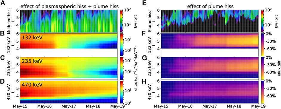
FIGURE 5. Simulated energetic flux evolution during a quiet period. (A) MLT-averaged hiss wave amplitude as a function of L and time from the deep learning model. (B) Simulated electron flux evolution for 132 keV electrons as a function of L and time, starting at L > 4. (C) Same as panel (B) but for 235 keV electrons. (D) Same as panel (B) but for 470 keV electrons. (E) Modeled MLT-averaged plume hiss wave amplitude. (F) Difference in simulated electron flux with and without plume hiss for 132 keV electrons. (G) Same as panel (F) but for 235 keV electrons. (H) Same as panel (F) but for 470 keV electrons.

To assess the impact of plume hiss on energetic electron flux, we conducted simulations considering only plasmaspheric hiss and compared them with simulations that included the effects of both plasmaspheric and plume hiss (the simulated electron fluxes are denoted as $J_1$ and $J_2$, respectively). The difference in electron fluxes between these simulations, quantified by $\left(J_1-J_2\right)/J_1$, represents the sole effect of plume hiss, as shown in panels (F-H). When the plume hiss effect was included, there was a consistent decrease in electron fluxes over the 100–500 keV energy range. After a few days of simulation, the plume hiss accounted for an −80% decrease in 132 keV electron flux and a −40% decrease in 470 keV electron flux at L−4.5, near the heart of the outer radiation belt. At higher L, the plume hiss also contributed significantly to electron losses, resulting in a −30%–70% decrease in electron flux at L−5.5. It is worth noting that the hiss wave activity depicted in Figure 5A is relatively modest, but the peak wave amplitude reached up to −100 pT. The averaged value of hiss wave amplitude during the recovery phase of this event is lower than the averaged statistical wave amplitude (−100 pT) on the dayside during strong geomagnetic conditions with AL* < −500 nT (Li et al., 2015a). It is interesting to note that there have been instances where hiss wave amplitudes in plumes exceeded 1,000 pT (Su et al., 2018). Therefore, we expect that plume hiss waves would have a much stronger impact during periods of higher geomagnetic activity.

Figure 6 presents a comparison between the simulated (dashed line) and the observed electron flux evolution (solid line) at L = 4.4. This L shell is located in the heart of the outer radiation belt, where the electron flux decay is most prominent. Moreover, choosing L = 4.4 ensures that it is sufficiently distant from the simulation boundary, thus the change at this distance is mostly from the simulation itself, minimizing the potential impact of using observations as boundary conditions. In all three energy channels, the simulation exhibits a gradual flux decay from May 15 to 16, followed by a faster decay from 16 to 17. The simulation accurately captures the electron flux decay rate until the end of May 18, when the observation reveals a faster decay of higher-energy electrons. This faster decay could be attributed to the influence of waves other than hiss waves alone, as discussed below.

FIGURE 6

FIGURE 6. Comparison between the simulated (dashed line) and the observed electron flux evolution (solid line) at L = 4.4. Each color represents a different energy channel.

4 Discussion

Although the simulated electron flux reproduced the observed flux for most of the period, there was a slightly faster decay rate in the observed flux on the last day of the simulation. Several potential factors could contribute to this discrepancy, which are discussed below.

1. The presence of waves other than hiss waves can affect energetic electron dynamics. For example, chorus waves can also scatter electrons in the energy range of hundreds of keV, especially on the nightside where the plasmapause is often located at L < −5. When performing simulations that include both chorus and hiss waves, the effects of these waves will be taken into consideration. However, this is beyond the scope of the present study, as we focus solely on modeling the hiss wave distribution in the plasmasphere and plume and their quantitative scattering effects on electrons.

2. The presence of other waves may not scatter particles directly, but instead enhance the efficiency of hiss waves in scattering energetic electrons into the loss cone. Previous studies have shown that when electromagnetic ion cyclotron (EMIC) waves and hiss waves coexist at the same L shell, MeV electrons can be first scattered by hiss waves and subsequently scattered and precipitated by EMIC waves (Ma et al., 2015; Drozdov et al., 2020), resulting in a significant reduction in their lifetimes (Li et al., 2007; Zhang et al., 2017). Fast magnetosonic waves can induce additional scattering at intermediate pitch angles, leading to increased electron losses compared to scattering by hiss alone (Hua et al., 2018). Non-linear phase trapping by chorus waves can accelerate 300–500 keV electrons, which may then resonate with EMIC waves, resulting in their rapid scattering into the loss cone (Bashir et al., 2022). The combined effects of different wave modes on the radiation belt dynamics are beyond the scope of the present study and are left for future investigations.

There are different ways to define plumes used in simulations. In our study, we define the plume region as an area with a total electron density ranging from 20 to 200 cm^-3 at L < 6. This definition typically encompasses the outer plasmasphere or the plume, where energetic electrons (>−10s keV) can access, thus leading to highly variable wave activity over time and space. We have found a considerable amount of hiss wave power at L > 4, and the outermost extension of hiss waves has been observed to vary from L = 4 to 6, even during relatively quiet periods indicated by the geomagnetic indices. The commonly used density and wave statistical models, which are often expressed as simple functions of Kp and/or AE (O’Brien and Moldwin, 2003; Golden et al., 2012; Spasojevic et al., 2015; Saikin et al., 2022), do not capture such variability since the underlying geomagnetic indices might not exhibit strong variations during the period. These statistical models predict a constant wave power at a given location for a range of geomagnetic indices. Our findings demonstrate that even under relatively quiet conditions, hiss wave activity could exhibit dynamic evolution, and such spatial variation plays a crucial role in the evolution of energetic electron fluxes over time at different L shells, as shown in Figure 5.

5 Conclusion

We have developed a neural network model to simultaneously reconstruct the global evolution of both electron density and hiss wave amplitude in the Earth’s plasmasphere and plume. Unlike traditional deterministic models, our approach estimates the distribution of these quantities, allowing for a better representation of variations in the data on both large and small scales.

To quantify the evolution and effects of plume hiss, we focused on the storm event that occurred over 13–19 May 2019, during which RBSP observed the formation of a plasmaspheric plume, followed by a gradual decay in the electron fluxes at a few hundred keV. Our model successfully captured the global evolution of the plume, as well as the plume hiss within it during the entire event. As geomagnetic activity increased, hiss wave power intensified and shifted from dawn to dusk, where the plume was formed later. The plume and plume hiss exhibited a strong spatial correlation and rotated together as the geomagnetic activity became weaker. The plume wrapped around the Earth and became thinner over the nightside, where hiss wave power diminished rapidly. During the recovery phase, the plasmasphere was gradually refilled, and hiss wave activity remained relatively low in general. Our model provided valuable insights into the relationship between the plume structure (as seen in the plasma density) and plume hiss on a global scale.

To quantify the impact of plume hiss, we separated the modeled total hiss wave population into plasmaspheric hiss and plume hiss, and simulated the energetic electron flux evolution with and without plume hiss. By including both plasmaspheric and plume hiss, together with radial diffusion, the simulated electron flux decay reproduces the observation very well. The remaining differences in the electron flux decay may be attributed to scattering effects from other waves. Although the MLT-averaged wave amplitude was −10–20 pT, plume hiss alone was responsible for an additional −80% decrease in 132 keV electron flux at L−4.5 within 3 days, and −30% decrease in 470 keV electron flux at L−5.5. These results highlight the dynamic nature of hiss wave evolution even during geomagnetically quiet conditions, and emphasize the significant role played by plume hiss in shaping the energetic electron dynamics, especially in the outer radiation belt, which should be considered in future simulations of radiation belt dynamics.

Data availability statement

The datasets presented in this study can be found in online repositories. The names of the repository/repositories and accession number(s) can be found below: The Van Allen Probes data from the EMFISIS instrument were obtained from http://emfisis.physics.uiowa.edu/Flight/. Data from the ECT instrument were obtained from https://rbsp-ect.newmexicoconsortium.org/data_pub/. The geomagnetic indices used in the model training are available at https://omniweb.gsfc.nasa.gov/form/omni_min.html (SYM-H); https://supermag.jhuapl.edu (SML and SMU); https://www.gfz-potsdam.de/en/hpo-index/ (Hp30). All data used to produce figures, as well as the Python script defining the model structure, are publicly available at https://doi.org/10.6084/m9.figshare.22817531.

Author contributions

SH and WL developed the study concept and lead the project. SH designed, implemented, and trained the neural network model, and performed the event analysis. QM performed the Fokker-Planck simulation and produced Figure 5. X-CS processed the wave spectrum data from EMFISIS and generated the dataset of hiss. LC contributed to the model design and event analysis. XC, DM, JB, MH, and SW contributed to the model design. SH wrote the first draft of the manuscript. All authors contributed to the article and approved the submitted version.

Funding

This research at Boston University is supported by the NASA Grants 80NSSC19K0845, 80NSSC20K0196, 80NSSC20K0704, and 80NSSC21K1312, and the NSF Grants AGS-1847818 and AGS-2225445. SH gratefully acknowledges the NASA FINESST Grant 80NSSC21K1385. SW acknowledges the support of NASA Grant 80NSSC20K0704. JB and DM gratefully acknowledge support from subgrant No. 1559841 to the University of California, Los Angeles, from the University of Colorado Boulder under NASA Prime Grant agreement No. 80NSSC20K1580.

Acknowledgments

We gratefully acknowledge the Van Allen Probes Mission, especially EMFISIS and ECT teams, for the use of their data. We also acknowledge the OMNI team, SuperMAG collaborators, GFZ collaborators, and the PyTorch team.

Conflict of interest

The authors declare that the research was conducted in the absence of any commercial or financial relationships that could be construed as a potential conflict of interest.

Publisher’s note

All claims expressed in this article are solely those of the authors and do not necessarily represent those of their affiliated organizations, or those of the publisher, the editors and the reviewers. Any product that may be evaluated in this article, or claim that may be made by its manufacturer, is not guaranteed or endorsed by the publisher.

References

Agapitov, O., Mourenas, D., Artemyev, A., Mozer, F. S., Bonnell, J. W., Angelopoulos, V., et al. (2018). Spatial extent and temporal correlation of chorus and hiss: statistical results from multipoint themis observations. J. Geophys. Res. Space Phys. 123 (10), 8317–8330. doi:10.1029/2018JA025725

CrossRef Full Text | Google Scholar

Bashir, M. F., Artemyev, A., Zhang, X., and Angelopoulos, V. (2022). Energetic electron precipitation driven by the combined effect of ULF, EMIC, and whistler waves. J. Geophys. Res. Space Phys. 127 (1). doi:10.1029/2021JA029871

CrossRef Full Text | Google Scholar

Blake, J. B., Carranza, P. A., Claudepierre, S. G., Clemmons, J. H., Crain, W. R., Dotan, Y., et al. (2013). The magnetic electron ion spectrometer (MagEIS) instruments aboard the radiation belt storm probes (RBSP) spacecraft. Space Sci. Rev. 179 (1–4), 383–421. doi:10.1007/s11214-013-9991-8

CrossRef Full Text | Google Scholar

Blundell, C., Cornebise, J., Kavukcuoglu, K., and Wierstra, D. (2015). Weight uncertainty in neural networks. Retrieved from http://arxiv.org/abs/1505.05424.

Google Scholar

Bortnik, Jacob, Thorne, R. M., and Meredith, N. P. (2009b). Plasmaspheric hiss overview and relation to chorus. J. Atmos. Solar-Terrestrial Phys. 71 (16), 1636–1646. doi:10.1016/j.jastp.2009.03.023

CrossRef Full Text | Google Scholar

Bortnik, J. (2003). Frequency-time spectra of magnetospherically reflecting whistlers in the plasmasphere. J. Geophys. Res. 108 (A1), 1030. doi:10.1029/2002JA009387

CrossRef Full Text | Google Scholar

Bortnik, J., Li, W., Thorne, R. M., Angelopoulos, V., Cully, C., Bonnell, J., et al. (2009a). An observation linking the origin of plasmaspheric hiss to discrete chorus emissions. Science 324 (5928), 775–778. doi:10.1126/science.1171273

PubMed Abstract | CrossRef Full Text | Google Scholar

Bortnik, J., Thorne, R. M., and Meredith, N. P. (2008). The unexpected origin of plasmaspheric hiss from discrete chorus emissions. Nature 452 (7183), 62–66. doi:10.1038/nature06741

PubMed Abstract | CrossRef Full Text | Google Scholar

Chan, K.-W., and Holzer, R. E. (1976). ELF hiss associated with plasma density enhancements in the outer magnetosphere. J. Geophys. Res. 81 (13), 2267–2274. doi:10.1029/JA081i013p02267

CrossRef Full Text | Google Scholar

Chen, L., Bortnik, J., Li, W., Thorne, R. M., and Horne, R. B. (2012a). Modeling the properties of plasmaspheric hiss: 1. Dependence on chorus wave emission. J. Geophys. Res. Space Phys. 117 (A5). doi:10.1029/2011JA017201

CrossRef Full Text | Google Scholar

Chen, L., Bortnik, J., Li, W., Thorne, R. M., and Horne, R. B. (2012b). Modeling the properties of plasmaspheric hiss: 2. Dependence on the plasma density distribution. J. Geophys. Res. Space Phys. 117 (A5). doi:10.1029/2011JA017202

CrossRef Full Text | Google Scholar

Chen, L., Thorne, R. M., Bortnik, J., Li, W., Horne, R. B., Reeves, G. D., et al. (2014). Generation of unusually low frequency plasmaspheric hiss. Geophys. Res. Lett. 41 (16), 5702–5709. doi:10.1002/2014GL060628

CrossRef Full Text | Google Scholar

Church, S. R., and Thorne, R. M. (1983). On the origin of plasmaspheric hiss: ray path integrated amplification. J. Geophys. Res. 88 (A10), 7941. doi:10.1029/JA088iA10p07941

CrossRef Full Text | Google Scholar

Darrouzet, F., De Keyser, J., Décréau, P. M. E., El Lemdani-Mazouz, F., and Vallières, X. (2008). Statistical analysis of plasmaspheric plumes with Cluster/WHISPER observations. Ann. Geophys. 26 (8), 2403–2417. doi:10.5194/angeo-26-2403-2008

CrossRef Full Text | Google Scholar

De Pascuale, S., Jordanova, V. K., Goldstein, J., Kletzing, C. A., Kurth, W. S., Thaller, S. A., et al. (2018). Simulations of van allen probes plasmaspheric electron density observations. J. Geophys. Res. Space Phys. 123 (11), 9453–9475. doi:10.1029/2018JA025776

CrossRef Full Text | Google Scholar

Drozdov, A. Y., Usanova, M. E., Hudson, M. K., Allison, H. J., and Shprits, Y. Y. (2020). The role of hiss, chorus, and EMIC waves in the modeling of the dynamics of the multi-MeV radiation belt electrons. J. Geophys. Res. Space Phys. 125 (9). doi:10.1029/2020JA028282

CrossRef Full Text | Google Scholar

Dunckel, N., and Helliwell, R. A. (1969). Whistler-mode emissions on the OGO 1 satellite. J. Geophys. Res. 74 (26), 6371–6385. doi:10.1029/JA074i026p06371

CrossRef Full Text | Google Scholar

Fu, H., Yue, C., Ma, Q., Kang, N., Bortnik, J., Zong, Q., et al. (2021). Frequency-dependent responses of plasmaspheric hiss to the impact of an interplanetary shock. Geophys. Res. Lett. 48 (20). doi:10.1029/2021GL094810

CrossRef Full Text | Google Scholar

Gjerloev, J. W. (2012). The SuperMAG data processing technique: technique. J. Geophys. Res. Space Phys. 117 (A9). doi:10.1029/2012JA017683

CrossRef Full Text | Google Scholar

Golden, D. I., Spasojevic, M., Li, W., and Nishimura, Y. (2012). Statistical modeling of plasmaspheric hiss amplitude using solar wind measurements and geomagnetic indices: modeling HISS with solar wind. Geophys. Res. Lett. 39 (6). doi:10.1029/2012GL051185

CrossRef Full Text | Google Scholar

Green, J. L. (2005). On the origin of whistler mode radiation in the plasmasphere. J. Geophys. Res. 110 (A3), A03201. doi:10.1029/2004JA010495

CrossRef Full Text | Google Scholar

Hayakawa, M., and Sazhin, S. S. (1992). Mid-latitude and plasmaspheric hiss: A review. Planet. Space Sci. 40 (10), 1325–1338. doi:10.1016/0032-0633(92)90089-7

CrossRef Full Text | Google Scholar

Hayakawa, M., Ohmi, N., Parrot, M., and Lefeuvre, F. (1986). Direction finding of ELF hiss emissions in a detached plasma region of the magnetosphere. J. Geophys. Res. 91 (A1), 135. doi:10.1029/JA091iA01p00135

CrossRef Full Text | Google Scholar

Hochreiter, S., and Schmidhuber, J. (1997). Long short-term memory. Neural Comput. 9 (8), 1735–1780. doi:10.1162/neco.1997.9.8.1735

PubMed Abstract | CrossRef Full Text | Google Scholar

Horne, R. B., and Thorne, R. M. (1998). Potential waves for relativistic electron scattering and stochastic acceleration during magnetic storms. Geophys. Res. Lett. 25 (15), 3011–3014. doi:10.1029/98GL01002

CrossRef Full Text | Google Scholar

Hua, M., Ni, B., Fu, S., Gu, X., Xiang, Z., Cao, X., et al. (2018). Combined scattering of outer radiation belt electrons by simultaneously occurring chorus, exohiss, and magnetosonic waves. Geophys. Res. Lett. 45 (19). doi:10.1029/2018GL079533

CrossRef Full Text | Google Scholar

Huang, C. Y., Goertz, C. K., and Anderson, R. R. (1983). A theoretical study of plasmaspheric hiss generation. J. Geophys. Res. 88 (A10), 7927. doi:10.1029/JA088iA10p07927

CrossRef Full Text | Google Scholar

Huang, S., Li, W., Shen, X., Ma, Q., Chu, X., Ma, D., et al. (2022). Application of recurrent neural network to modeling Earth’s global electron density. J. Geophys. Res. Space Phys. 127 (9). doi:10.1029/2022JA030695

CrossRef Full Text | Google Scholar

Karim, F., Majumdar, S., Darabi, H., and Chen, S. (2018). LSTM fully convolutional networks for time series classification. IEEE Access 6, 1662–1669. doi:10.1109/ACCESS.2017.2779939

CrossRef Full Text | Google Scholar

Kennel, C. F., and Petschek, H. E. (1966). Limit on stably trapped particle fluxes. J. Geophys. Res. 71 (1), 1–28. doi:10.1029/JZ071i001p00001

CrossRef Full Text | Google Scholar

Kim, K., Lee, D., and Shprits, Y. (2015). Dependence of plasmaspheric hiss on solar wind parameters and geomagnetic activity and modeling of its global distribution. J. Geophys. Res. Space Phys. 120 (2), 1153–1167. doi:10.1002/2014JA020687

CrossRef Full Text | Google Scholar

Kletzing, C. A., Kurth, W. S., Acuna, M., MacDowall, R. J., Torbert, R. B., Averkamp, T., et al. (2013). The electric and magnetic field instrument suite and integrated science (EMFISIS) on RBSP. Space Sci. Rev. 179 (1–4), 127–181. doi:10.1007/s11214-013-9993-6

CrossRef Full Text | Google Scholar

Kurth, W. S., De Pascuale, S., Faden, J. B., Kletzing, C. A., Hospodarsky, G. B., Thaller, S., et al. (2015). Electron densities inferred from plasma wave spectra obtained by the Waves instrument on Van Allen Probes. J. Geophys. Res. Space Phys. 120 (2), 904–914. doi:10.1002/2014JA020857

PubMed Abstract | CrossRef Full Text | Google Scholar

Lam, M. M., Horne, R. B., Meredith, N. P., and Glauert, S. A. (2007). Modeling the effects of radial diffusion and plasmaspheric hiss on outer radiation belt electrons. Geophys. Res. Lett. 34 (20), L20112. doi:10.1029/2007GL031598

CrossRef Full Text | Google Scholar

Larkina, V. I., and Likhter, Ja. I. (1982). Storm-time variations of plasmaspheric ELF hiss. J. Atmos. Terr. Phys. 44 (5), 415–423. doi:10.1016/0021-9169(82)90048-4

CrossRef Full Text | Google Scholar

Li, W., Chen, L., Bortnik, J., Thorne, R. M., Angelopoulos, V., Kletzing, C. A., et al. (2015b). First evidence for chorus at a large geocentric distance as a source of plasmaspheric hiss: coordinated themis and van allen probes observation. Geophys. Res. Lett. 42 (2), 241–248. doi:10.1002/2014GL062832

CrossRef Full Text | Google Scholar

Li, W., Ma, Q., Thorne, R. M., Bortnik, J., Kletzing, C. A., Kurth, W. S., et al. (2015a). Statistical properties of plasmaspheric hiss derived from Van Allen Probes data and their effects on radiation belt electron dynamics. J. Geophys. Res. Space Phys. 120 (5), 3393–3405. doi:10.1002/2015JA021048

CrossRef Full Text | Google Scholar

Li, W., Shen, X. -C., Ma, Q., Capannolo, L., Shi, R., Redmon, R. J., et al. (2019). Quantification of energetic electron precipitation driven by plume whistler mode waves, plasmaspheric hiss, and exohiss. Geophys. Res. Lett. 46 (7), 3615–3624. doi:10.1029/2019GL082095

CrossRef Full Text | Google Scholar

Li, W., Shprits, Y. Y., and Thorne, R. M. (2007). Dynamic evolution of energetic outer zone electrons due to wave-particle interactions during storms. J. Geophys. Res. Space Phys. 112 (A10). doi:10.1029/2007JA012368

CrossRef Full Text | Google Scholar

Li, W., Thorne, R. M., Bortnik, J., Reeves, G. D., Kletzing, C. A., Kurth, W. S., et al. (2013). An unusual enhancement of low-frequency plasmaspheric hiss in the outer plasmasphere associated with substorm-injected electrons: amplification of low-frequency HISS. Geophys. Res. Lett. 40 (15), 3798–3803. doi:10.1002/grl.50787

CrossRef Full Text | Google Scholar

Liu, N., Su, Z., Gao, Z., Zheng, H., Wang, Y., Wang, S., et al. (2020). Comprehensive observations of substorm-enhanced plasmaspheric hiss generation, propagation, and dissipation. Geophys. Res. Lett. 47 (2). doi:10.1029/2019GL086040

CrossRef Full Text | Google Scholar

Liu, W., Tu, W., Li, X., Sarris, T., Khotyaintsev, Y., Fu, H., et al. (2016). On the calculation of electric diffusion coefficient of radiation belt electrons with in situ electric field measurements by THEMIS. Geophys. Res. Lett. 43 (3), 1023–1030. doi:10.1002/2015GL067398

CrossRef Full Text | Google Scholar

Ma, Q., Li, W., Bortnik, J., Thorne, R. M., Chu, X., Ozeke, L. G., et al. (2018). Quantitative evaluation of radial diffusion and local acceleration processes during GEM challenge events. J. Geophys. Res. Space Phys. 123 (3), 1938–1952. doi:10.1002/2017JA025114

CrossRef Full Text | Google Scholar

Ma, Q., Li, W., Thorne, R. M., Bortnik, J., Reeves, G. D., Kletzing, C. A., et al. (2016). Characteristic energy range of electron scattering due to plasmaspheric hiss. J. Geophys. Res. Space Phys. 121 (12). doi:10.1002/2016JA023311

CrossRef Full Text | Google Scholar

Ma, Q., Li, W., Thorne, R. M., Ni, B., Kletzing, C. A., Kurth, W. S., et al. (2015). Modeling inward diffusion and slow decay of energetic electrons in the Earth’s outer radiation belt. Geophys. Res. Lett. 42 (4), 987–995. doi:10.1002/2014GL062977

CrossRef Full Text | Google Scholar

Ma, Q., Li, W., Zhang, X. J., Bortnik, J., Shen, X. -C., Connor, H. K., et al. (2021). Global survey of electron precipitation due to hiss waves in the Earth’s plasmasphere and plumes. J. Geophys. Res. Space Phys. 126 (8). doi:10.1029/2021JA029644

CrossRef Full Text | Google Scholar

Malaspina, D. M., Jaynes, A. N., Hospodarsky, G., Bortnik, J., Ergun, R. E., and Wygant, J. (2017). Statistical properties of low-frequency plasmaspheric hiss. J. Geophys. Res. Space Phys. 122 (8), 8340–8352. doi:10.1002/2017JA024328

CrossRef Full Text | Google Scholar

Matzka, J., Stolle, C., Yamazaki, Y., Bronkalla, O., and Morschhauser, A. (2021). The geomagnetic kp index and derived indices of geomagnetic activity. Space weather. 19 (5). doi:10.1029/2020SW002641

CrossRef Full Text | Google Scholar

Mauk, B. H., Fox, N. J., Kanekal, S. G., Kessel, R. L., Sibeck, D. G., and Ukhorskiy, A. (2013). Science objectives and rationale for the radiation belt storm probes mission. Space Sci. Rev. 179 (1–4), 3–27. doi:10.1007/s11214-012-9908-y

CrossRef Full Text | Google Scholar

Meredith, N. P., Bortnik, J., Horne, R. B., Li, W., and Shen, X. (2021). Statistical investigation of the frequency dependence of the chorus source mechanism of plasmaspheric hiss. Geophys. Res. Lett. 48 (6). doi:10.1029/2021GL092725

CrossRef Full Text | Google Scholar

Meredith, N. P., Horne, R. B., Bortnik, J., Thorne, R. M., Chen, L., Li, W., et al. (2013). Global statistical evidence for chorus as the embryonic source of plasmaspheric hiss. Geophys. Res. Lett. 40 (12), 2891–2896. doi:10.1002/grl.50593

CrossRef Full Text | Google Scholar

Meredith, N. P., Horne, R. B., Clilverd, M. A., Horsfall, D., Thorne, R. M., and Anderson, R. R. (2006). Origins of plasmaspheric hiss. J. Geophys. Res. 111 (A9), A09217. doi:10.1029/2006JA011707

CrossRef Full Text | Google Scholar

Meredith, N. P. (2004). Substorm dependence of plasmaspheric hiss. J. Geophys. Res. 109 (A6), A06209. doi:10.1029/2004JA010387

CrossRef Full Text | Google Scholar

Millan, R. M., Ripoll, J.-F., Santolík, O., and Kurth, W. S. (2021). Early-time non-equilibrium pitch angle diffusion of electrons by whistler-mode hiss in a plasmaspheric plume associated with BARREL precipitation. Front. Astronomy Space Sci. 8, 776992. doi:10.3389/fspas.2021.776992

CrossRef Full Text | Google Scholar

Moldwin, M. B. (2004). Plasmaspheric plumes: CRRES observations of enhanced density beyond the plasmapause. J. Geophys. Res. 109 (A5), A05202. doi:10.1029/2003JA010320

CrossRef Full Text | Google Scholar

Newell, P. T., and Gjerloev, J. W. (2011). Evaluation of SuperMAG auroral electrojet indices as indicators of substorms and auroral power: supermag auroral electrojet indices. J. Geophys. Res. Space Phys. 116 (A12). doi:10.1029/2011JA016779

CrossRef Full Text | Google Scholar

Ni, B., Bortnik, J., Thorne, R. M., Ma, Q., and Chen, L. (2013). Resonant scattering and resultant pitch angle evolution of relativistic electrons by plasmaspheric hiss. J. Geophys. Res. Space Phys. 118 (12), 7740–7751. doi:10.1002/2013JA019260

CrossRef Full Text | Google Scholar

Ni, B., Li, W., Thorne, R. M., Bortnik, J., Ma, Q., Chen, L., et al. (2014). Resonant scattering of energetic electrons by unusual low-frequency hiss. Geophys. Res. Lett. 41 (6), 1854–1861. doi:10.1002/2014GL059389

CrossRef Full Text | Google Scholar

O’Brien, T. P., and Moldwin, M. B. (2003). Empirical plasmapause models from magnetic indices. Geophys. Res. Lett. 30 (4), 2002GL016007. doi:10.1029/2002GL016007

CrossRef Full Text | Google Scholar

Qin, M., Li, W., Ma, Q., Woodger, L., Millan, R., Shen, X., et al. (2021). Multi-point observations of modulated whistler-mode waves and energetic electron precipitation. J. Geophys. Res. Space Phys. 126 (12). doi:10.1029/2021JA029505

CrossRef Full Text | Google Scholar

Ripoll, J.-F., Denton, M., Loridan, V., Santolík, O., Malaspina, D., Hartley, D. P., et al. (2020). How whistler mode hiss waves and the plasmasphere drive the quiet decay of radiation belts electrons following a geomagnetic storm. J. Phys. Conf. Ser. 1623, 012005. doi:10.1088/1742-6596/1623/1/012005

CrossRef Full Text | Google Scholar

Russell, C. T., Holzer, R. E., and Smith, E. J. (1969). OGO 3 observations of ELF noise in the magnetosphere: 1. Spatial extent and frequency of occurrence. J. Geophys. Res. 74 (3), 755–777. doi:10.1029/JA074i003p00755

CrossRef Full Text | Google Scholar

Saikin, A. A., Drozdov, A. Y., and Malaspina, D. M. (2022). Low frequency plasmaspheric hiss wave activity parameterized by plasmapause location: models and simulations. J. Geophys. Res. Space Phys. 127 (9). doi:10.1029/2022JA030687

CrossRef Full Text | Google Scholar

Santolík, O., Chum, J., Parrot, M., Gurnett, D. A., Pickett, J. S., and Cornilleau-Wehrlin, N. (2006). Propagation of whistler mode chorus to low altitudes: spacecraft observations of structured elf hiss. J. Geophys. Res. 111 (A10), A10208. doi:10.1029/2005JA011462

CrossRef Full Text | Google Scholar

Schulz, M. (1991). “The magnetosphere,” in Geomagnetism (Elsevier), Amsterdam, Netherlands 87–293. doi:10.1016/B978-0-12-378674-6.50008-X

CrossRef Full Text | Google Scholar

Shen, X., Li, W., Ma, Q., Agapitov, O., and Nishimura, Y. (2019). Statistical analysis of transverse size of lower band chorus waves using simultaneous multisatellite observations. Geophys. Res. Lett. 46 (11), 5725–5734. doi:10.1029/2019GL083118

CrossRef Full Text | Google Scholar

Shi, R., Li, W., Ma, Q., Green, A., Kletzing, C. A., Kurth, W. S., et al. (2019). Properties of whistler mode waves in Earth’s plasmasphere and plumes. J. Geophys. Res. Space Phys. 124 (2), 1035–1051. doi:10.1029/2018JA026041

CrossRef Full Text | Google Scholar

Siami-Namini, S., Tavakoli, N., and Namin, A. S. (2019). The performance of LSTM and BiLSTM in forecasting time series. In Proceedings of the 2019 IEEE International Conference on Big Data (Big Data). Los Angeles, CA, USA.doi:10.1109/BigData47090.2019.9005997

CrossRef Full Text | Google Scholar

Sonwalkar, V. S., and Inan, U. S. (1989). Lightning as an embryonic source of VLF hiss. J. Geophys. Res. Space Phys. 94 (A6), 6986–6994. doi:10.1029/JA094iA06p06986

CrossRef Full Text | Google Scholar

Spasojevic, M., Shprits, Y. Y., and Orlova, K. (2015). Global empirical models of plasmaspheric hiss using Van Allen Probes. J. Geophys. Res. Space Phys. 120 (12). doi:10.1002/2015JA021803

CrossRef Full Text | Google Scholar

Spence, H. E., Reeves, G. D., Baker, D. N., Blake, J. B., Bolton, M., Bourdarie, S., et al. (2013). Science goals and overview of the radiation belt storm probes (RBSP) energetic particle, composition, and thermal plasma (ECT) suite on NASA’s van allen probes mission. Space Sci. Rev. 179 (1–4), 311–336. doi:10.1007/s11214-013-0007-5

CrossRef Full Text | Google Scholar

Su, Z., Liu, N., Zheng, H., Wang, Y., and Wang, S. (2018). Multipoint observations of nightside plasmaspheric hiss generated by substorm-injected electrons. Geophys. Res. Lett. 45 (20). doi:10.1029/2018GL079927

CrossRef Full Text | Google Scholar

Summers, D., Ni, B., Meredith, N. P., Horne, R. B., Thorne, R. M., Moldwin, M. B., et al. (2008). Electron scattering by whistler-mode ELF hiss in plasmaspheric plumes. J. Geophys. Res. 17. doi:10.1029/2007JA012678

CrossRef Full Text | Google Scholar

Tasistro-Hart, A., Grayver, A., and Kuvshinov, A. (2021). Probabilistic geomagnetic storm forecasting via deep learning. J. Geophys. Res. Space Phys. 126 (1). doi:10.1029/2020JA028228

CrossRef Full Text | Google Scholar

Thorne, Richard M., Smith, E. J., Burton, R. K., and Holzer, R. E. (1973). Plasmaspheric hiss. J. Geophys. Res. 78 (10), 1581–1596. doi:10.1029/JA078i010p01581

CrossRef Full Text | Google Scholar

Thorne, R. M., Church, S. R., and Gorney, D. J. (1979). On the origin of plasmaspheric hiss: the importance of wave propagation and the plasmapause. J. Geophys. Res. 84 (A9), 5241. doi:10.1029/JA084iA09p05241

CrossRef Full Text | Google Scholar

Thorne, R. M., Li, W., Ni, B., Ma, Q., Bortnik, J., Baker, D. N., et al. (2013). Evolution and slow decay of an unusual narrow ring of relativistic electrons near L ∼ 3.2 following the September 2012 magnetic storm. Geophys. Res. Lett. 40, 3507–3511. doi:10.1002/grl.50627

CrossRef Full Text | Google Scholar

Tsurutani, B. T., Falkowski, B. J., Pickett, J. S., Santolik, O., and Lakhina, G. S. (2015). Plasmaspheric hiss properties: observations from polar. J. Geophys. Res. Space Phys. 120 (1), 414–431. doi:10.1002/2014JA020518

CrossRef Full Text | Google Scholar

Wing, S., Johnson, J. R., Jen, J., Meng, C.-I., Sibeck, D. G., Bechtold, K., et al. (2005). Kp forecast models: kp forecast models. J. Geophys. Res. Space Phys. 110 (A4). doi:10.1029/2004JA010500

CrossRef Full Text | Google Scholar

Wing, S., Turner, D. L., Ukhorskiy, A. Y., Johnson, J. R., Sotirelis, T., Nikoukar, R., et al. (2022). Modeling radiation belt electrons with information theory informed neural networks. Space weather. 20 (8). doi:10.1029/2022SW003090

CrossRef Full Text | Google Scholar

Wu, Z., Su, Z., Goldstein, J., Liu, N., He, Z., Zheng, H., et al. (2022). Nightside plasmaspheric plume-to-core migration of whistler-mode hiss waves. Geophys. Res. Lett. 49 (16). doi:10.1029/2022GL100306

CrossRef Full Text | Google Scholar

Zhang, W., Ni, B., Huang, H., Summers, D., Fu, S., Xiang, Z., et al. (2019). Statistical properties of hiss in plasmaspheric plumes and associated scattering losses of radiation belt electrons. Geophys. Res. Lett. 46 (11), 5670–5680. doi:10.1029/2018GL081863

CrossRef Full Text | Google Scholar

Zhang, X. J., Mourenas, D., Artemyev, A. V., Angelopoulos, V., and Thorne, R. M. (2017). Contemporaneous EMIC and whistler mode waves: observations and consequences for mev electron loss. Geophys. Res. Lett. 44 (16), 8113–8121. doi:10.1002/2017GL073886

CrossRef Full Text | Google Scholar