Three-dimensional inversion of corona structure and simulation of solar wind parameters based on the photospheric magnetic field deduced from the Global Oscillation Network Group

1 Introduction

Among all the cosmic objects, the Sun has the most immediate and greatest impact on the Earth’s space environment. The solar phenomena that propagate from the surface of the Sun to the Earth can cause catastrophic space weather events, impacting the near-Earth space environment. Consequently, they can be hazardous for technology and human life, e.g., by threatening the safety of astronauts, affecting radio communications, disrupting theglobal positioning systems (GPS), and damaging satellites in orbit(Baker, 2002; Cao, 2012; Eastwood et al., 2017; Riley et al., 2018; Schwenn, 2006). Nowadays, human beings are highly dependent on the aerospace environment, radio communications, and GPS positioning, so it is increasingly necessary to understand and prepare for any potentially disastrous space weather events.

Therefore, the first requirement is to be able to monitor the space weather and forecast before the disaster occurs, which is indeed the goal for worldwide research (Robinson and Behnke, 2001). In recent years, the inversion studies of the 3D numerical model of coronal and interplanetary processes, based on mathematical physical methods, have been rapidly developed (Caplan et al., 2016; Feng et al., 2013; Feng et al., 2017; Feng et al., 2019; Mikić et al., 2018). The improvement of coronal and interplanetary 3D numerical models is and will continue to be an important topic in space weather for a long time (Feng et al., 2011; Gressl et al., 2014; Sahade et al., 2020).

We focus here on the solar magnetic field structure and the solar wind. The solar wind is a continuous stream of plasma emerging from the Sun carries an interplanetary magnetic field that shapes the large-scale fundamental structure of coronal interplanetary space and is the background for the propagation of other eruptive perturbation events. Forecasting the background solar wind is the basis for forecasting other coronal interplanetary outburst phenomena.

The commonly used solar wind models are the Wang–Sheeley (WS) model (Wang and Sheeley, 1990), the distance from the coronal hole boundary (DCHB) model (Riley et al., 2015), and the Wang–Sheeley–Arge (WSA) model (Arge et al., 2003). The WS model describes the quantitative relationship between velocity $V_r$ and the expansion factor $f_s$. The DCHB model represents the connection between $V_r$ and ${\theta }_b$ (or the minimum angular distance of open magnetic field lines from the coronal hole boundary). The WSA model combines $f_s$ in the WS model and ${\theta }_b$ in the DCHB model. In our work, we mainly use the WSA model. The WSA model is an improved model based on the WS model and the DCHB model, which includes the potential field source surface (PFSS) model coupled with the Schatten’s current sheet model (Schatten, 1971), the empirical interplanetary velocity formulae, and a 1D kinematic interplanetary model.

The PFSS model is a coronal magnetic field model. It extrapolates the magnetic field of the photosphere onto a sphere with a “source surface.” Field lines that loop back down to the photosphere within the source surface form closed loops and are considered closed field lines. On the contrary, field lines that thread the source surface and extend above it, away from the Sun are considered open field lines. The source surface radius in a PFSS model is a free parameter (Arden et al., 2014). The radius of the source surface is important for the magnetic field simulation, which determines the size of the coronal hole area in the low coronal region. Increasing the source surface radius leads to less open flux and fewer and/or smaller coronal hole areas, while decreasing the source surface radius leads to more open flux and more and/or larger coronal hole areas (Arden et al., 2014; Riley et al., 2006). Usually, the radius of the source surface is assumed to obtain values within the interval of ${1.6R}_s$ to 3$.25R_s$ (Hoeksema et al., 1983). Taking the PFSS model used in this paper as an example, the interplanetary magnetic field polarity in the solar cycle 21 is consistent with the observed data when the source surface $R_{SS}=2.5R_s$ is used, but this is not a fixed value (Hoeksema et al., 1983; Hoeksema and Scherrer, 1986). In this paper, we determine that the value of $2.5R_s$ gives consistent data based on an analysis we performed. Hoeksema et al. (1982) found that for solar cycle 21, $R_{SS}=2.35R_s$, the structure of the interplanetary field observed on Earth agrees well with the structure of the low-latitude field at the source surface. Sun and Hoeksema. (2009) suggested that the source surface placed at $R_{SS}=1.8R_s$ is more appropriate for the minimum activity period of solar cycle 23. Lee et al. (2011) studied the minimum activity period of solar cycle 22 and solar cycle 23 and also concluded that the position of $R_{SS}=2.5R_s$ on the source surface needs to be adjusted downward. Arden et al. (2014) studied solar cycle 23 and solar cycle 24 and concluded that the position of $R_{SS}=2.5R_s$ on the source surface needs to be raised. Therefore, it is important to find an optimal source surface radius to simulate the magnetic field structure of the photosphere (Kruse et al., 2020).

The ordinary methods for solving potential field models include the spherical harmonics expansion method (Altschuler and Newkirk, 1969; Altschuler et al., 1977; Mackay and Yeates, 2012; Nikolj and Trichtchenko, 2012; Schulz et al., 1978; Schulz, 1997) and the finite difference method (Tóth, et al., 2011) and the least-squares method (Levine et al., 1982). In this paper, we solve the Laplace equation in a finite-difference numerical format to obtain the structure of the magnetic field at the source surface.

By using the PFSS model, the 3D distribution of the coronal magnetic field can be derived (Schatten et al., 1969; Schatten, 1971). By adding this magnetic field value into the formulae from the WSA model, physical parameters such as velocity ($V_r$), coronal magnetic field expansion factor ($f_s$), and minimum angular distance of open magnetic field lines from the coronal hole boundary (${\theta }_b$) can be obtained. The measured solar wind velocity at the first Lagrangian point is then extrapolated back to the source surface by coordinate transformation and compared with the calculated physical parameters.

In this paper, the WSA solar wind model is investigated. This model takes the photospheric magnetic field approximation from the Global Oscillation Network Group (GONG) as the input lower boundary condition. In addition, the magnetograms we used are synchronic. The coronal magnetic field extrapolation is performed for CR2069 and CR2217 through the PFSS. We start with the field line tracing method to determine $f_s$, and ${\theta }_b$. The velocity formula derived from the WSA model is next used to calculate the physical parameters such as $V_r$. The solar rotation does not change the speed of the solar wind, so it is possible to extrapolate the observed solar wind speed back to the source surface through the Parker spiral. Section 2 will introduce the PFSS model in detail. The effects of different $R_{ss}$ on the magnetic field topography of the 3D coronal structure and the deduced $V_r$, $f_s$, and ${\theta }_b$ will be presented in Section 3. The simulated solar wind parameters for CR2069 (in 2008) and CR2217 (in 2019) are compared with the observed data in order to optimize the parameters. The effect of $R_{ss}$ on the simulation results is also analyzed. Section 4 summarizes the research results and presents the outlook of our work.

2 Numerical model

2.1 The PFSS model

In this paper, the approximate solution of the solar corona magnetic field is calculated by using the PFSS model with GONG (NSO/GONG: Data Access) measurements of the photospheric magnetic field as the boundary condition. GONG has six stations around the world, and they are ground-based stations that use the helioseismological principle to study the solar interior and can satisfy the near-continuous observation of solar oscillations. The GONG obtains the magnetic field of the entire photospheric surface based on the full-disk magnetogram of the six stations on the photosphere. The magnetogram files used in our study were retrieved from https://gong2.nso.edu/archive/patch.pl?menutype=zeroPoint.

The PFSS model is usually used to solve for the coronal magnetic field. The PFSS model assumes that there is no current in the corona and only uses the radial component of the magnetic field (Altschuler and Newkirk, 1969). We start from the momentum equation of the ideal MHD theory and assume that the corona is in a quasi-static equilibrium and has low-plasma beta. Low-plasma beta means that the magnetic pressure dominates over plasma pressure. In the corona region, we also assume that the magnetic pressure dominates non-magnetic forces (such as gravity for example). By eliminating now in the momentum equation all the terms that become 0 based on these three assumptions, one ends up with only one term: $\vec{J}\times \vec{B}=0$. This implies that the corona is free of Lorentz forces. Now, we can substitute in this equation $\vec{J}$ from Ampere’s Law ($\vec{J}=\vec{\nabla }\times \vec{B}$ ), and we end up with: $\left(\vec{\nabla }\times \vec{B}\right)\times \vec{B}=0$. This equation has two solutions: the first one is that $\vec{\nabla }\times \vec{B}=0$, which is known as the potential field approximation that becomes the PFSS solution. From this solution, we now substitute $\vec{\nabla }\times \vec{B}=0$ in Ampere’s Law and get $\vec{J}=0$. Assuming a scalar potential function $\psi$ with $\vec{B}=-\nabla \psi$, then solving for $\psi$ can work out the magnetic field of the corona. With the divergence condition ($\vec{\nabla }\cdot \vec{B}=0$), the Laplace equation of $\psi$ is ${\nabla }^2\psi =0$. Assuming that the boundary conditions are

$\frac{\partial \psi }{\partial r}{|}_{r=1R_{sun}}=-B_r\left(\theta ,\phi \right),\hspace{0.17em}\psi {|}_{r=R_{ss}}=0(1)$

where $B$ is the magnetic field, $\vec{J}$ is the current density, $\theta \in \left[0,\pi \right]$, $\phi \in \left[\mathrm{0,2}\pi \right]$, and the source surface radius $R_{ss}$ is the outer boundary for the potential model. The source surface is the spherical shell where the closed magnetic lines of force within the source surface exist and open magnetic lines of force outside the source surface. The source surface is defined as the surface where the potential becomes 0, and thereby the (open) magnetic field lines emerge orthogonal from this surface. Then, the function $\psi$ for the coronal magnetic field can be calculated.

The simulations of the PFSS approximation are performed employing the POT3D code, which solves the Laplace equation using the finite-difference numerical scheme. The finite-difference approach can match better with the data resolution than with the harmonic approach and can achieve better high resolution for localization (Caplan et al., 2021; Tóth, et al., 2011). Therefore, we use the finite-difference approach to solve the PFSS model. The reader is referred to Caplan et al. (2021) for a detailed understanding of the mathematical representation of PFSS and the solution in the finite-difference format.

We set the grid resolution of $r\times \theta \times \phi$ in POT3D to $120\times 180\times 360$, where $\theta$ and $\phi$ have the same resolution as the input photospheric magnetic field. The three components of the coronal magnetic field $B_r$, $B_t$, and $B_p$, as well as the corresponding coordinates $\left(r,\theta ,\phi \right)$, are calculated for CR2069 and CR2217 at the source surface radius $R_{ss}=2R_s$, $R_{ss}=2.5R_s$, and $R_{ss}=3R_s$, respectively. The magnetic field components of $B_x$, $B_y$, and $B_z$ can be obtained through the transformation of spherical coordinates to Cartesian coordinates in the heliocentric Carrington coordinate system.

The POT3D code adopts the FORTRAN programming language with MPI parallel programming on high-performance clusters for efficiency (Caplan et al., 2021). We run the code in the Chinese supercomputing Tianjin Tianhe No.1A cluster environment Linux system (Wang and Yuan, 2021) (more details about the computer center are available at https://www.nscc–tj.cn/). The POT3D code was installed and configured following the accompanying README instructions.

The input of this code is an approximate map of the photospheric magnetic field in HDF5 and free parameter variables in the DAT format. The output includes three components of the magnetic field with $B_r$, $B_t$ and $B_p$ in HDF5, the position information of the grid point, the time required for the operation, and the running log files. Then, we convert the three components of the magnetic field into TXT format for subsequent post-processing work.

2.2 The WSA model

By obtaining the magnetic field at the source surface, we can calculate $f_s$, $V_r$, and other parameters with the WSA empirical model (Arge et al., 2003). The DCHB model combines $f_s$ in the WS model with ${\theta }_b$ (Arge et al., 2003). First, the magnetic lines of force are traced from the surface of the Sun to determine the boundary of the coronal hole. If the magnetic lines eventually return to the surface of the Sun, the area is called the closed area; if the magnetic lines reach the source surface, the area is called the open area. When all grid points are traced, the boundary between the open and closed areas is marked as the boundary of the coronal hole. Then, the magnetic lines are traced downward from a certain altitude to the surface of the Sun to determine the location of the footpoint of the magnetic lines. Based on the location of the footpoint of the magnetic line, the minimum angular distance from the boundary of the coronal hole is calculated as ${\theta }_b$ (Yang et al., 2018). Through the following equation,

$f_s=\frac{R_s^2}{R_{ss}^2}\frac{B_r\left(R_s,{\theta }_s,{\phi }_s\right)}{B_r\left(R_{ss},{\theta }_{ss},{\phi }_{ss}\right)}(2)$

substituting $B_r\left(R_s,{\theta }_s,{\phi }_s\right)$ and $B_r\left(R_{ss},{\theta }_{ss},{\phi }_{ss}\right)$, $f_s$ can be obtained. The solar wind velocity can be calculated from

$V_r=V_s+\frac{V_f}{{\left(1+f_s\right)}^{a_1}}{\left[a_2-a_3\exp \left(-{\left(\frac{{\theta }_b}{a_4}\right)}^{a_5}\right)\right]}^{a_6}(3)$

where $a_1$ to $a_6$ are six free parameters. According to the previous research (Li et al., 2019; Yang et al., 2018), these parameters can be set as $a_1=\frac{2.0}{9.0}$, $a_2=1.0$, $a_3=0.8$, $a_4=0.8$, $a_5=1.05$, $V_s=240.0km/s$, and $V_f=675.0km/s$ for CR2069. Moreover, we wrote our own code to trace the field lines.

2.3 The solar wind speed at L1 extrapolated to the solar corona

With the PFSS model and the WSA empirical model, we can calculate the distribution of the solar wind velocity on the source surface of the corona. Before we compare the simulated $V_r$ with the measured velocity at 1AU, first, the measured $V_r$ at the first Lagrange point (L1) has to be extrapolated back to the corona. The heliocentric Carrington coordinate system (HECAR) used in the PFSS model has the origin at the center of the Sun, the Z-axis perpendicular to the solar equatorial plane, the X-axis pointing to the direction of Carrington longitude 0° on the solar equatorial plane, and the Y-axis defined by the right-hand rule (Thompson, 2006). The solar wind propagates radially into the heliosphere. Due to the rotation of the Sun, the trace consecutive solar wind parcels originating at the same solar source region left in space corresponds to a Parker spiral (Parker, 1958). The radial component ($B_r$ ) of the observed interplanetary magnetic field (IMF) data is extrapolated back to the source surface along the Parker spiral, provided that the solar wind speed is constant and the magnetic flux is conserved. The relationship between the heliocentric longitude ${\varphi }_{SS}$ of the HECAR coordinate system back-projected to the source surface, and the actual longitude ${\varphi }_{L1}$ at point L1 is

${\varphi }_{SS}={\varphi }_{L1}+\frac{\omega \left(R_{L1}-R_{SS}\right)}{v}(4)$

where $R_{L1}$ and $R_{SS}$ are the heliocentric distances between point L1 and the source surface, respectively; $\omega$ is the angular velocity of solar rotation; and $v$ is the measured solar wind speed at L1.

2.4 Statistical evaluation of continuous solar wind parameters

Statistical parameters such as the mean square error (MSE), root mean square error (RMSE), and correlation coefficient (CC) are selected for quantitative evaluation of the deduced solar wind parameters from the model.

The MSE reveals the error between the simulated data and the observed data (Allen, 1971), and the formula is

$MSE=\frac{1}{N}{\displaystyle {\sum }_{i=1}^N}{\left(y_i^s-y_i^o\right)}^2(5)$

where N is the number of simulated values, $y_i^s$ is the i-th simulated value, and $y_i^o$ is the i-th observed value.

The RMSE reflects the error between simulated and observed values (Chai and Draxler, 2014). Its formula is expressed as

$RMSE=\sqrt{\frac{1}{N}{\displaystyle {\sum }_{i=1}^N}{\left(y_i^s-y_i^o\right)}^2}(6)$

where N is the number of simulated values, $y_i^s$ is the i-th simulated value, and $y_i^o$ is the i-th observed value.

The CC represents the correlation between observed and simulated data (Asuero et al., 2006). The value of CC ranges from 1 to $-1$. The closer is CC to 0, the weaker the correlation is. The closer CC is to 1, the more positive correlation between observed and simulated data. If CC is closer to $-1$, it indicates that the observation data are negatively correlated with the simulation data. The formula for CC is given as:

$CC\left(Y^s,Y^o\right)=\frac{Cov\left(Y^s,Y^o\right)}{\sqrt{Var\left[Y^s\right]Var\left[Y^o\right]}}(7)$

where $Y^s$ and $Y^o$ are the ensembles of simulated and observed data, respectively; $Cov\left(Y^s,Y^o\right)$ is the covariance of simulation and observation; and $Var\left[Y^s\right]$ and $Var\left[Y^o\right]$ are the variances of simulated and observed results, respectively.

3 Numerical result

Based on the aforementioned models, the 3D coronal magnetic field structures where the source surface was placed at heights/radii $R_{ss}=2R_s$, $R_{ss}=2{.5R}_s$, and $R_{ss}=3R_s$ are simulated over the two Carrington rotation (CR) intervals CR2069 and CR2217 (Arden et al., 2014). Nominally, we set $R_{ss}=2{.5R}_s$, where $R_{ss}=2R_s$ and $R_{ss}=3R_s$ are chosen to determine how the source surface height would vary when compared to the nominal case. The expansion factor and the distance to the coronal hole boundary are computed by field line tracing (Eq. 2). The parameter $V_r$ is obtained with the empirical velocity equation introduced in the WSA model (Eq. 3). Since CR2069 was during the low-solar activity phase of the solar cycle 23, the observations at the first Lagrange point receive few disturbances from the Sun. We believe that week CR2069 is representative, and we will analyze a large number of cycles during the low-solar activity phase of the solar cycle 23 in future. The results for CR2069 can better reflect the trend of the background solar wind. Thus, $V_r$ is simulated for CR2069 and compared with that of the solar wind observed near the Earth. Furthermore, the parameters are optimized and analyzed.

3.1 The inversion of the coronal magnetic field on the source surface at different radii

By using the POT3D code, we can obtain the extrapolated coronal magnetic field components $B_x$, $B_y$, and $B_z$. The calculated $B_x$ is shown in Figure 1. Figure 1 exhibits the coronal magnetic field structure of CR2069 and CR2217 for the cases where the source surface was placed at heights $R_{ss}=2R_s$, $R_{ss}=2.5R_s$, and $R_{ss}=3R_s$. The black lines represent the magnetic field line, and the arrow indicates the direction of the magnetic field. This suggests that the magnetic field lines connecting the surface of the Sun to the source surface come mainly from the polar regions. In addition, there are also several magnetic field lines at the solar surface with footpoints located at low latitudes. Through adjusting $R_{ss}$, the magnetic field extrapolation results reveal inconspicuous variations in coronal streamers, such that the figures are almost the same for each CR. This is, in general, still consistent with a reasonable model result for solar minima (Badman et al., 2020).

FIGURE 1

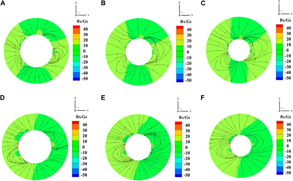
FIGURE 1. The calculated B_x components of the magnetic field for CR2069 at R_ss = 2R_s (A), R_ss = 2.5R_s (B), and R_ss = 3R_s (C), and for CR2217 at R_ss = 2R_s (D), R_ss = 2.5R_s (E) and R_ss = 3R_s (F). The black arrow line represents the magnetic line.

3.2 Calculations of the parameters at different ${\mathit{R}}_{\mathit{s}\mathit{s}}$

There are eight free parameters in the WSA model such as $a_1-a_6$, $V_f$, and $V_s$. These eight parameters will vary with different model initiations, data sources, or the period under study. According to previous studies (Li et al., 2019; Yang et al., 2018), these parameters can be set as $a_1=\frac{2.0}{9.0}$, $a_2=1.0$, $a_3=0.8$, $a_4=0.8$, $a_5=1.05$, $V_s=240.0km/s$, and $V_f=675.0km/s$. The magnetic field structure at $R_{ss}$ as well as $f_s$, ${\theta }_b$, and $V_r$ distributions are then obtained for CR2069 (Figure 2) and CR2217 (Figure 3).

FIGURE 2

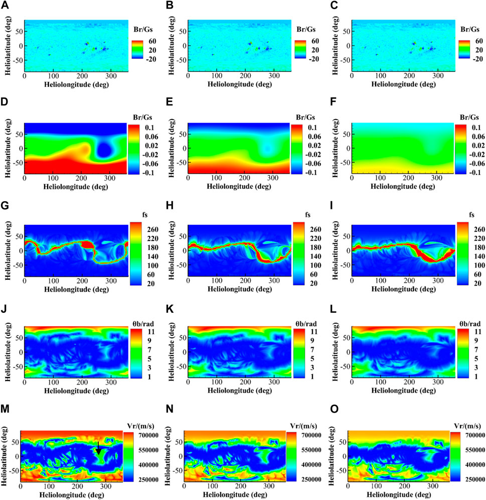
FIGURE 2. The solar wind parameters for CR2069. The abscissa is the longitude of the heliopause and the vertical coordinate is the latitude. The parameters from the first to fifth rows are the magnetic field B_r at 1R_s (A–C), the magnetic field B_r at 1R_ss (D–F), the coronal magnetic field expansion factor f_s (G–I), the minimum angular distance θ_b from the open magnetic line to the coronal hole (J–L), and the solar wind velocity V_r (M–O), respectively. The first column shows the parameters at R_ss = 2R_s (A,D,G,J,M). The second column is the parameters when R_ss = 2.5R_s (B,E,H,K,N). And the third column shows the parameters at R_ss = 3R_s (C,F,I,L,O).

FIGURE 3

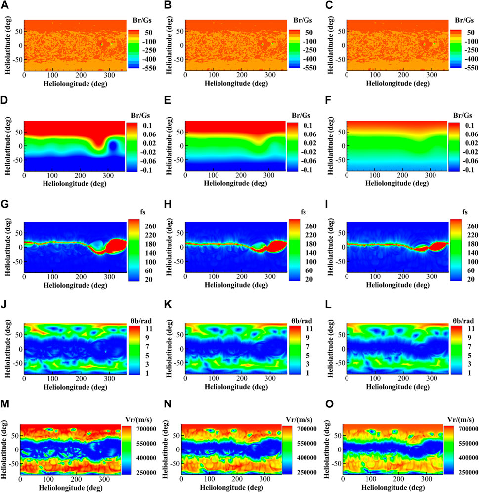
FIGURE 3. The solar wind parameters for CR2217. The abscissa is the longitude of the heliopause and the vertical coordinate is the latitude. The parameters from the first to fifth rows are the magnetic field B_r at 1R_s (A–C), the magnetic field at (D–F), the coronal magnetic field expansion factor (G,–I), the minimum angular distance from the open magnetic line to the coronal hole (J–L), and the solar wind velocity R_ss = 2R_s (M–O), respectively. The first column shows the parameters at (A,D,G,J,M). The second column is the parameters when R_ss = 2.5R_s (B,E,H,K,N). And the third column shows the parameters at R_ss = 3R_s (C,F,I,L,O).

In the fourth row of Figure 2, we can see that the magnetic field in the South Pole region extends north at longitude $0°\sim 230°$, and the magnetic field in the North Pole region extends south at longitude $280°\sim 330°$. This is because in 2008, the extension of polar coronal holes to low latitudes and independent coronal holes of low latitudes were more common (Wang et al., 2009). In the fourth row of Figure 3, the magnetic field in the North Pole region extends southward at longitude $250°\sim 280°$ and in the South Pole region extends northward at longitude $300°\sim 330°$. This is similar to the phenomenon that coronal holes in the polar region extended to low latitudes in 2008. By comparing the polar magnetic field in Figures 2, 3, it can be seen that the magnetic field is evidently reversed. This is due to the solar magnetic polarity cycle changes, resulting in the reversal. In Figures 2, 3, low-latitude regions are covered by low-speed solar wind, while high-latitude regions are covered by high-speed solar wind. This corresponds to the structure of the magnetic line of force corresponding to Figure 1. In Figure 2M, we can see that a low-speed solar wind structure is formed at the longitude of $240°\sim 300°$ and near the latitude of $20°\sim 30°$, which may be related to the pseudo-streamer. Although the foot of the pseudo-streamer is connected with coronal holes of the same polarity, its foot is also close to the boundary of the coronal hole, and the value of the magnetic flow tube θ_b is small, so it can form low-speed solar wind.

Figures 2, 3 yield the following results:

(1) The magnetic field at the source surface will decrease with increasing $R_{ss}$. Through the conservation of magnetic flux (e.g., conservation of the spherical integral of $B_r{r}^2$), increasing $R_{ss}$ will cause the attenuation of magnetic field intensity. Meanwhile, the number of open magnetic field lines that reach the source surface will reduce with increasing $R_{ss}$. The corresponding decrease in the open flux on the source surface further aggravates the decrease in the magnetic field intensity. This conclusion is consistent with that in several previous research studies (Arden et al., 2014; Asvestari et al., 2019; Asvestari et al., 2020; Badman et al., 2020; Lee et al., 2011; Panasenco et al., 2020).

(2) The parameters $f_s$ and ${\theta }_b$ vary slightly as $R_{ss}$ increases, with ${\theta }_b$ decreasing most markedly at high latitudes and $f_s$ at middle and low latitudes. It indicates that the number of magnetic field lines reaching the source surface will decrease as the source surface elevates. In addition, the coronal hole thus shrinks, leading to a decrease in the value of ${\theta }_b$. This conclusion is consistent with that of previous research as well (Arden et al., 2014; Asvestari et al., 2019; Asvestari et al., 2020; Badman et al., 2020; Lee et al., 2011; Panasenco et al., 2020).

(3) The solar wind velocity, $V_r$, decreases with $R_{ss}$, which, in turn, is related to the changes of $f_s$ and ${\theta }_b$.

3.3 Adjusting of WSA model parameters and their effects

According to a previous empirical model (Arge et al., 2003), the solar wind velocity $V_r$ can be calculated as Eq. 3. The $a_1$ reflects the effect of $f_s$ on $V_r$, and $a_2-a_6$ reveal the influence of ${\theta }_b$ on $V_r$. In the WSA model, the optimal values of $a_1-a_6$, $V_f$, and $V_s$ will change over time (Riley et al., 2015).

When the source surface radius $R_{ss}=2.5R_s$ for the CR2069, we set $a_1=2.0/9.0$, $a_2=1.0$, and $a_3=0.8$. Then, we look for the best values of the parameters through adjusting $a_4$, $a_5$,$V_f$, and $V_s$. According to previous studies (Li et al., 2019; Yang et al., 2018), we set $a_4=0.8$, $a_5=1.05$,$V_s=240.0km/s$, and $V_f=675.0km/s$. Afterward, the effect of each parameter on the simulation results is analyzed by adjusting one variable each time, that is, $a_4\pm 0.2$, $a_5\pm 0.2$, $V_f\pm 50.0km/s$, and $V_s\pm 50.0km/s$. Then, the comparison between the observed and simulated $V_r$ at the source surface is shown inFigures 4, 5.

FIGURE 4

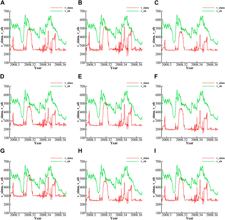
FIGURE 4. Comparison of the observed data and simulated results for different $a_4$, $a_5$, $V_s$, and $V_f$ when $R_{ss}=2.5R_s$. The horizontal coordinate is time (1/365 Day), and the ordinate is solar wind speed (km/s). The red line is the simulated solar wind speed, and the green line is the observed solar wind speed. (A) Comparison obtained from empirical parameter values with $a_4=0.8$, $a_5=1.05$, $V_s=240.0km/s$, and $V_f=675.0km/s$; (B) when $a_4-0.2$; (C) when $a_4+0.2$; (D) when $a_5-0.2$; (E) when $a_5+0.2$; (F) when $V_s-50km/s$; (G) when $V_s+50km/s$; (H) when $V_f-50km/s$; (I) when $V_f+50km/s$.

FIGURE 5

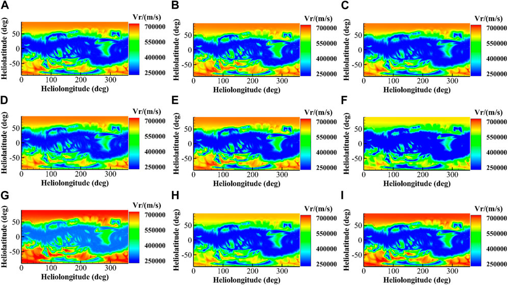
FIGURE 5. Simulated solar wind speed for different $a_4$, $a_5$, $V_s$, and $V_f$ when $R_{ss}=2.5R_s$. (A) The results obtained from empirical parameter values with, $a_4=0.8$, $a_5=1.05$, $V_s=240.0km/s$, and $V_f=675.0km/s$; (B) when $a_4-0.2$; (C) when $a_4+0.2$; (D) when $a_5-0.2$; (E) when $a_5+0.2$; (F) when $V_s-50km/s$; (G) when $V_s+50km/s$; (H) when $V_f-50km/s$; (I) when $V_f+50km/s$.

Figures 4, 5 reveal the following results: (1) a decrease in $a_4$ leads to an overall increase in $V_r$ at middle and low latitudes, and vice versa. However, the change in $a_4$ does not cause significant changes in $V_r$ over high latitudes. (2) A decrease in $a_5$ decreases $V_s$ at middle and low latitudes for faster solar wind and increases it for slower solar winds and vice versa for $a_5$. However, the change in $a_5$ leads to an insignificant change in $V_r$ at high latitudes. (3) An increase in $V_s$ will result in an overall increase in $V_r$, and a decrease in $V_s$ will result in the opposite. (4) The increase in $V_f$ will result in increment of the high-speed flow velocity, while a decrease in $V_f$ does the opposite. However, the variation in $V_f$ has little effect on the low-speed flow.

On the other hand, the variations in MSE, RMSE, and CC are monitored through adjusting different parameters (shown in Table 1). The simulation reveals the results as follows: (1). the decrease in $a_4$ will cause a reduction in MSE and RMSE, and an increase in CC, vice versa. (2). Decreasing $a_5$ will make MSE and RMSE smaller and CC larger, while increasing $a_5$ will do the opposite. (3). An increase in $V_s$ will reduce MSE and RMSE, but CC does not change with $V_s$. (4). Increasing $V_f$ makes MSE and RMSE smaller, but CC does not change. Therefore, for further optimization, we will decrease $a_4$ and $a_5$, and increase $V_s$ and $V_f$ based on the initial setting of $a_4=0.8$, $a_5=1.05$, $V_s=240.0km/s$, and $V_f=675.0km/s$.

TABLE 1

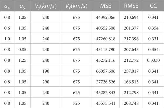
TABLE 1. Values of MSE, RMSE, and CC obtained through parameter tuning with $R_{ss}=2.5R_s$.

3.4 Parameter tuning and quantitative evaluation of the WSA model

In this section, for CR2069 the parameters for the source surface radius $R_{ss}=2.5R_s$ are tuned and refined in order to find the local optimal solutions. The $V_s$ and $V_f$ have a significant impact on the results, which is that $V_s$ determines the extreme value of low–speed solar wind and $V_f$ determines the extreme value of high-speed solar wind. Thus, it can be adjusted through visual comparison (Li et al., 2019). Figure 4A shows that when $a_4=0.8$, $a_5=1.05$, $V_s=240.0km/s$, and $V_f=675.0km/s$, there is a significant difference between the simulated low velocity and the observed low velocity. Therefore, the low-speed flow is adjusted visually to $V_s=330km/s$ to be consistent with the observation data and then $V_f=1000km/s$ to make the high-speed flow match the observation data, as shown in Figure 6.

FIGURE 6

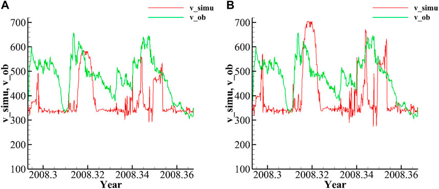
FIGURE 6. (A) Comparison of the observed solar wind speed with the simulated results with the adjustment of $a_4=0.8$, $a_5=1.05$, $V_s=330.0km/s$, and $V_f=675.0km/s$ (A) and then $a_4=0.8$, $a_5=1.05$, $V_s=330.0km/s$, and $V_f=1000.0km/s$ (B), at $R_{ss}=2.5R_s$.

To simplify the calculation, only parameters $a_4$ and $a_5$ will be tuned, with no change after the adjustment of $V_s=330km/s$ and $V_f=1000km/s$. The range of $a_4$ and $a_5$ is from 0 to 1.3 in the step of 0.05, with a total of 729 combinations. Then, the two-dimensional (2D) distribution of RMSE and CC with different $a_4$ and $a_5$ is given in Figure 7, in which we can find a rough parameter space with smaller RMSE and larger CC. In addition, the details of the good results are listed in Table 2. As shown in Figure 7, $a_4=1.2$ and $a_5=0.2$ correspond to RMSE between 80 and 100 with $\mathrm{C}\mathrm{C}=0.42$. When $a_4=0.4$ and $a_5=0.6$, it corresponds to between 100 and 120, with $\mathrm{C}\mathrm{C}=0.38$. For decreasing $a_4$ or $a_5$ individually, the RMSE decreases and CC increases. However, when $a_4$ and $a_5$ change together, the RMSE and CC respond irregularly. Table 2 presents the best results among the 729 simulations, with smaller RMSE and larger CC. Considering the evaluation results, $a_4=0.4$ and $a_5=0.1$ and $a_4=0.25$ and $a_5=0.1$ are selected for the graph, as shown in Figure 8. The RMSE and CC values are significantly optimized through the tuning. From the comparison of Figures 8, 4A, it can be seen that the variation trend of solar wind speed in Figure 8 better agrees with the observation than that in Figure 4. Before and after tuning, RMSE decreased by approximately 135 and CC increased by approximately 0.09. There are two notable structures of solar wind high-speed flow in Figure 8, which originate from low-latitude high-speed flow near longitudes $140°$ and $240°$. This is consistent with the research of Li et al. (2019). Our simulation results can reproduce these high-speed flows with lower peak velocities, but the duration of high-speed flows is consistent with the observed data, and the arrival time of high-speed flows is similar. The maximum velocity of the high-speed flow is evidently underestimated. On one hand, this could be because the tuning parameters have a certain limitation; on the other hand, it may be due to the quality of the observed photospheric magnetic field (Li et al., 2019), and the other limitation is the simplicity of the PFSS model itself.

FIGURE 7

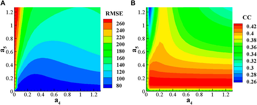
FIGURE 7. When $R_{ss}=2{.5R}_s$, the 2D distribution of RMSE for $a_4$ and $a_5$ (A), and the 2D distribution of CC (B).

TABLE 2

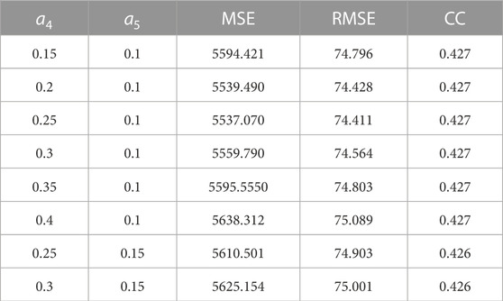
TABLE 2. Values of MSE, RMSE, and CC through tuning of $a_4$ and $a_5$ at $R_{ss}=2.5R_s$.

FIGURE 8

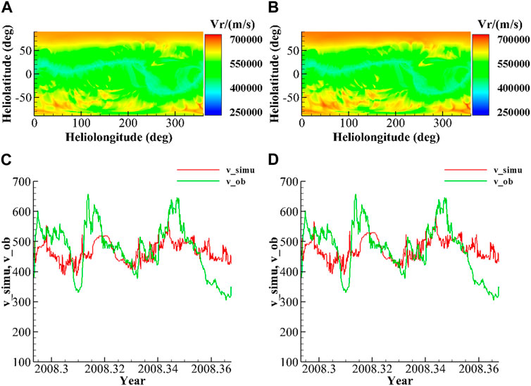
FIGURE 8. Simulated results through parameter tuning with $R_{ss}=2{.5R}_s$. (A) Simulated solar wind speed when $a_4=0.4$, $a_5=0.1$, $V_s=330.0km/s$, and $V_f=1000.0km/s$. (B) The simulated solar wind speed when $a_4=0.25$, $a_5=0.1$, $V_s=330.0km/s$, and $V_f=1000.0km/s$. (C) Comparison of simulated solar wind speed with the observation, with $a_4=0.4$, $a_5=0.1$, $V_s=330.0km/s$, and $V_f=1000.0km/s$. (D) The comparison of simulated solar wind speed with the observation, with $a_4=0.25$, $a_5=0.1$, $V_s=330.0km/s$, and $V_f=1000.0km/s$.

3.5 Effect of ${\mathit{R}}_{\mathit{s}\mathit{s}}$ on the WSA simulation results

From the previous studies, it is clear that the height of the source surface in the coronal magnetic field model affects the values of $f_s$ and ${\theta }_b$ (Arden et al., 2014; Hoeksema et al., 1983; Lee et al., 2011; Sun and Hoeksema. (2009)). Therefore, we set the source surface height as $R_{ss}=2R_s$ and $R_{ss}=3R_s$ to study the specific effects of source surface height variation on physical parameters (Arden et al., 2014; Kruse et al., 2021). The optimization steps are the same as in the $R_{ss}=2{.5R}_s$ case, through tuning $a_4$, $a_5$, $V_s$, and $V_f$. When $R_{ss}=2R_s$, first set $V_s=330km/s$ to make the low-velocity flow consistent with the observed data, and then, we set $V_f=700km/s$ to ensure that the high-speed flow and the observed data match. Based on the fixed $V_s$ and $V_f$, the adjustment range of $a_4$ and $a_5$ is from 0 to 1.3, with the step length of 0.05 and a total combination of 729 simulations. The 2D distribution plots of the RMSE and CC of $a_4$ and $a_5$ (Figures 9A, B) and the distribution table (Table 3) are analyzed. As mentioned in Section 3.4, the decrease in $a_4$ and $a_5$ will give better simulation results. Thus, we select $a_4=0.05$ and $a_5=0.05$ to produce Figure 9C.

FIGURE 9

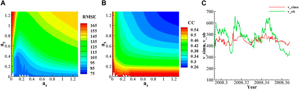
FIGURE 9. (A) When $R_{ss}=2R_s$, the 2D distribution of RMSE for $a_4$ and $a_5$. (B) Two-dimensional distribution of CC for $a_4$ and $a_5$. (C) When $a_4=0.05$ and $a_5=0.05$, the comparison of simulated solar windspeed and observation.

TABLE 3

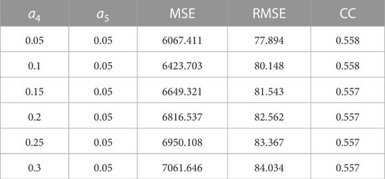
TABLE 3. Values of MSE, RMSE, and CC through tuning of $a_4$ and $a_5$ at $R_{ss}=2R_s$.

When $R_{ss}=3R_s$, we can make a similar adjustment of $V_s=330km/s$ and $V_f=1000km/s$ and then obtain the simulated results given by Figure 10. The 2D distributions of RMSE and CC for $a_4$ and $a_5$ are shown in Figures 10A, B, respectively, and the details of the distribution are exhibited in Table 4. In order to get smaller MSE and RMSE with larger CC, we apply $a_4=0.25$ and $a_5=0.15$ to obtain Figure 10C.

FIGURE 10

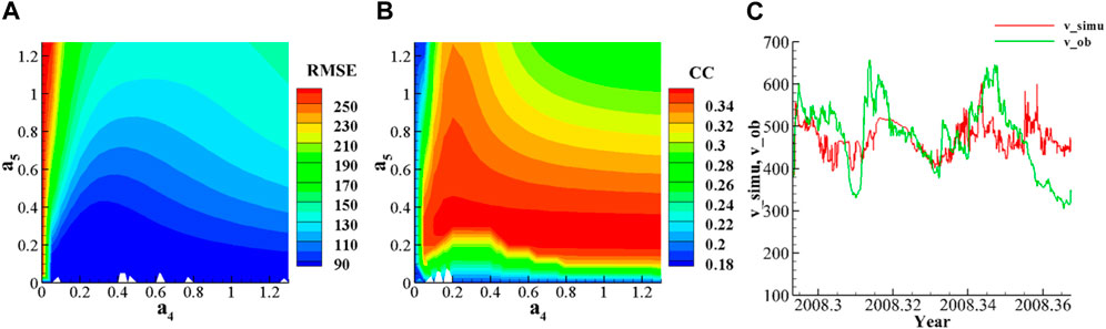
FIGURE 10. (A). When, R_ss= 3R_s, the 2D distribution of RMSE for and a₄ and a₅ (B). The 2D distribution of CC for and a₄ and a₅ (C) When a₄ = 0.25 and a₅ = 0.15, the comparison of simulated solar wind speed and observation.

TABLE 4

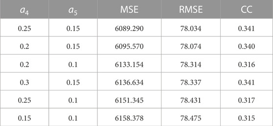
TABLE 4. Values of MSE, RMSE, and CC through tuning of $a_4$ and $a_5$ at $R_{ss}=3R_s$.

It can be seen that the surface heights of the three sources all reproduce the two high-speed flows well, but the peak values and the duration of high-speed flows are not the same. When $R_{ss}=2R_s$, the peak value of the high-speed flow is smaller relative to $R_{ss}=2{.5R}_s$, but the change trend is relatively good. When $R_{ss}=2{.5R}_s$ and $R_{ss}=3R_s$, the peak value of high-speed flow is relatively large, but it is worse than the trend of actual observation data. The reason for underestimating the peak of high-speed flow is the same as in Section 3.4.

Then, the comparison for the MSE, RMSE, and CC at $R_{ss}=2R_s$, $R_{ss}=2{.5R}_s$, and $R_{ss}=3R_s$ shows the following results: (1). when $R_{ss}=3R_s$, the desirable value of RMSE is 78.034. When $R_{ss}=2.5R_s$, the RMSE is relatively small, with a best value of 74.80. When $R_{ss}=2R_s$, the value equals 77.90. Overall, the RMSE exhibits an unremarkable difference at different $R_{ss}$. (2). When $R_{ss}=3R_s$, CC equals 0.34. When $R_{ss}=2.5R_s$, CC is approximately 0.42. When $R_{ss}=2R_s$, CC is approximately 0.55. It is notable that the CC is increasing with decreased $R_{ss}$. Thus, for the PFSS–WSA model, the reduction in $R_{ss}$ can give better simulation results.

Arge and Pizzo. (2000) used the WSA-2000 model to forecast the results for 3 years before and after 1996. The CC between the predicted and observed values is 0.4, and the average relative error is 15%. Owens et al. (2005) used the observed magnetic map of NWO and the PFSS + SCS model to forecast the results from 1995 to 2002. The results show that the RMSE of different years ranges from $75km/s$ to $115km/s$. Gressl et al. (2014) simulated the background solar wind in 2007 using three models: magnetohydrodynamic algorithm outside a sphere/magnetohydrodynamic algorithm outside a sphere (MAS/MAS), MAS/ENLIL, and Wang–Sheeley–Arge/ENLIL (WSA/ENLIL), in which MAS/MAS and MAS/ENLIL significantly overestimated the density of low-velocity flow. Yang et al. (2018) used the MHD model to improve the CC of each parameter. Li et al. (2019) used the MHD model to establish an automated method for systematic quantitative evaluation of simulation results. Compared with these models, the model in this paper adjusts very few parameters and can reproduce the structure of high-speed flow and reflect the variation of source surface height. In addition, when $R_{ss}=2R_s$, the CC can reach 0.42, and the correlation is improved. We believe that the solar source surface should drop appropriately with respect to $R_{ss}=2{.5R}_s$ during the low-solar activity phase of the solar cycle 23. This is consistent with the findings of Lee et al. (2011).

4 Conclusion

In this paper, the PFSS–WSA solar wind model is investigated. This model consists of the PFSS coronal magnetic field extrapolation module and the WSA solar wind velocity module. The PFSS is implemented by the POT3D software package deployed on the Tianhe 1A supercomputer system. In our study, we use the GONG of CR2069 and CR2217 as an inner boundary condition to the PFSS model. It selects the source surface radii $R_{ss}=2R_s$, $R_{ss}=2{.5R}_s$, and $R_{ss}=3R_s$ to initialize the model, in order to obtain the 3D distribution of the coronal magnetic field at different $R_{ss}$. On this basis, the parameters of solar wind velocity $V_r$, coronal magnetic field expansion factor $f_s$, and minimum angular distance of open magnetic field lines from the coronal hole boundary ${\theta }_b$, for the CRs CR2069 and CR2217 are solved within the WSA model.

First, we analyzed the effects of the four free parameters ($a_4$, $a_5$, $V_s$, and $V_f$) in the WSA model on the solar wind velocity. The WSA simulated $V_r$ was compared with the observed data of L1, and we optimized the free parameters by RMSE, MSE, and CC. We found that when $R_{ss}=2{.5R}_s$, we should decrease $a_4$ and $a_5$ and increase $V_s$, and $V_f$ based on $a_4$ = 0.8, $a_5$ = 1.05, $V_s$ = 240.0 km/s, and $V_f$ = 675.0 km/s. After optimization, we finally adjusted the parameters to $a_4$ = 0.4, $a_5$ = 0.1, $V_s$ = 330.0 km/s, and $V_f$ = 1000.0 km/s. After obtaining the solar wind speed at $R_{ss}=2{.5R}_s$, we optimized the free parameters at $R_{ss}=2R_s$ and $R_{ss}=3R_s$. By comparing the evaluation metrics of the three source surface heights, we concluded that the solar source surface should be properly decreased with respect to $R_{ss}=2{.5R}_s$ during the low-solar activity phase of solar cycle 23. This is consistent with the findings of Lee et al. (2011).

However, our current result is highly preliminary. The simple method used to extrapolate the observed solar wind to the corona still needs to account for more complex interaction processes that occur during the propagation of solar wind and the disturbances from CMEs/solar flares through the interplanetary space. Likewise, we need to consider the stream interaction region (SIR), which has some work to take into account (Jian et al., 2015; Li et al., 2019). In addition, we also find that the traditional diagnostic indices, such as RMSE, MSE, and CC, may not reflect the error quality of the forecast comprehensively. Therefore, it is necessary to introduce other error indicators to jointly constrain the tuning process in our simulated results. These are the issues that need further in-depth investigation and improvement in future works.

5 Data access

The photospheric magnetic field data of CR2069 and CR2217 are available from the GONG (https://gong.nso.edu). The observed speed of the solar wind at L1 point comes from the OMNI database run by NASA (http://omniweb.gsfc.nasa.gov). The POT3D software package comes from GitHub (https://github.com/predsci/POT3D).

Data availability statement

The original contributions presented in the study are included in the article/Supplementary Material; further inquiries can be directed to the corresponding author.

Author contributions

XZ performed data analysis and wrote the manuscript. SQ conceived this study and wrote the manuscript. WS was in charge of the organization and English editing of the whole manuscript. HY made some contributions on the discussions of the manuscript. All authors contributed to the article and approved the submitted version.

Funding

This work is supported by the National Natural Science Foundation of China (No. 41974178).

Acknowledgments

The authors acknowledge the use of a supercomputer system provided by the Tianhe 1A Center, Tianjin, China. The authors thank Dr. Huichao Li of Harbin Institute of Technology, Shenzhen, for his help on discussions.

Conflict of interest

The authors declare that the research was conducted in the absence of any commercial or financial relationships that could be construed as a potential conflict of interest.

Publisher’s note

All claims expressed in this article are solely those of the authors and do not necessarily represent those of their affiliated organizations, or those of the publisher, the editors, and the reviewers. Any product that may be evaluated in this article, or claim that may be made by its manufacturer, is not guaranteed or endorsed by the publisher.

References

Allen, D. M. (1971). Mean square error of prediction as a criterion for selecting variables. Technometrics 13, 469–475. doi:10.1080/00401706.1971.10488811

CrossRef Full Text | Google Scholar

Altschuler, M. D., Levine, R. H., Stix, M., and Harvey, J. (1977). High resolution mapping of the magnetic field of the solar corona. Sol. Phys. 51 (2), 345–375. doi:10.1007/bf00216372

CrossRef Full Text | Google Scholar

Altschuler, M. D., and Newkirk, G. (1969). Magnetic fields and the structure of the solar corona. Sol. Phys. 9 (1), 131–149. doi:10.1007/bf00145734

CrossRef Full Text | Google Scholar

Arden, W. M., Norton, A. A., and Sun, X. (2014). A “breathing” source surface for cycles 23 and 24. J. Geophys. Res. Space Phys. 119 (3), 1476–1485. doi:10.1002/2013ja019464

CrossRef Full Text | Google Scholar

Arge, C. N., Odstrcil, D., Pizzo, V. J., and Mayer, L. R. (2003). Improved method for specifying solar wind speed near the Sun. AIP Conf. Proc. 679 (1), 190–193. doi:10.1063/1.1618574

CrossRef Full Text | Google Scholar

Arge, C. N., and Pizzo, V. J. (2000). Improvement in the prediction of solar wind conditions using near-real time solar magnetic field updates. J. Geophys. Res. Space Phys. 105 (5), 10465–10479. doi:10.1029/1999ja000262

CrossRef Full Text | Google Scholar

Asuero, A. G., Sayago, A., and González, A. (2006). The correlation coefficient: an overview. Crit. Rev. Anal. Chem. 36 (1), 41–59. doi:10.1080/1040834050052-6766

CrossRef Full Text | Google Scholar

Asvestari, E., Heinemann, S. G., Temmer, M., Pomoell, J., Kilpua, E., Magdalenic, J., et al. (2019). Reconstructing coronal hole areas with EUHFORIA and adapted WSA model: optimizing the model parameters. J. Geophys. Res. Space Phys. 124 (11), 8280–8297. doi:10.1029/2019ja027173

CrossRef Full Text | Google Scholar

Asvestari, E., Heinemann, S. G., Temmer, M., Pomoell, J., Kilpua, E., Magdalenic, J., et al. (2020). The impact of coronal hole characteristics and solar cycle activity in reconstructing coronal holes with EUHFORIA. J. Phys. Conf. Ser. 1548 (1), 012004. doi:10.1088/1742-6596/1548/1/012004

CrossRef Full Text | Google Scholar

Badman, S. T., Bale, S. D., Martínez Oliveros, J. C., Panasenco, O., Velli, M., Stansby, D., et al. (2020). Magnetic Connectivity of the Ecliptic Plane within 0.5 au: potential Field Source Surface Modeling of the First Parker Solar Probe Encounter. Astrophysical J. Suppl. Ser. 246 (2), 23. doi:10.3847/1538-4365/ab4da7

CrossRef Full Text | Google Scholar

Baker, D. N. (2002). How to cope with space weather. Science 297 (5586), 1486–1487. doi:10.1126/science.1074956

PubMed Abstract | CrossRef Full Text | Google Scholar

Cao, E. (2012). Solar storms and their impact on human social activities. Spacecr. Environ. Eng. 29 (3), 237. doi:10.3969/j.issn.1673-1379.2012.03.001

CrossRef Full Text | Google Scholar

Caplan, R., Downs, C., Linker, J., and Mikic, Z. (2021). Variations in finite–difference potential fields. Astrophysical J. 915, 44. doi:10.3847/1538-4357/abfd2f

CrossRef Full Text | Google Scholar

Caplan, R. M., Downs, C., and Linker, J. A. (2016). Synchronic coronal hole mapping using multi-instrument EUV images: data preparation and detection method. Astrophysical J. 823, 53. doi:10.3847/0004-637x/823/1/53

CrossRef Full Text | Google Scholar

Chai, T., and Draxler, R. R. (2014). Root mean square error (RMSE) or mean absolute error (MAE). Geosci. Model. Dev. Discuss. 7 (1), 1525–1534. doi:10.5194/gmd-7-1247-2014

CrossRef Full Text | Google Scholar

Eastwood, J. P., Biffis, E., Hapgood, M. A., Green, L., Bisi, M. M., Bentley, R. D., et al. (2017). The economic impact of space weather: where do we stand? Risk Anal. 37 (2), 206–218. doi:10.1111/risa.12765

PubMed Abstract | CrossRef Full Text | Google Scholar

Feng, X., Li, C., Xiang, C., Zhang, M., Li, H., and Wei, F. (2017). Data-driven modeling of the solar corona by a new three-dimensional path-conservative osher–solomon MHD model. Astrophysical J. Suppl. Ser. 233 (1), 10. doi:10.3847/1538-4365/aa957a

CrossRef Full Text | Google Scholar

Feng, X., Liu, X., Xiang, C., Li, H., and Wei, F. (2019). A new MHD model with a rotated-hybrid scheme and solenoidality-preserving approach. Astrophysical J. 871 (2), 226. doi:10.3847/1538-4357/aafacf

CrossRef Full Text | Google Scholar

Feng, X. S., Xiang, C. Q., and Zhong, D. K. (2013). Numerical study of interplanetary solar storms (in Chinese). Sci. Sin. Terrae 43, 912–933. doi:10.1360/zd-2013-43-6-912

CrossRef Full Text | Google Scholar

Feng, X. S., Xiang, C. Q., and Zhong, D. K. (2011). The state–of–art of three–dimensional numerical study for corona–interplanetary process of solar storms (in Chinese). Sci. Sin–Terrae 41, 1–28. doi:10.3724/SP.J.1011.2011.00181

CrossRef Full Text | Google Scholar

Gressl, C., Veronig, A. M., Temmer, M., Odstrčil, D., Linker, J. A., Mikić, Z., et al. (2014). Comparative study of MHD modeling of the background solar wind. Sol. Phys. 289 (5), 1783–1801. doi:10.1007/s11207-013-0421-6

CrossRef Full Text | Google Scholar

Hoeksema, J. T., and Scherrer, P. H. (1986). An atlas of photospheric magnetic field observations and computed coronal magnetic fields: 1976–1985. Sol. Phys. 105 (1), 205–211. doi:10.1007/bf00156388

CrossRef Full Text | Google Scholar

Hoeksema, J. T., Wilcox, J. M., and Scherrer, P. H. (1982). Structure of the heliospheric current sheet in the early portion of Sunspot Cycle 21. J. Geophys. Res. Space Phys. 87 (12), 10331–10338. doi:10.1029/ja087ia12p10331

CrossRef Full Text | Google Scholar

Hoeksema, J. T., Wilcox, J. M., and Scherrer, P. H. (1983). The structure of the heliospheric current sheet: 1978–1982. J. Geophys. Res. Space Phys. 88 (A12), 9910–9918. doi:10.1029/ja088ia12p09910

CrossRef Full Text | Google Scholar

Jian, L. K., MacNeice, P. J., Taktakishvili, A., Odstrcil, D., Jackson, B., Yu, H. S., et al. (2015). Validation for solar wind prediction at Earth: comparison of coronal and heliospheric models installed at the CCMC. Space weather. 13 (5), 316–338. doi:10.1002/2015sw001174

CrossRef Full Text | Google Scholar

Kruse, M., Heidrich-Meisner, V., and Wimmer-Schweingruber, R. F. (2021). Evaluation of a potential field source surface model with elliptical source surfaces via ballistic back mapping of in situ spacecraft data. Astronomy Astrophysics 645 (1), A83. doi:10.1051/0004-6361/202039120

CrossRef Full Text | Google Scholar

Kruse, M., Heidrich-Meisner, V., Wimmer-Schweingruber, R., and Hauptmann, M. (2020), An elliptic expansion of the potential field source surface model.

CrossRef Full Text | Google Scholar

Lee, C. O., Luhmann, J. G., Hoeksema, J. T., Sun, X., Arge, C. N., and de Pater, I. (2011). Coronal field opens at lower height during the solar cycles 22 and 23 minimum periods; IMF comparison suggests the source surface should Be lowered. Sol. Phys. 269 (2), 367–388. doi:10.1007/s11207-010-9699-9

CrossRef Full Text | Google Scholar

Levine, R. H., Schulz, M., and Frazier, E. N. (1982). Simulation of the magnetic structure of the inner heliosphere by means of a non-spherical source surface. Sol. Phys. 77 (1), 363–392. doi:10.1007/bf00156118

CrossRef Full Text | Google Scholar

Li, H. C., Feng, X. S., and Xiang, C. Q. (2019). Time–dependments simulation and result validation of interplanetary solar wind. Chin. J. Geophys. 62 (1), 1–18. doi:10.6038/cjg2019L0625

CrossRef Full Text | Google Scholar

Mackay, D. H., and Yeates, A. R. (2012). The sun’s global photospheric and coronal magnetic fields: observations and models. Living Rev. Sol. Phys. 9 (1), 6. doi:10.12942/lrsp-2012-6

CrossRef Full Text | Google Scholar

Mikić, Z., Downs, C., Linker, J. A., Caplan, R. M., Mackay, D. H., Upton, L. A., et al. (2018). Predicting the corona for the 21 August 2017 total solar eclipse. Nat. Astron. 2 (11), 913–921. doi:10.1038/s41550-018-0562-5

CrossRef Full Text | Google Scholar

Nikolj, L., and Trichtchenko, L. (2012). Development of coronal field and solar wind components for MHD interplanetary simulations, world Academy of science, engineering and technology. Int. J. Environ. Chem. Ecol. Geol. Geophys. Eng. 6, 698–702. doi:10.5281/zenodo.1062642

CrossRef Full Text | Google Scholar

Owens, M. J., Arge, C. N., Spence, H. E., and Pembroke, A. (2005). An event-based approach to validating solar wind speed predictions: high-speed enhancements in the Wang-Sheeley-Arge model. J. Geophys. Res. Space Phys. 110 (12), A12105. doi:10.1029/2005ja011343

CrossRef Full Text | Google Scholar

Panasenco, O., Velli, M., D’Amicis, R., Shi, C., Réville, V., Bale, S. D., et al. (2020). Exploring Solar Wind Origins and Connecting Plasma Flows from the Parker Solar Probe to 1 au: nonspherical Source Surface and Alfvénic Fluctuations. Astrophysical J. Suppl. Ser. 246 (2), 54. doi:10.3847/1538-4365/ab61f4

CrossRef Full Text | Google Scholar

Parker, E. N. (1958). Dynamics of the interplanetary gas and magnetic fields. Astrophysical J. 128, 664. doi:10.1086/146579

CrossRef Full Text | Google Scholar

Riley, P., Baker, D., Liu, Y. D., Verronen, P., Singer, H., and Güdel, M. (2018). Extreme space weather events: from cradle to grave. Space Sci. Rev. 214 (1), 21–24. doi:10.1007/s11214-017-0456-3

CrossRef Full Text | Google Scholar

Riley, P., Linker, J. A., and Arge, C. N. (2015). On the role played by magnetic expansion factor in the prediction of solar wind speed. Space weather. 13, 154–169. doi:10.1002/2014sw001144

CrossRef Full Text | Google Scholar

Riley, P., Linker, J. A., Mikić, Z., Lionello, R., Ledvina, S. A., and Luhmann, J. G. (2006). A comparison between global solar magnetohydrodynamic and potential field source surface model results. Astrophysical J. 653 (2), 1510–1516. doi:10.1086/508565

CrossRef Full Text | Google Scholar

Robinson, R. M., and Behnke, R. A. (2001). The U.S. National space weather program: a retrospective. Geophys. Monogr. Ser. 2001, 1–10. doi:10.1029/GM125p0001

CrossRef Full Text | Google Scholar

Sahade, A., Cécere, M., and Krause, G. (2020). Influence of coronal holes on CME deflections: numerical study. Astrophysical J. 896 (1), 53. doi:10.3847/1538-4357/ab8f25

CrossRef Full Text | Google Scholar

Schatten, K. (1971). Current sheet model for the solar corona. Cosm. Electrodyn. 2, 2.

Google Scholar

Schatten, K. H., Wilcox, J. M., and Ness, N. F. (1969). A model of interplanetary and coronal magnetic fields. Sol. Phys. 6 (3), 442–455. doi:10.1007/bf00146478

CrossRef Full Text | Google Scholar

Schulz, M., Frazier, E. N., and Boucher, D. J. (1978). Coronal magnetic-field model with non-spherical source surface. Sol. Phys. 60 (1), 83–104. doi:10.1007/bf00152334

CrossRef Full Text | Google Scholar

Schulz, M. (1997). Non-spherical source-surface model of the heliosphere: a scalar formulation. Ann. Geophys. 15 (11), 1379–1387. doi:10.1007/s00585-997-1379-1

CrossRef Full Text | Google Scholar

Schwenn, R. (2006). Space weather: the solar perspective. Living Rev. Sol. Phys. 3 (1), 2. doi:10.12942/lrsp-2006-2

CrossRef Full Text | Google Scholar

Sun, X., and Hoeksema, J. T. (2009). A new source surface radius in potential field modeling during the current weak solar minimum? arXiv.

Google Scholar

Thompson, W. (2006). Coordinate systems for solar image data. Astronomy Astrophysics 449, 791–803. doi:10.1051/0004-6361:20054262

CrossRef Full Text | Google Scholar

Tóth, G., van der Holst, B., and Huang, Z. (2011). Obtaining potential field solutions with spherical harmonics and finite differences. Astrophysical J. 732 (2), 102. doi:10.1088/0004-637x/732/2/102

CrossRef Full Text | Google Scholar

Wang, Y. L., and Yuan, L. (2021). Tianhe bright interviewed meng xiangfei, assistant director of national supercomputing Tianjin center. Talents 01, 32–35.

Google Scholar

Wang, Y. M., Robbrecht, E., and Sheeley, N. R. (2009). ON the weakening of the polar magnetic fields during solar cycle 23. Astrophysical J. 707 (2), 1372–1386. doi:10.1088/0004-637x/707/2/1372

CrossRef Full Text | Google Scholar

Wang, Y. M., and Sheeley, N. R. (1990). Solar wind speed and coronal flux–tube expansion. Astrophysical J. 355, 726. doi:10.1086/168805

CrossRef Full Text | Google Scholar

Yang, Z. C., Shen, F., and Yang, Y. (2018). Three–dimensional MHD simulation of interplantary solar wind. Chin. J. Geophys 61 (11), 4337–4347. doi:10.6038/cjg2018L0515

CrossRef Full Text | Google Scholar