Equatorial plasma bubbles features over the Brazilian sector according to the solar cycle and geomagnetic activity level

Equatorial plasma bubbles (EPBs) can lead to signal degradation, affecting the measurement accuracy. Studying EPBs and their characteristics has gained increasing importance. The characteristics of EPBs were investigated using the rate of total electron content (TEC) index (ROTI) maps under different solar and magnetic activity conditions during two periods: July 2014–July 2015 (solar maximum activity with F10.7: 145.9 × 10⁻²² W⋅m⁻²⋅Hz⁻¹) and July 2019–July 2020 (solar minimum activity with F10.7: 69.7 × 10⁻²² W⋅m⁻²⋅Hz⁻¹). We also divided this analysis according to the magnetic activity levels based on Kp and Dst (disturbance storm time) indices, classified as follows: quiet+ (Kp ≤3 and Dst >−30 nT), quiet− (Kp ≤3 and Dst <−30 nT), disturbed weak (−50 nT <Dst ≤−30 nT), moderate (−100 nT <Dst ≤−50 nT), and intense (Dst ≤−100 nT). The ROTI is calculated using the slant TEC with the carrier phase, and its keograms are used to extract the zonal velocity and distance. Our statistical investigation shows the occurrence rate, duration, zonal drift velocity, and inter-bubble zonal distance of EPBs over the Brazilian sector. The latitudinal extension and zonal drift velocity of EPBs are higher during the solar maximum than those in the solar minimum. In addition, EPBs are found with unusually long durations, remaining until the morning (∼12 UT), and 10% of EPB observations occurred on the winter solstice.

Highlights

• ROTI maps were used to study the characteristics of EPBs over the Brazilian sector for different solar and magnetic activities.

• The magnetic activity was divided according to Kp and Dst indices.

• There are significant differences in the behavior of EPBs between quiet and disturbed periods and between the solar maximum and minimum.

1 Introduction

Equatorial plasma bubbles (EPBs) have been extensively studied globally (e.g., Burke et al., 2004; Nishioka et al., 2008; Kepkar et al., 2020), especially over the Brazilian sector (e.g., Abdu et al., 2003; Pimenta et al., 2003; Abdu et al., 2009; Paulino et al., 2011; Abdu et al., 2012; Takahashi et al., 2014; Takahashi et al., 2015). EPBs are well-known as large-scale ionospheric plasma depletions that occur at the magnetic equator, elongating along the magnetic field lines (Rishbeth, 2000). The Rayleigh–Taylor instability (RTI) is the main mechanism that initiates EPBs (Haerendel, 1973; Kelley, 2009), with driving from the rapid uplift of equatorial F-layer (E × B) perturbations on its bottom side. These irregularities can cause signal degradation in global navigation satellite systems (GNSS), such as cycle slips and a loss of lock, which significantly impact the measurement accuracy. Consequently, the study of EPBs and their characteristics has become increasingly important (Ansari et al., 2023).

Studies have focused on investigating the EPB characteristics (e.g., occurrence rate, duration, zonal drift velocity, inter-bubble zonal distance, and latitudinal extension) and how they vary monthly, seasonally, and with solar and magnetic activities (e.g., Nishioka et al., 2008; Kumar, 2017; Li et al., 2020; Timoçin et al., 2020). Nishioka et al. (2008) performed an EPB occurrence study using global positioning system (GPS) receiver data collected from 2000 to 2006. The authors showed that December solstice occurrences were higher than those at the June solstice over the Atlantic sector. On the other hand, Li et al. (2020) studied the EPB occurrence rate in Hong Kong between 2013 and 2019, and they showed that the most significant occurrence was on the equinoxes. Similar findings were reported by Kumar (2017) in the Indian sector and Sun et al. (2016) in the Chinese sector. These authors revealed a high occurrence of EPBs on equinoxes during both solar maximum and minimum periods.

The occurrence patterns of EPBs over the Brazilian sector showed distinct characteristics compared to other regions of the globe. In general, EPBs in Brazilian stations are observed during nighttime hours in the summer months and last 4–6 h (Sobral et al., 2002). Barros et al. (2018) analyzed total electron content (TEC) maps over the Brazilian sector for the period from 2012 to 2016, showing that the months between September and March had the highest number of EPB occurrences. Furthermore, the authors showed the presence of a latitudinal gradient in both the zonal drift velocity and inter-bubble zonal distance of EPBs, consistent with previous studies (Sobral et al., 1981; Pimenta et al., 2003; Barros et al., 2018). The zonal drift velocity varies from ∼200 m/s at the equator to ∼50 m/s at low latitudes. In comparison, the inter-bubble zonal distance ranges from ∼1,000 to 600 km, from the equator to 30° latitude. In addition, EPBs can exhibit a latitudinal extension of ±35° (Barros et al., 2018).

Another focus is the geomagnetic storm effects on EPB generation and evolution (e.g., Aarons, 1991; Fejer et al., 1991; Sastri et al., 2002; Abdu et al., 2003; Huang et al., 2005; Tulasi Ram et al., 2008; Wan et al., 2019; Timoçin et al., 2020; Vankadara et al., 2022). Timoçin et al. (2020) observed the suppression of EPBs during the St. Patrick’s Day 2015 geomagnetic storm in the Indian sector. The authors attributed that this behavior could be caused by westward disturbance dynamo electric fields (DDEFs) or eastward prompt penetration electric fields (PPEFs). They concluded that the electric field induces a downward movement of the equatorial F-region at dusk, inhibiting the RTI. A recent study by Ogwala et al. (2022) about the ionospheric irregularity characteristics over Nigeria shows that the enhancement or suppression of ionospheric irregularities during a geomagnetic storm is influenced by the local time of the sudden storm commencement (SSC), determining when electric fields penetrate equatorial/low latitudes. Furthermore, Abdu et al. (2009) observed two different effects of geomagnetic storms on EPBs in the Brazilian sector, which are as follows: 1) EPB suppression due to the westward PPEF and 2) EPB intensification when the polarity of the electric field is eastward, improving the pre-reversal enhancement (PRE) conditions. During geomagnetic storms, EPBs can exhibit atypical behavior, with latitudinal extensions exceeding 40° compared to the geomagnetically quiet periods (e.g., Huang et al., 2007; Cherniak and Zakharenkova, 2016; Li et al., 2018). These expanded latitudinal extensions imply that the apex height of EPBs can vary from ∼300 to ∼2,500 km (Ma et al., 2020). In addition, Vankadara et al. (2022) studied the evolution and drifting features of plasma irregularities over India during geomagnetic storms. Their findings revealed the presence of plasma irregularities at the equator, which subsequently expanded poleward with a time delay.

The main purpose of this work is to study the occurrence and characteristics of EPBs, and to compare their variability according to the solar activity and geomagnetic disturbance levels. Since most statistical studies analyzed EPBs without implying the geomagnetic disturbance levels, our analysis contributes to enhancing the understanding of EPB characteristics in the context of geomagnetic disturbances and solar activity. The analyzed period was from July 2014 to July 2015 (solar maximum) and July 2019 to July 2020 (solar minimum). The rate of TEC index (ROTI) map is used as a methodology for detecting EPB structures, and keograms are used to obtain the zonal velocity and distance. Our findings indicate that the latitudinal extension and zonal drift velocity of EPBs were reduced during the solar minimum compared to the solar maximum. Furthermore, this study presents observations of EPBs exhibiting an atypical behavior during geomagnetically disturbed periods, including prolonged durations with EPBs persisting into the morning hours (∼12 UT), occurrences of pre-dawn EPBs, and approximately 10% of EPBs observed on the winter solstice. Therefore, this paper is organized as follows: Section 2 presents the methodology used in this work, divided into 1) the dataset and 2) the ROTI calculation. The results and discussions are presented in Section 3, which is separated into three topics related to EPB characteristics. Finally, in Section 4, we summarize the conclusions of this work.

2 Methodology

2.1 The dataset

The Brazilian network for continuous monitoring of the GNSS systems (RBMC), as shown in Figure 1, was used to estimate the ROTI over the Brazilian sector. Furthermore, the Kp and Dst indices are both measures used to quantify the level of magnetic activity or disturbances in the Earth’s magnetosphere. The Kp index is a global geomagnetic activity index that provides a measure of the average disturbance level of the Earth’s magnetic field over a specific time interval. It ranges from 0 to 9, where values from 0 to 3 indicate quiet periods, while values from 4 to 9 represent disturbed periods (e.g., Fejer et al., 1991; Liu et al., 2018). On the other hand, the Dst index is a measure of the strength and intensity of geomagnetic storms that occur in the Earth’s equatorial region. It is commonly used to distinguish different levels of geomagnetic storm activity (e.g., Gonzalez et al., 1994).

FIGURE 1

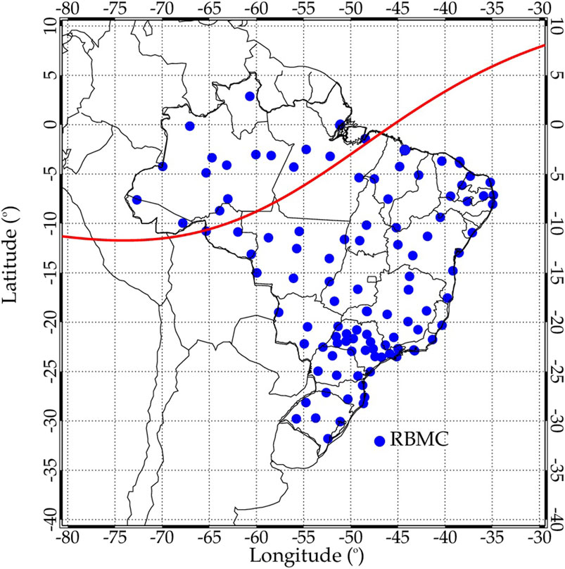
FIGURE 1. Location of the Brazilian network for the continuous monitoring of the GNSS (RBMC). The red line is the magnetic equator for the year 2015 at a 350-km altitude.

The datasets were further subdivided according to the level of magnetic activity into quiet (Kp ≤3) and disturbed (Kp >3) periods, considering their hourly average. The quiet period was subdivided into quiet+ (Kp ≤3 and Dst >−30 nT) and quiet− (Kp ≤3 and Dst <−30 nT) periods. The disturbed period was categorized into 1) weak (−50 nT <Dst ≤−30 nT), 2) moderate (−100 nT <Dst ≤−50 nT), and 3) intense (Dst ≤−100 nT), according to Gonzalez et al. (1994). All categories are summarized in Table 1.

TABLE 1

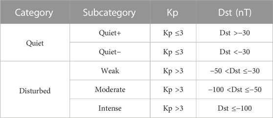
TABLE 1. The quiet category is subcategorized into quiet+ and quiet− periods, and the disturbed category is subcategorized into weak, moderate, and intense periods, where they are established according to Kp and Dst indices.

Furthermore, the characteristics of EPBs are presented as a function of the solar cycle. The data collected between July 2014 and July 2015 (F10.7: 145.9 × 10⁻²² W⋅m⁻²⋅Hz⁻¹) represent the solar maximum activity, while the period between July 2019 and July 2020 (F10.7: 69.7 × 10⁻²² W⋅m⁻²⋅Hz⁻¹) represents the solar minimum activity.

2.2 The ROTI calculation

In this work, we use ROTI maps to detect EPBs. We used the slant TEC (STEC) to obtain the ROTI calculated using the carrier phase (Eq. 1). Carrier phases are obtained from the receiver-independent exchange format (RINEX) file for each satellite–GNSS receiver pair, with a 15-s sampling interval.

$STEC=\left(\frac{L_1}{f_1}-\frac{L_2}{f_2}\right)\frac{f_1^2{f}_2^2}{f_1^2-f_2^2}\frac{c}{K},(1)$

where the frequencies $f_1$ and $f_2$ are 1575.42 and 1227.60 MHz, respectively. $L_1$ and $L_2$ are the phase measurements corresponding to $f_1$ and $f_2$, K is 40.3 m³/s², and c is the speed of light. Only elevation angles greater than 30° were computed.

After that, the rate of TEC (ROT) is found by the STEC difference between two measurements ($∆STEC$) divided by the time difference in the same interval ($∆\mathrm{t}$).

$ROT=\frac{∆STEC}{∆\mathrm{t}}.(2)$

This calculation is performed for each pseudorandom noise (PRN) separately. Following this, we performed a detrended ROT for 30 s.

The standard deviation of the detrended ROT is the ROTI, given by Eq. 3 (Pi et al., 1997). The ROTI time resolution is 5 min.

$ROTI=\sqrt{<detrended\left(ROT\right)²>-<detrended\left(ROT\right){>}^2}.(3)$

The ROTI has a scale length of approximately 6 km, which is widely accepted for EPB detection as in most cases, a single EPB can extend up to 5° (∼600 km) in longitude and 20° (∼2,200 km) in latitude (Barros et al., 2018). ROTI maps are generated every 10 min. Figure 2 shows the ROTI map at the ionospheric piercing point (IPP) height of 350 km for each PRN (Figure 2A) and interpolated to cover the entire Brazilian sector (Figure 2B). Interpolation is performed for 1 × 1 element, corresponding to 0.5° × 0.5° observation cells in the latitude and longitude. If no data cover this area, the cell is resized for 3 × 3 elements, corresponding to 1.5° × 1.5°. This method is applied in up to 21 × 21 elements corresponding to 10.5° × 10.5° (Takahashi et al., 2016).

FIGURE 2

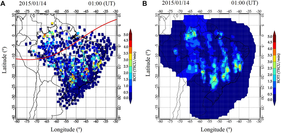
FIGURE 2. (A) ROTI map on the IPP, at 01:00 UT on 14 January 2015, and (B) same ROTI map using the interpolation method.

The characteristics of EPBs were studied using the ROTI keogram methodology, as described in previous studies (e.g., Buhari et al., 2015; Buhari et al., 2017). The ROTI keogram is a ROTI data collection displayed as a geographic longitude vs. the universal time (UT) diagram, as shown in Figure 3A. The method to obtain the keograms is based on the fixed geographic latitudes in ROTI maps. The fixed geographic latitudes considered were 0°S, 5°S, 10°S, 15°S, 20°S, 25°S, 30°S, and 35°S, as shown in Figure 3B.

FIGURE 3

FIGURE 3. (A) Sequence of ROTI maps from 21 to 08 UT on 13 and 14 January 2014, and (B) ROTI keograms for fixed geographic latitudes of 0°S, 5°S, 10°S, 15°S, 20°S, 25°S, 30°S, and 35°S.

Figure 3A shows a sequence of ROTI maps, while Figure 3B shows elongated structures propagating eastward, which are identified as meridionally oriented EPBs at each fixed latitude. Thus, with the detection of these structures, it becomes feasible to calculate the zonal distance between two structures ($d_E$) and the zonal drift velocity ($v_E)$, given by the line passing through the middle of each structure, according to Eqs 4, 5:

$d_E={Lon}_2-{Lon}_1(4)$

and

$v_E=\frac{{Lon}_{{\mathrm{t}}_2}-{Lon}_{{\mathrm{t}}_1}}{{\mathrm{t}}_2-{\mathrm{t}}_1},(5)$

where Lon is the longitude and t is the time.

The zonal distance and zonal drift velocity calculation methodology were validated in previous works using TEC and ROTI keograms (e.g., Buhari et al., 2014; Barros et al., 2018).

Finally, some procedures were established to consider the structures observed as EPBs:

a) The ROTI must present values greater than 1 TECU/min (e.g., Zakharenkova and Cherniak, 2021).

b) The duration must be longer than 1 h (e.g., Barros et al., 2018).

c) The detected structure must be well-defined, with elongations greater than 10° latitude (e.g., Barros et al., 2018).

3 Results and discussions

3.1 Characteristics of EPBs observed in the quiet period

In this analysis, a total of 231 days were identified as the quiet period (Kp ≤3) at the solar maximum, with 106 days (45.9%) exhibiting EPB occurrences. During the solar minimum, 330 quiet days were observed, with 156 EPB detections (47.3%). Figure 4 shows the occurrence rate for (a) the solar maximum activity (red scale) and (b) the solar minimum activity (blue scale) in this period. The y-axis shows the month of observation, and the x-axis refers to UT. The black dotted vertical lines are the dusk and dawn terminators at an altitude of 350 km (the same as the IPP height).

FIGURE 4

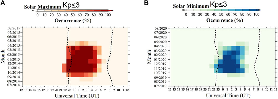
FIGURE 4. EPB occurrence for the period of (A) solar maximum in red (from July 2014 to July 2015) and (B) solar minimum in blue (from July 2019 to July 2020) during a quiet period (Kp ≤3). The black dotted vertical lines are the dusk and dawn terminators at a 350-km altitude.

It should be noted that in Figure 4, EPB occurrences were more frequent during the solar maximum than those in the solar minimum, as expected from the findings of previous studies (Basu et al., 2002; Xiong et al., 2010; Kumar, 2017). The peak occurrences were between October and March, from 22 UT to 5 UT (Sobral et al., 2002; Barros et al., 2018), in both solar activities. The seasonal pattern also shows a good agreement with the seasonal variation found in the literature (Burke et al., 2004; Barros et al., 2018; Kepkar et al., 2020). The observed seasonality has been attributed to the seasonal variation of the PRE, which controls EPB generation and development (Abdu et al., 1981; Tsunoda, 1985; Sobral et al., 2002). This enhancement happens when thermosphere winds interact with the ionospheric conductivity along the sunset terminator. The geomagnetic field declinations can affect the PRE and EPB seeding. Specifically, the geomagnetic field declination over the Brazilian region is higher (∼20°W) than that in other locations, creating different seasonal conditions (Abdu et al., 1981; Sobral et al., 2002). Tsunoda (1985) demonstrated that the geomagnetic declination influences the seasonal patterns of irregularity occurrence globally, using data from radio-wave scintillation. The authors found that the influence of the geomagnetic declination and geographic latitude of the dip equator governs the seasonal variation. They observed that the highest scintillation occurrences are on the December solstice as the negative (westward) declination increases in the American–African region. Similarly, the highest scintillation occurrences are observed in the June solstice in the Indian–Pacific region, which appears to be connected to a corresponding gradual rise in the positive (eastward) declination.

To discuss the differences between solar activity, we divided the analysis into quiet+ (Kp ≤3 and Dst >−30 nT) and quiet− (Kp ≤3 and Dst <−30 nT) periods, as mentioned previously. Figure 5 shows a histogram of the number of EPB occurrences for quiet+ (left side) and quiet− (right side) periods by fixed geographic latitudes (0°S, 5°S, 10°S, 15°S, 20°S, 25°S, 30°S, and 35°S) (Figure 5A). Figure 5B shows the mean values of the zonal drift velocity ($v_E$) for the eight fixed latitudes, and Figure 5C refers to the number of measurements available for distance calculations. It is important to mention that each distance measurement requires at least two structures. Lastly, Figure 5D shows the mean value of the zonal distance between two structures ($d_E$) for the fixed latitudes. Error bar sizes in Figure 5 represent the standard deviation. The red bars represent the analysis during the solar maximum, and the blue bars refer to the solar minimum. The black lines represent a linear fitting, from which a zonal drift latitudinal gradient ($\nabla v_E$) and a zonal distance gradient ($\nabla d_E$) were calculated (Barros et al., 2018). Additionally, in this figure, we present the regression equations that demonstrate the zonal distance gradient and the zonal drift velocity latitudinal gradient, obtained from the slope of the linear equation.

FIGURE 5

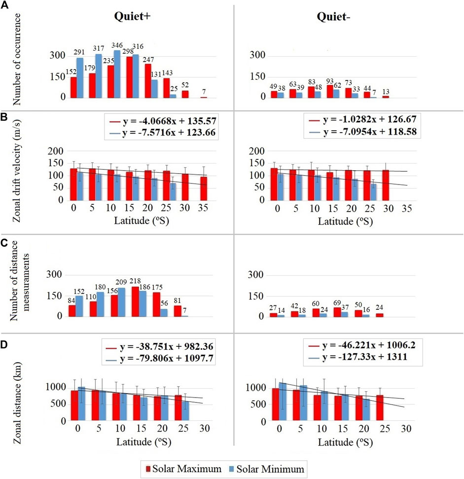
FIGURE 5. EPBs data analysis corresponding to the quiet+ (left side) and quiet− (right side) periods in the solar maximum (red) and the solar minimum (blue). (A) and (C) show the number of EPB occurrences and distance measurements, respectively. (B) and (D) show the mean values of $v_E$ and $d_E$ for 0°S, 5°S, 10°S, 15°S, 20°S, 25°S, 30°S, and 35°S. Error bars represent the standard deviation, and the black lines represent a linear fitting. The regression equations for the solar maximum are represented in red and those of the solar minimum are given in blue.

It should be noted that the EPB occurrence number was smaller during the solar maximum at 0°S, 5°S, 10°S, and 15°S and was higher at 20°S, 25°S, 30°S, and 35°S (Figure 5A, in quiet+). In general, on the quiet− period, we almost notice the same behavior for the quiet+ period concerning the EPB’s number of occurrences for the quiet− period, which is characterized to be higher during the solar maximum (Figure 5A, in quiet−). Figure 5B shows that the $v_E$ value was higher during the solar maximum than the solar minimum, and in both cases, this parameter decreased with the latitude. The $d_E$ value also decreased with the latitude (Figure 5D).

Regarding the zonal drift velocities of EPBs, we noticed that they were higher in the solar maximum than that in the solar minimum. Our results are consistent with the literature. Paulino et al. (2011) studied the EPB zonal drift velocity in a quiet period using airglow images in São João do Cariri (7.4°S and 36.5°W) from September 2000 to April 2007. The authors showed that EPB zonal drift velocities were higher during the solar maximum (∼60 m/s) than those during the solar minimum (∼30 m/s).

3.2 Characteristics of EPBs observed in the disturbed period

In this analysis, 165 days were considered geomagnetically disturbed (Kp >3) at the solar maximum, with 112 days with EPBs (67.9%). Furthermore, 66 disturbed days at the solar minimum with 37 EPB detections (56.1%) were observed. By comparing these results with the geomagnetically quiet period presented in Section 3.1, it can be highlighted that the percentage of EPB occurrences was higher in the geomagnetically disturbed period. In this context, it is important to mention that the number of quiet days (231 days) exceeds the number of disturbed days (165 days).

Figure 6 shows the occurrence rate of EPBs for (a) the solar maximum activity (red scale) and (b) solar minimum activity (blue scale) periods in geomagnetically disturbed conditions (Kp >3). The y-axis shows the month of observation, and the x-axis refers to the time in UT. The black dotted vertical lines are the dusk and dawn terminators at the 350-km altitude. In this figure, it is possible to notice that the highest occurrence rate was between October and March, from 22 UT to 6 UT, 1 h longer than the quiet period. Additionally, we observe three uncommon findings: 1) the pre-dawn EPB occurrence (e.g., on May 2015 at 07 UT, on February 2015 at 08 UT, and on July 2015 at 08 UT); 2) 10% of EPBs occurred on the winter solstice (e.g., May, June, and July 2015); and 3) the EPBs presented longer durations (e.g., on May 2015, EPBs last until 12 UT). In some cases, EPBs crossed the dawn terminator line (e.g., January, February, May, and July 2015, and October 2019).

FIGURE 6

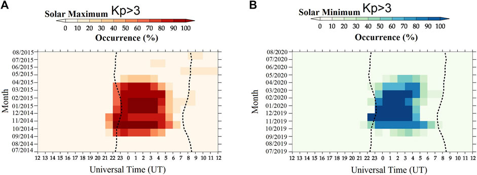
FIGURE 6. Similar to Figure 4, but during the disturbed period (Kp >3). EPB occurrences for the period of (A) solar maximum are represented in red (from July 2014 to July 2015) and those of (B) solar minimum are represented in blue (from July 2019 to July 2020).

The occurrence of pre-dawn EPBs during both solar maximum and solar minimum activities, as depicted in Figure 6, highlights the unusual behavior in their generation. As mentioned previously, during disturbed periods, EPBs can be suppressed, intensified, and generated in unusual times [e.g., pre-dawn (Su et al., 2009; Sripathi et al., 2018; Carmo et al., 2022a; Carmo et al., 2022b)]. The pre-dawn EPBs are supposed to be caused by three different generation mechanisms: 1) PPEF (Su et al., 2009), 2) DDEF (Carmo et al., 2022a; Carmo et al., 2022b), and 3) both PPEF and DDEF (Sripathi et al., 2018). These mechanisms could trigger the RTI and generate EPBs in the pre-dawn hours.

Another characteristic is that 10% of EPB occurrences were in winter during the disturbed periods, which is proportional to the quantity of geomagnetic storm occurrence in winter during the analyzed year. Sobral et al. (2002) also found that the EPB occurrence rate was 10% during winter months. They attributed this behavior to the electric field direction associated with either PPEF or DDEF, which facilitates RTI development (Sobral et al., 2002). In addition, the last unusual occurrence in this analysis, concerning EPBs’ long duration, was attributed to the delay in the emergence of the E-layer after sunrise, as explained by Carmo et al. (2022b).

As mentioned previously, to further investigate the characteristics of EPBs during geomagnetic storms, we divided them according to their disturbance level: weak (left panel), moderate (middle panel), and intense (right panel) of Figure 7. Figure 7A corresponds to the EPB structure’s number of occurrences by fixed geographic latitudes (0°S, 5°S, 10°S, 15°S, 20°S, 25°S, 30°S, and 35°S). Figure 7B shows the mean values of $v_E$ for the eight fixed latitudes. A histogram of the number of measurements available for distance calculations is present in Figure 7C. Each distance measurement requires at least two structures, which results in a lower number of measurements. Figure 7D shows the mean value of $d_E$ for the fixed latitudes. Error bars in this figure represent the standard deviation. The black lines represent a linear fitting, from which a zonal drift latitudinal gradient ($\nabla v_E$) and a zonal distance gradient ($\nabla d_E$) were calculated. Additionally, in this figure, we also provide regression equations.

FIGURE 7

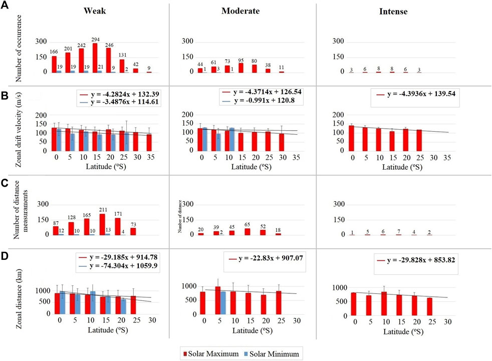
FIGURE 7. Similar to Figure 5, but during the disturbed period (Kp >3). EPB data analysis corresponding to the weak (left side), moderate (middle), and intense (right side) geomagnetic activities in the solar maximum (red) and the solar minimum (blue). (A) and (C) show the number of EPB occurrences and distance measurements, respectively. (B) and (D) show the mean values of $v_E$ and $d_E$ for 0°S, 5°S, 10°S, 15°S, 20°S, 25°S, 30°S, and 35°S. Error bars represent the standard deviation, and the black lines represent a linear fitting. The regression equations for the solar maximum are represented in red and those of the solar minimum are represented in blue.

The number of occurrences (Figure 7A) and measurements (Figure 7C) are higher at the solar maximum than at the solar minimum, where no irregularities were detected at the solar minimum in the intense period. Furthermore, the largest number of observations is between 10°S and 15°S. Figures 7B, D show that $v_E$ and $d_E$ decrease with the latitude in all cases.

Additionally, Sobral et al. (2002) showed that the EPB occurrence rate at the solar maximum is ∼80% higher than that at the solar minimum, which also agrees with the results presented in this study. We can observe quantitative differences, such as the fact that the EPB occurrence at the solar maximum is approximately three times greater than that at the solar minimum. Huang et al. (2002) suggest that the lower occurrences of EPBs detected by the defense meteorological satellite program (DMSP) satellites in the solar minimum may be related to low levels of electric fields in the equatorial ionosphere. The authors showed evidence that the electric fields in the ionosphere and magnetosphere were decreased during the solar minimum. The authors identified three factors that contribute to a higher occurrence of EPBs during the solar maximum: 1) the extension of the effects of the dayside dynamo into the ionosphere after sunset (Eccles, 1998), 2) the uplift of the F-layer in the evening sector caused by gravity waves (Kelley and Larsen, 1981), and 3) the expansion of the system of the Hall current toward lower magnetic latitudes (Wilson et al., 2001). The evidence presented by Huang et al. (2002) supports the results shown in Figure 7.

3.3 Comparison of the characteristics of EPBs at all geomagnetic activity levels

Figure 8 summarizes the result presented in Section 3. This figure shows (Figure 8A) the EPB mean values of the zonal drift velocity $v_E$ and (Figure 8B) the mean values of the zonal distance between two structures $d_E$ for 0°S, 5°S, 10°S, 15°S, 20°S, 25°S, 30°S, and 35°S. This result is presented for each magnetic activity intensity, quiet+ (blue), quiet− (green), disturbed weak (yellow), moderate (red), and intense (dark red) periods. The solid lines correspond to the solar maximum, and the dotted lines, to the solar minimum.

FIGURE 8

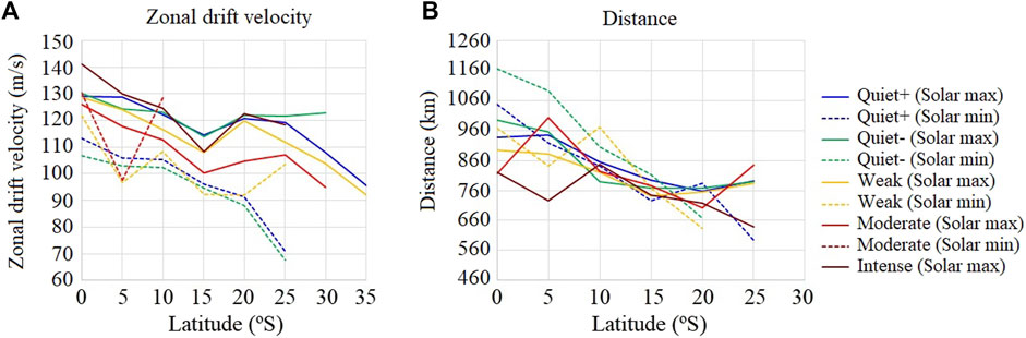
FIGURE 8. (A) EPB zonal drift velocity and (B) distance between EPB structures vs. the geographic latitude. Quiet+, in blue; quiet−, in green; disturbed weak, in yellow; moderate, in red; and intense, in dark red. The solid lines correspond to the solar maximum, and the dotted lines correspond to the solar minimum.

It should be noted that the $v_E$ value presents higher values in the solar maximum than the solar minimum. In general, the $v_E$ value varies between ∼120 and ∼130 m/s in the solar maximum and between ∼100 and ∼108 m/s in the solar minimum at the equatorial region (5°S). At low latitudes, the $v_E$ values are ∼120 m/s in the solar maximum and ∼90 m/s in the solar minimum at a low latitude (20°S). Sarudin et al. (2020) showed that the EPB zonal drift velocity increases with the solar activity. The authors explained that the F-region dynamo is fully activated during the solar maximum as the increased plasma density leads to greater pressure gradients caused by solar heating, resulting in intensified winds. On the other hand, the dynamo is not fully activated due to a lower plasma density during the solar minimum. Consequently, the EPB zonal drift velocity is expected to be greater during the solar maximum, and it is in agreement with this work.

The $d_E$ value of EPBs exhibits similarities between the solar maximum and minimum, from 10°S to 20°S. In general, $d_E$ and $v_E$ values decrease with the increasing latitude. Barros et al. (2018) studied the EPB occurrence from 2012 to 2016, without distinguishing between the geomagnetically quiet and disturbed periods. The authors observed that, on average, EPBs had distances between two consecutive structures of ∼920 km and a zonal drift velocity of ∼123 m/s, which is consistent with the results presented in this work. Moreover, to illustrate the characteristics of EPBs at different levels of magnetic activity, we provide some case examples in Table A1 in the Appendix.

Additionally, Table 2 provides the gradients, $\nabla v_E$ and $\nabla d_E$; the number of measurements for $v_E$ and $d_E$ in the solar maximum; and the minimum for each correspondent of the magnetic activity levels.

TABLE 2

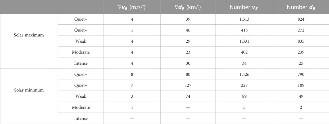
TABLE 2. Gradient ($\nabla {\mathit{v}}_{\mathit{E}}$ and $\nabla {\mathit{d}}_{\mathit{E}}$) and the number of measurements for ${\mathit{v}}_{\mathit{E}}$ and ${\mathit{d}}_{\mathit{E}}$ during the solar maximum and minimum in the quiet+, quiet−, weak, moderate, and intense periods.

Table 2 shows that, on average, the $\nabla v_E$ value was ∼4 m/s per degree in the solar maximum, with the exception of the quiet− period. The $\nabla v_E$ value was ∼7 m/s per degree during the quiet period in the solar minimum, being very different in disturbed periods (3 and 1 m/s per degree). The latitudinal variation presented agrees with the analyses performed by Barros et al. (2018). These variations were associated with latitudinal gradients in the zonal neutral wind velocity (e.g., Sobral and Abdu, 1991; Martinis et al., 2003). We emphasize that between 20°S and 25°S, in Figures 5, 6, 8, there is an increase in $v_E$ at the solar maximum, resulting in the linear fitting falling more slowly than at the solar minimum.

Additionally, the EPB had a smaller latitudinal extension at the solar minimum than the solar maximum. Kepkar et al. (2020) showed that the EPB latitudinal extension is strongly dependent on the PRE, which will cause large magnitudes in the vertical drift of the plasma in periods of the solar maximum. This explains what we see in our results; the apex height that the EPBs reach will be smaller and will, consequently, reach smaller latitudinal distances than the solar maximum.

On average, the $\nabla d_E$ value was ∼33 km per degree in all analyzed cases during the solar maximum. The $\nabla d_E$ value was more pronounced during the solar minimum, with a greater value on the quiet− period (127.3 km per degree). The number of measurements for $v_E$ and $d_E$ were significantly reduced at the solar minimum, except for the quiet+ period, which was 7% larger at the solar minimum than at the solar maximum.

Figure 8A shows that the $v_E$ value in the quiet+ (blue) and quiet− (green) periods presented a similar value, from 0°S to 25°S. In the solar maximum, the $v_E$ value is inversely proportional to the magnetic intensity. The exception behavior is related to the intense disturbance (dark red), which had the highest velocity compared to the others. We believe that during intense events, the PPEF and DDEF are present, which can affect $v_E$, making it difficult to attribute a trend in relation to the magnetic intensity.

In summary, this analysis reveals that all the magnetic activity intensities analyzed, i.e., quiet+, quiet−, disturbed weak, moderate, and intense, exhibited a decrease in both the latitudinal and the zonal drift velocity gradients. More studies are necessary to deepen our understanding of the mechanism driving these observations.

4 Conclusion

This study provides several advances regarding the occurrence and characteristics of EPBs during different solar activity periods and magnetic disturbances levels. These advances are listed as follows:

1. Identification of the peak occurrence period: the highest occurrence rate of EPBs was between October and March, from 22 UT to 05 UT in both the solar maximum and minimum, due to the influence of the geomagnetic declination and geographic latitude of the dip equator in the Brazilian region. The same behavior occurred in quiet and disturbed periods. However, during the disturbed period, it was observed that EPBs lasted 1 h more in their duration (from 22 UT to 06 UT) due to the effects of electric fields from disturbed periods.

2. Duration of EPBs: in the disturbed period, the EPB occurrence rate was 10% in the winter solstice. In the same period, we observe EPBs with a long duration, remaining in the morning (∼12 UT). This behavior is attributed to the geomagnetic storm effects.

3. Higher occurrence of EPBs in the disturbed period: the occurrence of EPBs was 11.8% more at the solar maximum than that at the minimum. This is attributed to electric fields in the ionosphere.

4. Latitudinal extension: during the solar minimum, the latitudinal extension of EPBs was smaller than that of the solar maximum, which can be attributed to the fact that EPBs reached a lower apex height during this period.

5. Higher $v_E$ at the solar maximum: the EPB zonal drift velocity was higher during the solar maximum than that during the solar minimum, and this was attributed to intense winds in this period. On average, the $\nabla v_E$ value was ∼4 m/s per degree during the solar maximum. However, during the solar minimum, the $\nabla v_E$ value was ∼7 m/s per degree during quiet periods and showed a significant difference between disturbed periods (3 and 1 m/s per degree).

6. Pronounced $\nabla d_E$ value at the solar maximum: at the solar maximum, the $\nabla d_E$ value was ∼33 km per degree in all the analyzed cases. However, at the solar minimum, the $\nabla d_E$ value was the most pronounced, with a greater value on the quiet− period (127 km per degree).

Data availability statement

The original contributions presented in the study are included in the article; further inquiries can be directed to the corresponding author.

Author contributions

CC wrote the original draft, provided the accurate data, with the respective investigation, formal analysis, and methodology. CC, DB, and LR contributed to the formal analysis. All authors contributed to the article and approved the submitted version.

Funding

The National Natural Science Foundation of China (42074201 and 41674145) and the International Partnership Program of the Chinese Academy of Sciences (grants 183311KYSB20200003 and 183311KYSB20200017) also provided support for this research.

Acknowledgments

CC and LR thank the China–Brazil Joint Laboratory for Space Weather (CBJLSW), the National Space Science Center (NSSC), and the Chinese Academy of Sciences (CAS) for supporting their postdoctoral fellowship, and JM thanks the CBJLSW/NSSC/CAS for supporting his postdoctoral fellowship. CD thanks the National Council for Scientific and Technological Development (CNPq/MCTI) (grant 303643/2017–0). CF thanks Fundaçao de Amparo a Pesquisa do Estado de São Paulo (FAPESP) (grant 2018/09066–8) and 2019/22548-4), Fundação de Apoio à Pesquisa do Estado da Paraíba, and CNPq/MCTI (grant 301670/2023-4 and 303871/2023-7). CW thanks the CNPq/MCTI (grant 314972/2020-0), DB thanks FAPESP (grant 2021/04696-6), and RS thanks the CNPq/MCTIC (grant 302000/2021–6). SC thanks CAPES/MEC (grants 88887.362982/2019–00 and 88887.694874/2022-00). GP thanks CAPES/MEC (grants 88887.467444/2019-00 and 88887.685060/2022-00). The authors would like to thank the Embrace/INPE Space Weather Program (http://www.inpe.br/spaceweather), the IBGE for providing the satellite data (Rinex) (https://www.ibge.gov.br/geociencias/downloads-geociencias.html), the World Data Center for Geomagnetism, Kyoto, for providing the Dst index (https://wdc.kugi.kyoto-u.ac.jp), the GFZ Potsdam for providing the Kp index (https://kp.gfz-potsdam.de/en/), and Natural Resources Canada for providing the solar radio flux of F10.7 (https://spaceweather.gc.ca/forecast-prevision/solar-solaire/solarflux/sx-5-en.php).

Conflict of interest

The authors declare that the research was conducted in the absence of any commercial or financial relationships that could be construed as a potential conflict of interest.

Publisher’s note

All claims expressed in this article are solely those of the authors and do not necessarily represent those of their affiliated organizations, or those of the publisher, the editors, and the reviewers. Any product that may be evaluated in this article, or claim that may be made by its manufacturer, is not guaranteed or endorsed by the publisher.

References

Aarons, J. (1991). The role of the ring current in the generation or inhibition of equatorial F layer irregularities during magnetic storms. Radio Sci. 26 (4), 1131–1149. doi:10.1029/91RS00473

CrossRef Full Text | Google Scholar

Abdu, M. A., Alam Kherani, E., Batista, I. S., de Paula, E. R., Fritts, D. C., and Sobral, J. H. A. (2009). Gravity wave initiation of equatorial spread F/plasma bubble irregularities based on observational data from the SpreadFEx campaign. Ann. Geophys. 27 (7), 2607–2622. doi:10.5194/angeo-27-2607-2009

CrossRef Full Text | Google Scholar

Abdu, M. A., Batista, I. S., and Bittencourt, J. A. (1981). Some characteristics of spread F at the magnetic equatorial station Fortaleza. J. Geophys. Res. Space Phys. 86 (A8), 6836–6842. doi:10.1029/JA086iA08p06836

CrossRef Full Text | Google Scholar

Abdu, M. A., Batista, I. S., Reinisch, B. W., MacDougall, J. W., Kherani, E. A., and Sobral, J. H. A. (2012). Equatorial range spread F echoes from coherent backscatter, and irregularity growth processes, from conjugate point digital ionograms. Radio Sci. 47 (06), 1–8. doi:10.1029/2012RS005002

CrossRef Full Text | Google Scholar

Abdu, M. A., Batista, I. S., Takahashi, H., MacDougall, J., Sobral, J. H., Medeiros, A. F., et al. (2003). Magnetospheric disturbance induced equatorial plasma bubble development and dynamics: a case study in Brazilian sector. J. Geophys. Res. 108, 1449. doi:10.1029/2002JA009721

CrossRef Full Text | Google Scholar

Ansari, K., Panda, S. K., Kavutarapu, V., and Jamjareegulgarn, P. (2023). Towards mitigating the effect of plasma bubbles on GPS positioning accuracy through wavelet transformation over Southeast Asian region. Adv. Space Res. doi:10.1016/j.asr.2023.04.041

CrossRef Full Text | Google Scholar

Barros, D., Takahashi, H., Wrasse, C. M., and Figueiredo, C. A. O. B. (2018). Characteristics of equatorial plasma bubbles observed by TEC map based on ground-based GNSS receivers over South America. Ann. Geophys. 36, 91–100. doi:10.5194/angeo-36-91-2018

CrossRef Full Text | Google Scholar

Basu, S., Groves, K. M., Basu, S., and Sultan, P. J. (2002). Specification and forecasting of scintillations in communication/navigation links: current status and future plans. J. Atmos. Sol.-Terr. Phys. 64, 1745–1754. doi:10.1016/s1364-6826(02)00124-4

CrossRef Full Text | Google Scholar

Buhari, S. M., Abdullah, M., Hasbi, A. M., Otsuka, Y., Yokoyama, T., Nishioka, M., et al. (2014). Continuous generation and two-dimensional structure of equatorial plasma bubbles observed by high-density GPS receivers in Southeast Asia. J. Geophys. Res. Space Phys. 119 (12), 580. doi:10.1002/2014JA020433

CrossRef Full Text | Google Scholar

Buhari, S. M., Abdullah, M., Hasbi, A. M., Otsuka, Y., Yokoyama, T., Nishioka, M., et al. (2015). Continuous generation and two-dimensional structure of equatorial plasmabubbles observed by high-density GPS receivers in Southeast Asia. J. Geophys. Res. Space Phys. 119 (12), 580. doi:10.1002/2014JA020433

CrossRef Full Text | Google Scholar

Buhari, S. M., Abdullah, M., Yokoyama, T., Otsuka, Y., Nishioka, M., Hasbi, A. M., et al. (2017). Climatology of successive equatorial plasma bubbles observed by GPS ROTI over Malaysia. J. Geophys. Res. Space Phys. 122, 2174–2184. doi:10.1002/2016JA023202

CrossRef Full Text | Google Scholar

Burke, W. J., Gentile, L. C., Huang, C. Y., Valladares, C. E., and Su, S. Y. (2004). Longitudinal variability of equatorial plasma bubbles observed by DMSP and ROCSAT-1. J. Geophys. Res. 109, A12301. doi:10.1029/2004JA010583

CrossRef Full Text | Google Scholar

Carmo, C. S., Denardini, C. M., Figueiredo, C. A. O. B., Resende, L. C. A., Moro, J., Silva, R. P., et al. (2022a). Findings of the unusual plasma bubble occurrences at dawn during the recovery phase of a moderate geomagnetic storm over the Brazilian sector. J. Atmos. Solar-Terrestrial Phys. 235, 105908. doi:10.1016/j.jastp.2022.105908

CrossRef Full Text | Google Scholar

Carmo, C. S., Pi, X., Denardini, C. M., Figueiredo, C. A. O. B., Verkhoglyadova, O. P., and Picanço, G. A. S. (2022b). Equatorial plasma bubbles observed at dawn and after sunrise over South America during the 2015 St. Patrick's Day storm. J. Geophys. Res. Space Phys. 127, e2021JA029934. doi:10.1029/2021JA029934

CrossRef Full Text | Google Scholar

Cherniak, I., and Zakharenkova, I. (2016). First observations of super plasma bubbles in Europe. Geophys. Res. Lett. 43, 137–211. doi:10.1002/2016GL071421

CrossRef Full Text | Google Scholar

Eccles, J. V. (1998). A simple model of low-latitude electric fields. J. Geophys. Res. 103 (26), 26699–26708. doi:10.1029/98ja02657

CrossRef Full Text | Google Scholar

Fejer, B. G., Scherliess, L., and de Paula, E. R. (1999). Effects of the vertical plasma drift velocity on the generation and evolution of equatorial spread F. J. Geophys Res. 104 (A9), 19859–19869. doi:10.1029/1999ja900271

CrossRef Full Text | Google Scholar

Fejer, B. G., de Paula, E. R., González, S. A., and Woodman, R. F. (1991). Average vertical and zonal F region plasma drifts over Jicamarca. J. Geophys. Res. 96 (A8), 13901–13906. doi:10.1029/91JA01171

CrossRef Full Text | Google Scholar

Gonzalez, W. D., Joselyn, J. A., Kamide, Y., Kroehl, H. W., Rostoker, G., Tsurutani, B. T., et al. (1994). What is a geomagnetic storm? J. Geophys. Res. 99 (A4), 5771–5792. doi:10.1029/93JA02867

CrossRef Full Text | Google Scholar

Haerendel, G. (1973). Theory of equatorial spread-F. Report Max-Planck Institute.

Google Scholar

Huang, C.-S., Foster, J. C., Goncharenko, L. P., Erickson, P. J., Rideout, W., and Coster, A. J. (2005). A strong positive phase of ionospheric storms observed by the Millstone Hill incoherent scatter radar and global GPS network. J. Geophys. Res. 110, A06303. doi:10.1029/2004JA010865

CrossRef Full Text | Google Scholar

Huang, C.-S., Foster, J. C., and Sahai, Y. (2007). Significant depletions of the ionospheric plasma density at middle latitudes: a possible signature of equatorial spread F bubbles near the plasmapause. J. Geophys. Res. 112, A05315. doi:10.1029/2007JA012307

CrossRef Full Text | Google Scholar

Huang, C. Y., Burke, W. J., Machuzak, J. S., Gentile, L. C., and Sultan, P. J. (2002). Equatorial plasma bubbles observed by DMSP satellites during a full solar cycle: toward a global climatology. J. Geophys. Res. 107 (A12), SIA 7-1–SIA 7-10. doi:10.1029/2002JA009452

CrossRef Full Text | Google Scholar

Kelley, M. C., Larsen, M. F., LaHoz, C., and McClure, J. P. (1981). Gravity wave initiation of equatorial spread F: a case study. J. Geophys. Res. 86, 9087. doi:10.1029/ja086ia11p09087

CrossRef Full Text | Google Scholar

Kelley, M. C. (2009). The Earth's ionosphere. Elsevier.

Google Scholar

Kepkar, A., Arras, C., Wickert, J., Schuh, H., Alizadeh, M., and Tsai, L.-C. (2020). Occurrence climatology of equatorial plasma bubbles derived using FormoSat-3 ∕ COSMIC GPS radio occultation data. Ann. Geophys. 38, 611–623. doi:10.5194/angeo-38-611-2020

CrossRef Full Text | Google Scholar

Kumar, S. (2017). Morphology of equatorial plasma bubbles during low and high solar activity years over Indian sector. Astrophys. Space Sci. 362, 93. doi:10.1007/s10509-017-3074-3

CrossRef Full Text | Google Scholar

Li, G. Z., Ning, B. Q., Wang, C., Abdu, M. A., Otsuka, Y., Yamamoto, M., et al. (2018). Storm-enhanced development of postsunset equatorial plasma bubbles around the meridian 120°E/60°W on 7–8 September 2017. J. Geophys. Res. Space Phys. 123, 7985–7998. doi:10.1029/2018JA025871

CrossRef Full Text | Google Scholar

Li, Q., Zhu, Y., Fang, K., and Fang, J. (2020). Statistical study of the seasonal variations in TEC depletion and the ROTI during 2013–2019 over Hong Kong. Sensors 20 (21), 6200. doi:10.3390/s20216200

PubMed Abstract | CrossRef Full Text | Google Scholar

Liu, T., Wu, T., Wang, M., Fu, M., Kang, J., and Zhang, H. (2018). “Recurrent neural networks based on LSTM for predicting geomagnetic field,” in 2018 IEEE International Conference on Aerospace Electronics and Remote Sensing Technology (ICARES), Bali, Indonesia, 1–5. doi:10.1109/ICARES.2018.8547087

CrossRef Full Text | Google Scholar

Ma, G., Li, Q., Li, J., Wan, Q., Fan, J., Wang, X., et al. (2020). A study of ionospheric irregularities with spatial fluctuation of TEC. J. Atmos. Solar-Terrestrial Phys. 211, 105485. doi:10.1016/j.jastp.2020.105485

CrossRef Full Text | Google Scholar

Martinis, C., Eccles, J., Baumgardner, J., Manzano, J., and Mendillo, M. (2003). Latitude dependence of zonal plasma drifts obtained from dual-site airglow observations. J. Geophys. Res.-Space 108, 1129. doi:10.1029/2002JA009462

CrossRef Full Text | Google Scholar

Nishioka, A., Saito, A., and Tsugawa, T. (2008). Occurrence characteristics of plasma bubble derived from global ground-based GPS receiver networks. J. Geophys. Res. 113, A05301. doi:10.1029/2007JA012605

CrossRef Full Text | Google Scholar

Ogwala, A., Oyedokun, O. J., Akala, A. O., Amaechi, P. O., Simi, K. G., Panda, S. K., et al. (2022). Characterization of ionospheric irregularities over the equatorial and low latitude Nigeria region. Astrophys. Space Sci. 367, 79. doi:10.1007/s10509-022-04110-0

CrossRef Full Text | Google Scholar

Paulino, I., Medeiros, A. F. D., Buriti, R. A., Takahashi, H., Sobral, J. H. A., and Gobbi, D. (2011). Plasma bubble zonal drift characteristics observed by airglow images over Brazilian tropical region. Rev. Bras. Geofísica 29, 239–246. doi:10.1590/S0102-261X2011000200003

CrossRef Full Text | Google Scholar

Pi, X., Mannucci, A. J., Lindqwister, U. J., and Ho, C. M. (1997). Monitoring of global ionospheric irregularities using the Worldwide GPS Network. Geophys. Res. Lett. 24 (18), 2283–2286. doi:10.1029/97GL02273

CrossRef Full Text | Google Scholar

Pimenta, A. A., Bittencourt, J. A., Fagundes, P. R., Sahai, Y., Buriti, R. A., Takahashi, H., et al. (2003). Ionospheric plasma bubble zonal drifts over the tropical region: a study using OI emission all-sky images. J. Atmos. Solar-Terrestrial Phys. 65 (10), 1117–1126. doi:10.1016/S1364-6826(03)00149-4

CrossRef Full Text | Google Scholar

Rishbeth, H. (2000). “The equatorial F-layer: progress and puzzles,” in Annales geophysicae (Springer), 18, 730–739.

CrossRef Full Text | Google Scholar

Sarudin, I., Hamid, N. S. A., Abdullah, M., Buhari, S. M., Shiokawa, K., Otsuka, Y., et al. (2020). Equatorial plasma bubble zonal drift veloci ty variations in response to season, local time, and solar activity across Southeast Asia. J. Geophys. Res. Space Phys. 125, e2019JA027521. doi:10.1029/2019JA027521

CrossRef Full Text | Google Scholar

Sastri, J. H., Niranjan, K., and Subbarao, K. S. V. (2000). Response of the equatorial ionosphere in the Indian (midnight) sector to the severe magnetic storm of July 15, 2000. Geophys. Res. Lett. 29 (13), 1651. doi:10.1029/2002gl015133

CrossRef Full Text | Google Scholar

Sobral, J. H. A., Abdu, M. A., Batista, I. S., and Zamlutti, C. J. (1981). Wave disturbances in the low latitude ionosphere and equatorial ionospheric plasma depletions. J. Geophys. Res. 86 (A3), 1374–1378. doi:10.1029/JA086iA03p01374

CrossRef Full Text | Google Scholar

Sobral, J. H. A., Abdu, M. A., Takahashi, H., Taylor, M. J., De Paula, E. R., Zamlutti, C. J., et al. (2002). Ionospheric plasma bubble climatology over Brazil based on 22 years (1977–1998) of airglow observations. J. Atmos. Solar-Terrestrial Phys. 64 (12-14), 1517–1524. doi:10.1016/S1364-6826(02)00089-5

CrossRef Full Text | Google Scholar

Sobral, J. H. A., and Abdu, M. (1991). Solar activity effects on equatorial plasma bubble zonal velocity and its latitude gradient as measured by airglow scanning photometers. J. Atmos. Terr. Phys. 53, 729–742. doi:10.1016/0021-9169(91)90124-p

CrossRef Full Text | Google Scholar

Sripathi, S., Banola, S., Emperumal, K., Suneel Kumar, B., and Radicella, S. M. (2018). The role of storm time electrodynamics in suppressing the equatorial plasma bubble development in the recovery phase of a geomagnetic storm. J. Geophys. Res. Space Phys. 123, 2336–2350. doi:10.1002/2017JA024956

CrossRef Full Text | Google Scholar

Su, Y.-J., Retterer, J. M., de La Beaujardière, O., Burke, W. J., Roddy, P. A., Pfaff, R. F., et al. (2009). Assimilative modeling of equatorial plasma depletions observed by C/NOFS. Geophys. Res. Lett. 36, L00C02. doi:10.1029/2009GL038946

CrossRef Full Text | Google Scholar

Sun, L., Xu, J., Wang, W., Yuan, W., Li, Q., and Jiang, C. (2016). A statistical analysis of equatorial plasma bubble structures based on an all-sky airglow imager network in China. J. Geophys. Res. Space Phys. 121, 11,495–11,517. doi:10.1002/2016JA022950

CrossRef Full Text | Google Scholar

Takahashi, H., Costa, S., Otsuka, Y., Shiokawa, K., Monico, J. F. G., Paula, E., et al. (2014). Diagnostics of equatorial and low latitude ionosphere by TEC mapping over Brazil. Adv. Space Res. 54 (3), 385–394. doi:10.1016/j.asr.2014.01.032

CrossRef Full Text | Google Scholar

Takahashi, H., Wrasse, C. M., Denardini, C. M., Padua, M. B., de Paula, E. R., Costa, S. M. A., et al. (2016). Ionospheric TEC weather map over South America. Space weather. 14 (11), 937–949. doi:10.1002/2016SW001474

CrossRef Full Text | Google Scholar

Takahashi, H., Wrasse, C. M., Otsuka, Y., Ivo, A., Gomes, V., Paulino, I., et al. (2015). Plasma bubble monitoring by TEC map and 630 nm airglow image. J. Atmos. Solar-Terrestrial Phys. 130, 151–158. doi:10.1016/j.jastp.2015.06.003

CrossRef Full Text | Google Scholar

Timoçin, E., Inyurt, S., Temuçin, H., Ansari, K., and Jamjareegulgarn, P. (2020). Investigation of equatorial plasma bubble irregularities under different geomagnetic conditions during the equinoxes and the occurrence of plasma bubble suppression. Acta Astronaut. 177, 341–350. doi:10.1016/j.actaastro.2020.08.007

CrossRef Full Text | Google Scholar

Tsunoda, R. T. (1985). Control of the seasonal and longitudinal occurrence of equatorial scintillations by the longitudinal gradient in integrated E region Pedersen conductivity. J. Geophys. Res. 90 (A1), 447–456. doi:10.1029/JA090iA01p00447

CrossRef Full Text | Google Scholar

Tulasi Ram, S., Rama Rao, P. V. S., Prasad, D. S. V. V. D., Niranjan, K., Gopi Krishna, S., Sridharan, R., et al. (2008). Local time dependent response of postsunset ESF during geomagnetic storms. J. Geophys. Res. 113, A07310. doi:10.1029/2007JA012922

CrossRef Full Text | Google Scholar

Vankadara, R. K., Panda, S. K., Amory-Mazaudier, C., Fleury, R., Devanaboyina, V. R., Pant, T. K., et al. (2022). Signatures of equatorial plasma bubbles and ionospheric scintillations from magnetometer and GNSS observations in the Indian longitudes during the space weather events of early September 2017. Remote Sens. 14 (3), 652. doi:10.3390/rs14030652

CrossRef Full Text | Google Scholar

Wan, X., Xiong, C., Wang, H., Zhang, K., Zheng, Z., He, Y., et al. (2019). A statistical study on the climatology of the Equatorial Plasma Depletions occurrence at topside ionosphere during geomagnetic disturbed periods. J. Geophys. Res. Space Phys. 124, 8023–8038. doi:10.1029/2019JA026926

CrossRef Full Text | Google Scholar

Wilson, G. R., Burke, W. J., Maynard, N. C., Huang, C. Y., and Singer, H. J. (2001). Global electrodynamics observed during the initial and main phases of the July 1991 magnetic storm. J. Geophys. Res. 106 (A11), 24517–24539. doi:10.1029/2000ja000348

CrossRef Full Text | Google Scholar

Xiong, C., Park, J., Lühr, H., Stolle, C., and Ma, S. Y. (2010). Comparing plasma bubble occurrence rates at CHAMP and GRACE altitudes during high and low solar activity. Ann. Geophys. 28, 1647–1658. doi:10.5194/angeo-28-1647-2010

CrossRef Full Text | Google Scholar

Zakharenkova, I., and Cherniak, I. (2021). Effects of storm-induced equatorial plasma bubbles on GPS-based kinematic positioning at equatorial and middle latitudes during the September 7–8, 2017, geomagnetic storm. GPS Solut. 25, 132. doi:10.1007/s10291-021-01166-3

CrossRef Full Text | Google Scholar

Appendix

TABLE A1

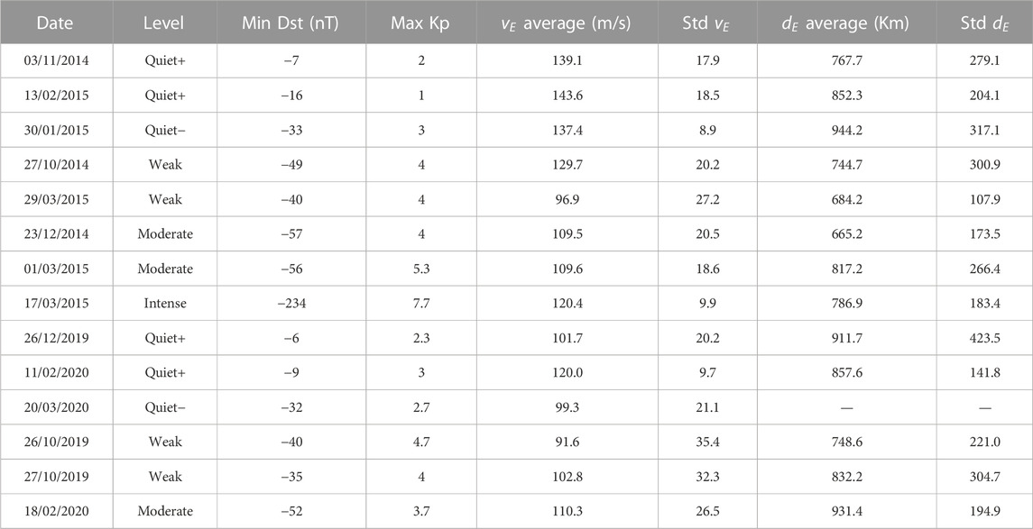
TABLE A1. Examples at different levels of magnetic activity, including the date, magnetic activity level, minimum Dst value for the day, maximum Kp, average of ${\mathit{v}}_{\mathit{E}}$, standard deviation of ${\mathit{v}}_{\mathit{E}}$, average of ${\mathit{d}}_{\mathit{E}}$, and standard deviation of ${\mathit{d}}_{\mathit{E}}$, respectively.