Impacts of Kelvin-Helmholtz billow formation on GNSS radio occultation measurements of sporadic-E

1 Introduction

Sporadic-E (E_s) layers are characterized by unusually large ion densities in the E region of the ionosphere, typically caused by metallic ion convergence through neutral wind shears (Whitehead, 1989; Haldoupis, 2011). These nonuniform, patchy E_s are known to significantly impact High Frequency (HF) skywave propagation (Fabrizio, 2013) and can occasionally reach peak densities capable of reflecting Very High Frequency (VHF) amateur radio (Neubeck, 1996). Additionally, sporadic-E is the leading E-region cause of space-based global navigation satellite system (GNSS) cycle slips (Yue et al., 2016) that impact Low Earth Orbit (LEO) satellite timing. Therefore, understanding the nature of E_s formation and dynamics is vital for many modern technological efforts.

Global sporadic-E monitoring remains challenging, but recent efforts with GNSS radio occultation (RO) have greatly advanced the ability to measure E_s on a truly global scale (Wu et al., 2005; Chu et al., 2014; Arras and Wickert, 2018; Hodos et al., 2022; Yu et al., 2022). Currently, over 20,000 daily occultations are produced from a variety of LEO satellites, with ∼6,500 from Constellation Observing System for Meteorology Ionosphere and Climate (COSMIC-II) covering equatorial and mid-latitudes and ∼16,000 from Spire cubesats which also measure high-latitudes (Wu et al., 2022). While ground-based GNSS sensors have demonstrated the ability to monitor Equatorial Plasma Bubbles (Nishioka et al., 2008; Ansari et al., 2023; Panda et al., 2023), which also significantly impact HF skywave propagation, vertical integration through the ionosphere requires extremely strong sporadic-E layers to produce phase perturbations outside of the sensor noise (Maeda and Heki, 2014; Maeda and Heki, 2015). However, the RO geometry is highly conducive for measuring sporadic-E as the layers essentially act as negative lenses for horizontally propagating GNSS signals (Zeng and Sokolovskiy, 2010). Resulting diffraction patterns can be analyzed using a variety of metrics including phase perturbations (Chu et al., 2014), total electron content (TEC) perturbations (Gooch et al., 2020) and gradients (Niu et al., 2019), and amplitude scintillation (Wu et al., 2005; Arras and Wickert, 2018; Yu et al., 2020).

While GNSS-RO has shown promise in locating sporadic-E layers, extracting additional information such as the peak plasma frequency, foEs, remains challenging due to the unknown horizontal length and vertical thickness of the layers (Gooch et al., 2020; Stambovsky et al., 2021). Previous studies have analyzed the variation in RO signals through E_s layers as strength, length, and vertical thickness are varied while treating the layers as symmetric (Hanning window) lenses (Zeng and Sokolovskiy, 2010; Stambovsky et al., 2021). However, true sporadic-E layers are patchy and billowy, as shown by incoherent scatter radar (ISR) measurements (e.g., Hysell et al. (2009); Hysell et al. (2016)). These turbulent billows are produced through the Kelvin-Helmholtz (K-H) instability, which is a natural result of the wind shear required to form the sporadic-E layers (Bernhardt, 2002). Further, it has been shown that the inclusion of turbulence in multiple phase screen simulations of RO signals through E_s layers significantly improves agreement with scintillation observations (Emmons et al., 2022). Therefore, to accurately extract sporadic-E information from GNSS-RO signals, we must understand both the large- and small-scale dynamics of E_s layers.

An initial attempt to include turbulence in multiple phase screen model simulations was provided in Emmons et al. (2022), where a Kolmogorov power law was used to describe the turbulence following the results of Kyzyurov (2000). While the inclusion of this Kolmogorov turbulence significantly improved the agreement between simulations and observations, the turbulent strength parameter was manually adjusted to improve agreement and was not based on observations or modeled results. Here, we closely investigate the turbulence characteristics by simulating K-H billows in a sporadic-E layer over time and analyzing the resulting power spectrum densities (PSDs). Further, we perform multiple phase screen model simulations through the billowy sporadic-E layer, showing the large variation in GNSS-RO observations possible for a single sporadic-E layer as it develops K-H billows. The resulting turbulence characteristics can then be included in future simulations of RO signals through E_s to improve our understanding between observed RO diffraction patterns and the perturbing sporadic-E layers.

2 Materials and methods

2.1 Two fluid model

A common theory for describing the interaction between a plasma and a magnetic field is the magnetohydrodynamic (MHD) model (Bond et al., 2016). However, the MHD assumptions are not satisfied in the lower ionosphere (Schunk and Nagy, 2009), requiring a more general approach such as the two-fluid plasma model. In the two-fluid model, the ions and electrons are treated separately by a set of electromagnetic fluid equations, retaining both electron inertia effects, displacement currents, and allowing for ion and electron demagnetization (Hakim et al., 2006). The two-fluid approach is necessary for modeling the K-H billow formation due to E-region magnetization differences which impact ion and electron responses to applied forces (such as a neutral wind). For the purposes of this research, the ion density behavior is the primary focus as it displays the most significant dynamic responses throughout the instability process.

Ignoring chemistry, the continuity equation for each species describes the density transport of the plasma in relation to the divergence of the plasma velocity flow:

$\frac{\partial n_s}{\partial t}+\nabla \cdot \left(n_s{\vec{v}}_s\right)=0,(1)$

where n_s and ${\vec{v}}_s$ are the density and velocity terms, respectively, for either ion or electron species s. For simplicity, we only track the metallic ion Fe⁺ and electrons while ignoring the background E-region ions. While this simplifying assumption will need to be addressed in future efforts to improve fidelity, here it provides a first-order approximation to analyze K-H billow dynamics. Coupled to these equations are the velocity field calculations related to pressure forces acting on each species as determined from the momentum equation. Here, we focus on two-dimensional simulations in the $\widehat{x}-\widehat{y}$ plane perpendicular to the magnetic field $\vec{B}$ which points in the $\widehat{z}$ direction. Given the small magnetic declination angle over Arecibo, $\widehat{x}$ is essentially zonal, $\widehat{z}$ is essentially meridional, and $\widehat{y}$ is vertical. Through the diffusion approximation, the steady-state ion velocity can be described by.

${\vec{v}}_s=\frac{1}{1+K_s^2}\left(\begin{array}{cc}\hfill 1\hfill & \hfill K_s\hfill \\ \hfill -K_s\hfill & \hfill 1\hfill \end{array}\right)\cdot {\vec{W}}_s+{\vec{u}}_n,(2)$

${\vec{W}}_s=\frac{1}{m_s{\nu }_{sn}}\left(-\frac{\nabla p_s}{n_s}+m_s\vec{g}+q_s\left[\vec{E}+{\vec{u}}_n\times \vec{B}\right]\right),(3)$

where ${\vec{u}}_n$ is the neutral wind velocity, K_s = ω_c/ν_sn is the ratio of the gyrofrequency to the collision frequency with neutrals, p_s = n_skT_s is the pressure for temperature T_s, $\vec{g}$ is the gravitational acceleration, m_s is the mass, and q_s is the species charge (Schunk and Nagy, 2009). The electric field $\vec{E}=-\nabla \varphi$ is calculated by numerically solving Poisson’s equation at each time step using a finite difference scheme: ∇²ϕ = −∑_sq_sn_s/ϵ₀, which sums over ions and electrons, and ϵ₀ is the permittivity of free space. Here, we assume no external electric fields are present, and the electric fields are created through local charge separation, which affects both ambipolar diffusion and electron and ion drift motions. Combining Eqs 1–3, the steady state momentum equations that describe the velocity of the plasma species are effectively coupled to the continuity equations and solved using a finite difference scheme to determine the temporal evolution of each species’ density. In addition to density, this iterative marching algorithm updates the pressure gradients acting on the plasma that drives the instability perturbations and the velocity flow relating back to the plasma’s momentum. For further information on the model, refer to Bernhardt (2002).

The physical parameters used for the simulations were derived from estimated densities and temperatures at an altitude of 100 km above Arecibo, Puerto Rico on 1 July 2023 at 1800 solar local time. For this time and location, the International Geomagnetic Reference Field (IGRF-13; Thébault et al. (2015)) provides B = 3.5 × 10⁻⁵ T, the Naval Research Laboratory Mass Spectrometer Incoherent Scatter radar (NRLMSIS-2.0; Emmert et al. (2021)) provides an N₂ density of 7.7 × 10¹⁸ m⁻³, the International Reference Ionosphere [IRI-2020; Bilitza et al. (2022)] provides T_n = T_e = T_i = 174 K, and the gravitational acceleration constant is g = 9.5 m/s². From these values, we calculate gyrofrequencies ${\omega }_{c,F{e}^{+}}=60$ rad/s and ω_c,e = 6.1 × 10⁶ rad/s, ion-neutral collision frequency ν_in = 2681 s⁻¹ (Nygren et al., 1984), and electron-neutral collision frequency ν_en = 30, 401 s⁻¹ (Schunk and Nagy (2009), page 109).

An initial density distribution for ions and electrons is given by Equation 4 as referenced in Bernhardt (2002) and projected over a two-dimensional plane shown in Figure 1. This provides the density layer to be evaluated in the two-fluid model from which the K-H billows form. The sporadic-E layer has a vertical thickness of 2.1 km, a horizontal length of 16 km, and a critical peak sporadic-E frequency (foEs) of 4.5 MHz. This short horizontal length of 16 km is implemented to reduce the computation time to simulate the formation of K-H billows. However, the effective length is extended to a more realistic length of 100 km when analyzing impacts on GNSS-RO signals (Section 3).

$n_y=n_o\cosh {\left(y/d\right)}^{\frac{d\cdot V_{oy}}{D_{ay}}},(4)$

where n_o is peak density, d = 700 m, the induced vertical ion drift V_oy = 0.7 m/s, and the vertical ambipolar diffusion coefficient D_ay = 19.3 m²/s (Bernhardt, 2002). Eqs 5, 6 provide the formulations for the $\widehat{x}$ and $\widehat{y}$ a priori defined velocity components, respectively, that trigger the instability process. Figure 2 shows the projection of these velocity distributions onto the physical dimensions of the density map. The sinusoidal distribution creates two initial perturbations along the vertical axis. The zonal flow creates opposing forces along the horizontal direction, interacting with the vertical perturbations to generate instabilities in the metallic ions.

$u_x=u_{ox}\tanh \left(\frac{y}{d}\right),(5)$

$u_y=u_{oy}\sin \left(\frac{\pi }{2}x\right),(6)$

where x specifically describes the sinusoidal length of the perturbation, $-\frac{\pi }{2}\le x\le 2\pi$, to be projected over the horizontal axis, and the initial velocities defined as u_ox = 100 m/s and u_oy = 5 m/s. From the N₂ density, gravitational constant, horizontal perturbation scale d, and the initial horizontal velocity, a Richardson number of 0.09 is calculated, indicating a positive K-H growth rate (Bernhardt, 2002).

FIGURE 1

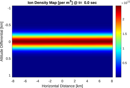
FIGURE 1. Initial density distribution of the sporadic E-layer with a vertical thickness of 2.1 km, a horizontal length of 16 km, and an foEs of 4.5 MHz. This relatively short horizontal length was used to reduce computation time.

FIGURE 2

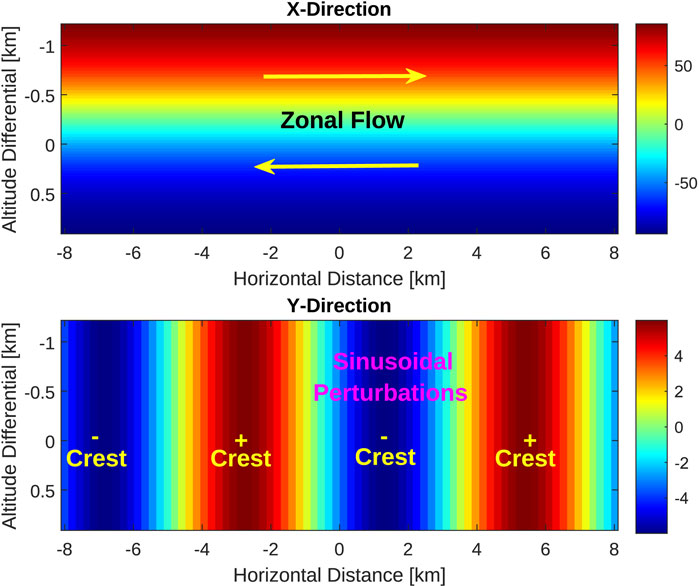
FIGURE 2. Initial velocity (m/s) perturbation distributions in the (top) horizontal x direction, and (bottom) vertical y directions.

The initial discretization parameters that define the domain are 75 grid samples mapped over the 2 km km region with a time step of unity. The sparseness of the simulation parameters is required to holistically model the gradual changes in the K-H billows within a reasonable duration of simulation time. In this particular research effort, using a 12th generation Intel (R) Core (TM) i3 3.30 GHz processor, a simulation run time of $\sim 15$ minutes was achieved.

Figure 3 shows the temporal evolution of the metallic ion density layer. The corresponding velocity vector field maps are shown in Figure 4. The initial stage of the simulation demonstrates the shear flow’s gradual interaction with the set of sinusoidal crests as the velocity field dominates in the x-direction. Vertical motions generate billows in the initial stages that gradually decrease peak density magnitudes, observed through ∼300 s. Throughout the process, gravity and pressure gradients influence the shaping of these uniform billows as they rotate about their central axes. Initially, the plasma is in equilibrium because the pressure gradients are acting equally towards each other from top to bottom and left to right, compressing/converging the plasma. The initial gravitational force applied downward ($-\widehat{y}$-direction) against the plasma layer pushes this layer in the same direction as the force applied. Coupled with the initial sinusoidal perturbation in the plasma, the pressure components are no longer in equilibrium and are now under the influence of the momentum driven by the predefined velocity perturbation components along the $\widehat{y}$-direction pointing up (along the positive crest) and down (along the negative crest) throughout the layer. The change in plasma equilibrium gradually takes the form of a rotation as the dominant zonal drifts caused by the horizontal velocity (upper and lower half of the layer experiencing oppositely directed velocity components) continue to interact with the lesser vertical velocity components and gravitational force. A shear flow begins to grow through this interaction and manifests itself within the pressure gradients as the transport of density vortices shown in Figure 3 strongly corresponds to the points where the crest in the sinusoidal perturbation changes from positive to negative, pointing in opposite directions from top to bottom (out of equilibrium). Additionally, the horizontal components of the pressure gradients point oppositely (the bottom half of the layer is to the right, and the top half of the layer is to the left).

FIGURE 3

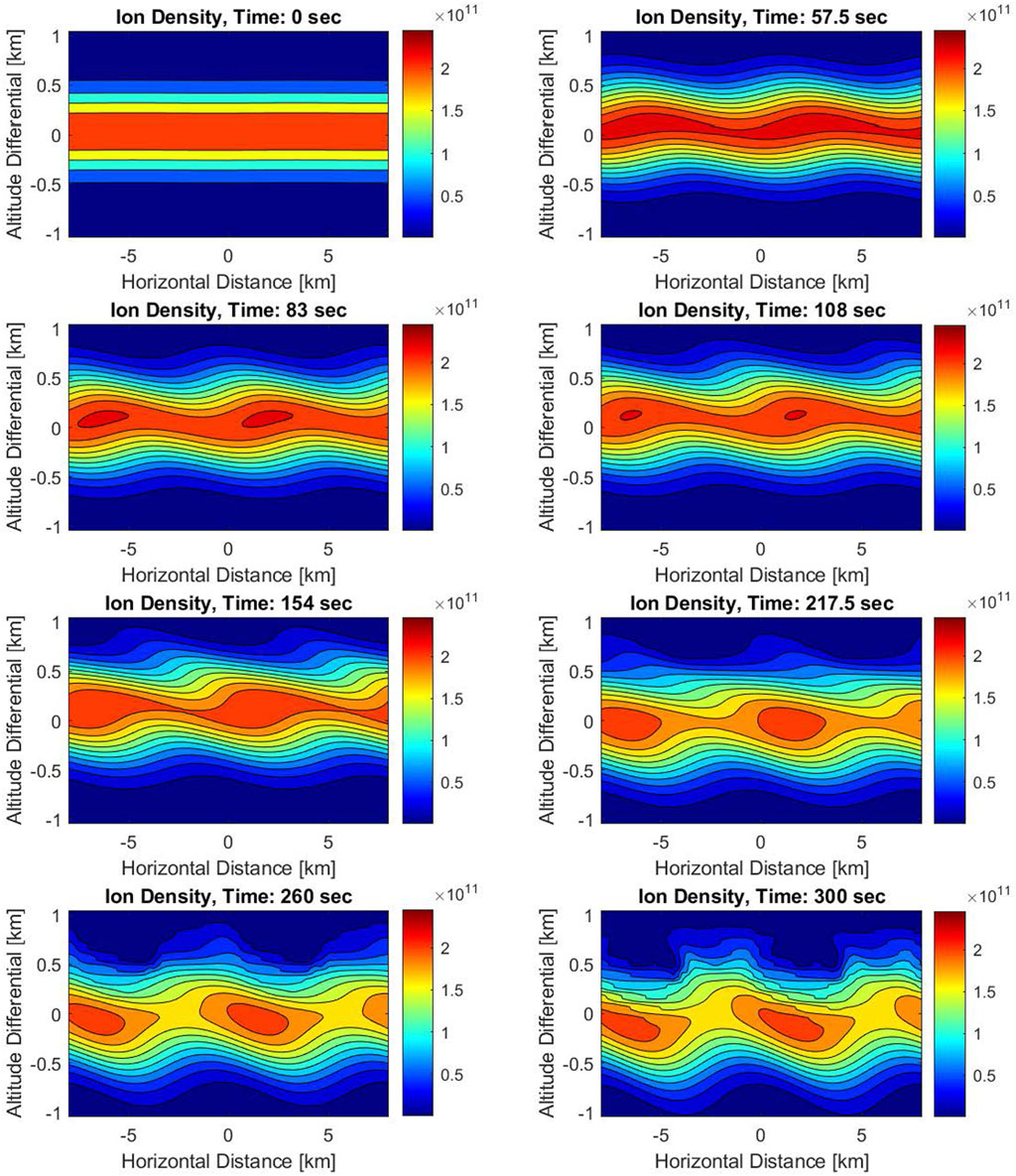
FIGURE 3. Time evolution of the metallic ion density (1/m³) K-H billows. Note the layer widening in the vertical direction and overall reduction in peak ion densities as the billows evolve.

FIGURE 4

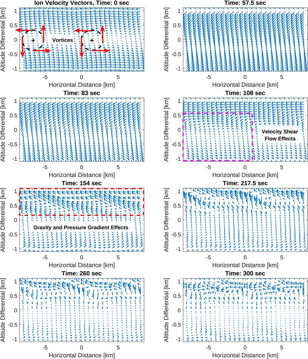
FIGURE 4. Ion velocity vector evolution influencing the ion densities, illustrating the direction of the ion flow in which two layers form from the initial perturbation and move in opposite directions, creating characteristic shear flow effects that influences the turbulent K-H motion.

In comparison to the simulations from Bernhardt (2002), key similarities are observed in the formation of these two distinct billow vortices from the shear flow effects of the velocity fields on the E_s layer. However, in the two-fluid model used in this current paper, only a 300 s time duration is applied instead of 700 s from Bernhardt (2002) to allow the shear flow effects to manipulate the density billows as asymmetries develop. A key reason for the 300 s time restriction is that the shear flow continues to influence these density billows until the classic K-H hook forms between the high- and low-density layers. The K-H hook dominates and eventually masks out the low-amplitude billows, in contrast to the Bernhardt (2002) in which the quasi-periodic density billows became more stable beyond 300 s, eventually achieving a steady state. Although the key governing two-fluid continuity and momentum equations are applied in both Bernhardt (2002) and this paper, additional consideration of differences in the results lies in the application of these equations. Bernhardt (2002) uses a three-dimensional frame in which the gravitational component is applied along the $\widehat{z}$-axis and the plasma velocities are simulated in all three dimensions. This is translated through calculations of the mobility tensor that describes the electron and ion transport and subsequent calculations of the forces applied on each species. This current paper formulates the problem in a two-dimensional construct in which the lateral velocity components are reduced to two dimensions ($\widehat{x}-\widehat{y}$ plane) and the gravity component ($-\widehat{y}$-directed) resides within this plane. With fewer dimensions, the interaction between each of the applied forces on the plasma density is expected to differ during the simulation process. Regardless of these observed differences between the models, the formation of the K-H hook is expected after the density layer experiences prolonged shear flow effects. This observation at later times during the simulation run of this current model validates that the intended physical process is ultimately achieved.

The following section applies the ion density map generated from the two-fluid model to evaluate the scattering characteristics of the propagation channel in a GNSS radio occultation geometry.

2.2 Phase screen pulse coherence model

The concept of the multiple phase screen model for the GNSS radio occultation problem, as illustrated in Figure 5, begins with an understanding of the propagation method for the electric field, $\vec{E}$, across the K-H billow perturbed medium. Following Levy (2000), to simplify the numerical simulations of wave propagation through the sporadic-E layer to the LEO satellite measurement plane, we first reduce the simulation to the scalar electric field, E, ignoring the polarization. From this, the wave equation can be recast to the Helmholtz equation through the assumption of a harmonic time dependence, $E\sim \exp \left\{-i\omega t\right\}$ for the angular frequency ω:

$\frac{{\partial }^{2}E}{\partial y^2}+\frac{{\partial }^{2}E}{\partial x^2}+k_0^2{n}^2\left(x,y\right)E=0,(7)$

where k₀ is the free space wavenumber 2π/λ_L1, and $n=\sqrt{1-f_p^2(x,y)/f_{L1}^2}$ is the refractive index for a non-magnetized plasma with plasma frequency f_p and signal frequency f_L1 (Jackson, 1999). The phase screen propagation method requires a slow-varying amplitude envelope assumption of the Helmholtz equation to obtain the parabolic wave equation, thereby allowing for a marching solution instead of solving for a full spatial grid at each time step. This is especially desirable for modeling propagation distances over long distances, as presented with the GNSS radio occultation geometry, rather than using full wave techniques that strain computational resources.

FIGURE 5

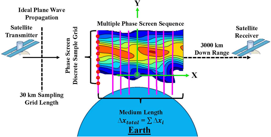
FIGURE 5. GNSS radio occultation geometry used in a multiple phase screen propagation model.

Eq. 8 shows the resulting parabolic wave equation from the slow-varying envelope assumption in which the reduced scalar electric field, $\xi =E\exp \left(-i{k}_{0}x\right)$, is directed along the vertical y-direction and propagates in the horizontal x-direction. Here, the wavelength must be significantly smaller than the transverse scale length along the propagation path, which allows us to drop the ∂²ξ/∂x² term. This condition is certainly satisfied in this research effort given that the frequency of evaluation for GNSS is in the L-band, yielding a wavelength of 19 cm relative to a scale length on the order of thousand(s) of kilometers for GNSS radio occultation measurement of the downrange received field.

$\frac{{\partial }^2\xi }{\partial y^2}+2i{k}_0\frac{\partial \xi }{\partial x}+k_0^2\left[n^2\left(x,y\right)-1\right]\xi =0.(8)$

This parabolic form allows forward-marching solutions because of the first order derivative in x, which only requires an initial condition that can be propagated forward throughout the simulation. Numerical propagation is usually accomplished using a technique such as the Fourier split-step method, which propagates between discrete phase positions x_i using a Fourier transform with respect to the vertical direction $\widehat{y}$ combined with a simple free-space propagation solution in Fourier-space. After propagating to the next x_i+1 location, an inverse Fourier transform is applied and the spatially dependent phase is added to the reduced scalar electric field ξ. This process is repeated until the signal reaches the LEO satellite measurement plane at a distance of 3,000 km from the sporadic-E layer. The reduced electric field ξ is then converted to the electric field E, providing information on the amplitude and phase of the signal as a function of altitude in the measurement plane. The diffractive effects of sporadic-E layers on GNSS-RO signals can be calculated using this approach, providing a physics-based method for reconstructing complex RO measurements. Further details on the derivation and numerical techniques can be found in Knepp (1983); Levy (2000); Rino (2011).

The next key concept of the propagation model is that, for a single uniform planar wave propagating through the K-H billow channel, a sequence of phase screens are required to account for these variations in the density perturbations that induce spatially dependent phase perturbations to the propagating plane wave. Each phase screen in sequence along the propagation path acts as a lens that focuses or diverges the concentration of energy in the perturbing electric field. The phase screen calculation is based on an optical path length calculation over a certain thickness of the medium, compressing the density area down to a thin screen of discrete phase samples. The conversion from density to phase can be applied using this concept:

$\begin{array}{ll}\hfill {\varphi }_i\left(x_i,y_j\right)& =\left(\frac{2\pi }{\lambda }\right)n\left(x_i,y_j\right)\mathrm{\Delta }{x}_i\hfill \\ \hfill {\varphi }_{\mathit{total}}\left(y_j\right)& ={\displaystyle \sum _{i=0}^N}{\varphi }_i\left(y_j\right),\hfill \end{array}(9)$

where i denotes the particular screen realization in the propagation direction, j designates the transverse (vertical) index, λ is the wavelength of the propagating field, n (x_i, y) is the refractive index of the propagation channel, and Δx_i is the thickness of the particular portion of the medium that is being compressed to a screen. For the purposes of this research, the total phase variation of the medium is reduced to a singular phase screen (Eq. 9) to further reduce the computation time of the received electric field realizations over the bandwidth of the GNSS pulses.

After the received electric field at the LEO measurement plane is calculated numerically, the resulting signal perturbation as a function of altitude can be analyzed. To quantify the scintillation caused by the sporadic-E layer, a 2.2 km sliding window is used to calculate the amplitude-based S₄ and phase-based σ_ϕ.

$S_4\left(y\right)=\sqrt{\frac{⟨{\mathrm{E}}^4\left(y\right)⟩-{⟨{\mathrm{E}}^2\left(y\right)⟩}^2}{{⟨{\mathrm{E}}^2\left(y\right)⟩}^2}},(10)$

${\sigma }_{\varphi }\left(y\right)=\sqrt{⟨{\varphi }^2\left(y\right)⟩-{⟨\varphi \left(y\right)⟩}^2},(11)$

where E is the signal amplitude, ϕ is the signal phase, ⟨ ⟩ denotes the average over a 2.2 km sliding window, and y is the altitude (Briggs and Parkin, 1963). The 2.2 km window corresponds to the vertical distance covered by the RO tangent point during a 1-s interval.

In this study, we rely on simulations for our materials and methods, with a primary focus on the K-H billow perturbations to GNSS-RO signals. K-H billows have been experimentally observed in sporadic-E layers using incoherent scatter radars (ISRs; Hysell et al. (2012); Hysell et al. (2016)), qualitatively matching the simulations of Bernhardt (2002). However, concurrent measurements of K-H billows from both ISR and GNSS-RO have yet to be compared, likely due to the precise timing required to simultaneously observe the billows with both. While this study does not provide concurrent measurements, we provide a framework for analyzing K-H billow perturbations to GNSS-RO signals and qualitatively compare the RO simulations against sample measurements of sporadic-E.

3 Results

3.1 Power spectral density

Figures 6, 7 show the power spectrum distributions in the $\widehat{x}$ and $\widehat{y}$ directions calculated from autocorrelations of phase samples within the density maps of Figure 3. Autocorrelation is the initial step to creating a phase screen from the density map, as it forms a Fourier transform pair with the power spectrum. The densities along the propagation path must be converted to phase via the optical path length that spans the propagation distance along the density map. Autocorrelation amounts to establishing an intended direction to propagate and taking a Fourier transform of all the phase samples to establish their complex values, followed by multiplying these values by a complex conjugate version of itself (the correlation component). This is considered an autocorrelation because a copy of the original vector is applied to this process. The multiplication of these two components reveals the phasor difference between two vectors, measuring the phase rotation in the complex plane (frequency domain), or equivalently, the displacements caused by the perturbations in the spatial domain. The inverse Fourier transform is taken to convert the result back into the spatial domain.

In Figure 6, the autocorrelation calculation of the power spectrum is along the length of the layer for each time sequence, inherently biased by the consistency of the density gradients along the sampling path. In the analysis of the power spectrum distributions with respect to each propagation path, a low frequency point is selected where the peak power magnitude occurs, and a high frequency point is selected at the beginning of the power spectrum’s noise floor. The combination of these two points allows for a slope calculation to characterize the rate of energy decay caused by the neutral wind driven turbulence. This slope is used as an indication of the decay rate from large-scale size turbulence to small-scale sizes. A steeper slope along the power spectrum indicates that beyond the point of the peak power spectrum, there is very little correlation in the smaller perturbations, in which the smaller scale sizes have a minimal cumulative effect along the propagation path. A gradual slope indicates that the smaller irregularities have a greater cumulative effect from the autocorrelation of these phase samples compared to the large-scale irregularities that may coexist.

FIGURE 6

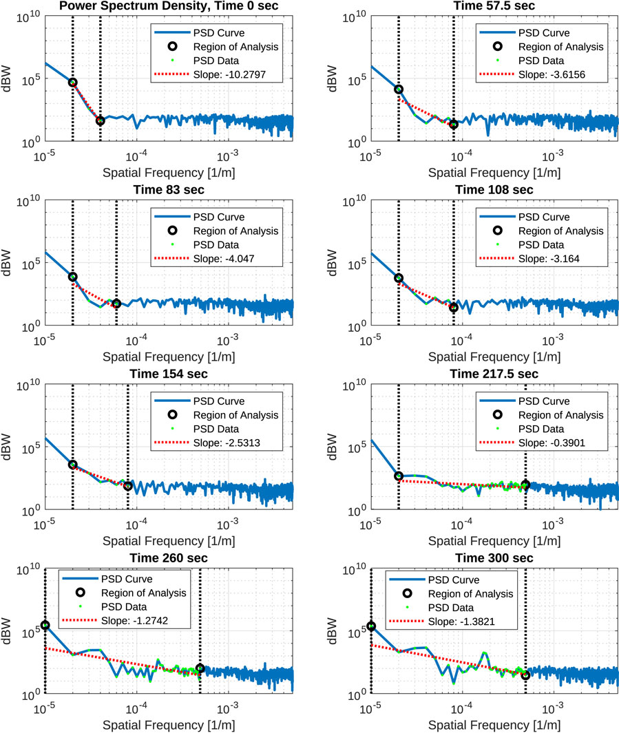
FIGURE 6. Power Spectrum Density distribution over the horizontal (left-to-right) direction along the propagation path of the ion density layer with foEs = 4.5 MHz. For reference, the Kolmogorov power spectrum has a slope of −3.

Observing the power spectrum density distributions along the 100 km horizontal propagation path, the spectral slope magnitudes in the decay profile between selected low and high frequency points is at a peak slope decay initially, prior to any billow formation. The consistency in the E_s density layer along this path is at its greatest, contributing to a stronger correlation of the phase samples and conversely translating to a power spectrum roll-off over a narrow spatial frequency range. As the billows form, the E_s layer loses this consistency, varying more significantly over time along the horizontal path, and the spatial frequency range of the power spectrum roll-off tends to broaden prior to achieving the noise floor. Minor secondary peaks can be observed in the power spectrum roll-off, initially forming at 217.5 s and growing through the remaining time. These peaks indicate constructive accumulation of the phase power spectrum over the corresponding spatial scale sizes (large-scale sizes corresponding to small spatial frequencies).

These initial power spectrum distributions appear to be similar to the analytic Gaussian spectra that are typically associated with predicting the effects of large-scale irregularities (Stambovsky et al., 2021). As time evolves, the density of the billows dimishes and their circular regions of peak intensity become smaller, translating to a gradual decline of the phase power spectrum along the increase of the spatial frequency scale. A linear power roll-off becomes more prominent, consistent with the theorized power law (Kolmogorov) spectrum often applied in phase screen modelling for generalizing large-scale ionospheric turbulence with inclusion of small-scale size irregularities (Kyzyurov, 2000; Emmons et al., 2022).

While not applicable to the RO geometry, the vertical PSD may be useful for ground-based GNSS and radio frequency (RF) beacon sensors. In Figure 7, the autocorrelation calculation of the power spectrum is shown along the vertical thickness of the layer for each time sequence. The autocorrelation calculation of the power spectrum along the vertical thickness of the layer (approximately 2 km) results in a moderately lower peak phase power spectrum and a lower spectral slope in general compared to the results of Figure 6. Initially, the symmetry in the E_s layer along the vertical path creates a cancelation of the autocorrelated phase that contributes to a very low phase power spectrum. The analogous effects observed in the horizontal path cases are also present in the vertical path cases, in which the spatial frequency window widens over the phase power spectrum roll-off prior to achieving the noise floor. The distinct secondary peak features previously observed in the later time stamps of the phase power spectra in Figure 6 are not apparent in Figure 7, due to fewer unique density variations (more symmetry in the density layer) along the vertical axis, despite the presence of billows.

FIGURE 7

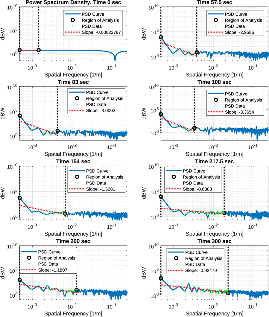
FIGURE 7. Power Spectrum Density distribution over the vertical (bottom-to-top) direction along the thickness of the ion density layer. For reference, the Kolmogorov power spectrum has a slope of −3.

3.2 Multiple phase screen model

To calculate the GNSS signal’s electric field amplitude and phase at the LEO satellite measurement plane for the RO geometry, a multiple phase screen model is implemented. This phase screen model accounts for the sporadic-E layer’s ion density enhancement by spatially adjusting the refractive index, which is a function of the plasma density. The GNSS signal is treated as a plane wave before encountering the sporadic-E layer that adds a spatially varying phase to the signal, which is then propagated 3000 km to the LEO satellite measurement plane by numerically solving Eq. 8. At the measurement plane, the signal’s amplitude and phase perturbations can be analyzed as a function of altitude.

The phase screen model parameters consisted of a vertical grid length of 14 km at a sample size of 3000, and a carrier frequency of GPS L1 band: 1575.42 MHz. The optical path length thickness of the propagation channel applied for the phase screen calculation is 100 km in length. The 100 km medium length is a necessary expansion of the 16 km density map from the two-fluid model to achieve the median sporadic-E length as observed by GNSS measurements in Japan (Maeda and Heki, 2015). The original density map (i.e., density maps in Figure 3) is scaled in length during the optical path length-to-phase conversion (Eq. 9) in which Δx_i is determined by dividing the 100 km length by the 76 samples from the original density map. Once the total phase is determined from the 76 × 76 density map, linear interpolation is used to expand the number of samples to a 3000 × 3000 array to improve fidelity of the perturbation gradient variations and to create a smaller spatial index for the phase screen to adequately capture small-scale perturbation effects. This array is compressed to a 3000 × 1 dimension when calculating the phase screen from the density map’s optical path length along the GNSS-RO path.

Throughout each simulation,4.5 MHz foEs is consistently applied for the initial intensity to clearly show the variation over time. While this 4.5 MHz layer is stronger than the mean foEs of ∼3.0 MHz (Yu et al., 2020), the stronger layer helps to highlight the large changes in GNSS signal perturbation over time during K-H billow formation. The following results demonstrate the scattering characteristics of the received GNSS signal that propagated through the temporally evolving K-H billows. It is important to note that the evaluation of the received field is 3,000 km downrange from the end of the density layer (the compressed screen) for the RO geometry. The sequence of plots in Figure 8 shows the characteristic “U” shape in the amplitude response (Zeng and Sokolovskiy, 2010) that gradually decays as the ion density is diminished and spread vertically, creating a thicker and weaker lens. Within the first minute, as the K-H billows begin to form, the sporadic-E layer spreads vertically and reduces the severity of focusing observed for the initial symmetric layer. However, the symmetric “U” shape amplitude profile remains mostly intact for the first few minutes until the K-H billows are fully developed, producing strong asymmetries in the ion densities that result in weaker, asymmetric diffraction patterns for the RO signals.

FIGURE 8

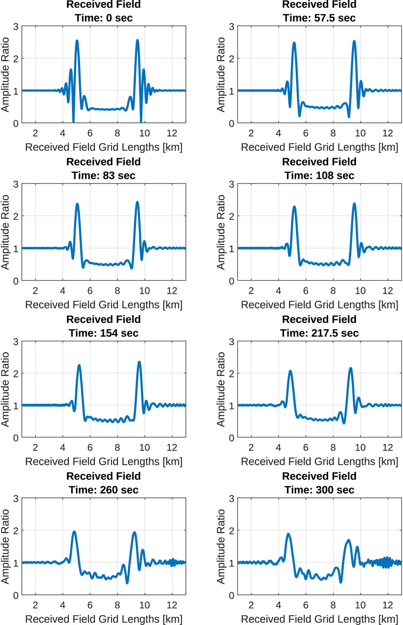
FIGURE 8. GNSS signal amplitudes (E) at the LEO measurement plane over the time lapse of the K-H billows using an initial foEs of 4.5 MHz and a sporadic-E horizontal length of 100 km. Note the decay and asymmetry of the characteristic “U” shape pattern as the billows evolve.

Relating these results to their corresponding power spectrum distributions from Figure 6, the loss of symmetry in the received field after ∼200 s corresponds to a flatter power spectrum with a slope magnitude below 1.5, indicating that the large-scale structures are diminishing in place of small-scale structures from the K-H billows. This observation further supports the notion that at higher wavenumbers, the smaller scale size structures produces significant angular scattering, contributing to the interference patterns observed in the received field at 3,000 km down range. At the other captured times, the characteristics of the spectral slope in the power spectrum dominate the observed intensity of the received field fluctuations, in which the steeper decay in the cascading of energy corresponds to a greater diffraction intensity because the smaller-scale perturbations have either not taken form or are not strong enough to sustain the phase power over the spatial frequency spectrum.

The corresponding phase variations in the received field shown in Figure 9 display subtle asymmetries throughout much of the simulation duration. Spatial asymmetries in the phase screen are a key contributor to the asymmetries observed in the amplitude and phase of the received field. The greatest observed variation is the peak magnitude of the phase change from −0.4 m initially to −0.6 m after the first minute. This increase in the magnitude of the phase perturbation may seem counterintuitive, but it is an artifact of the strong focusing caused by the initial sporadic-E layer that produces significant phase scintillation, as seen in Figure 9 at the edges of the phase perturbation. As the layer expands and develops asymmetries during K-H billow formation, the severity of focusing is decreased, which reduces the amount of phase scintillation, resulting in a larger phase perturbation. For times after the first minute, the phase perturbation is reduced and subtle asymmetries develop as the K-H billows evolve. These results are also consistent with the behavior observed in the power spectrum plots of Figure 6. As the peaks of the power spectrum recede along the spatial frequency spectrum over time, decreasing in spectral slope, the optical path length of the propagation channel will shorten as the density perturbations weaken, minimizing the observed phase variations.

FIGURE 9

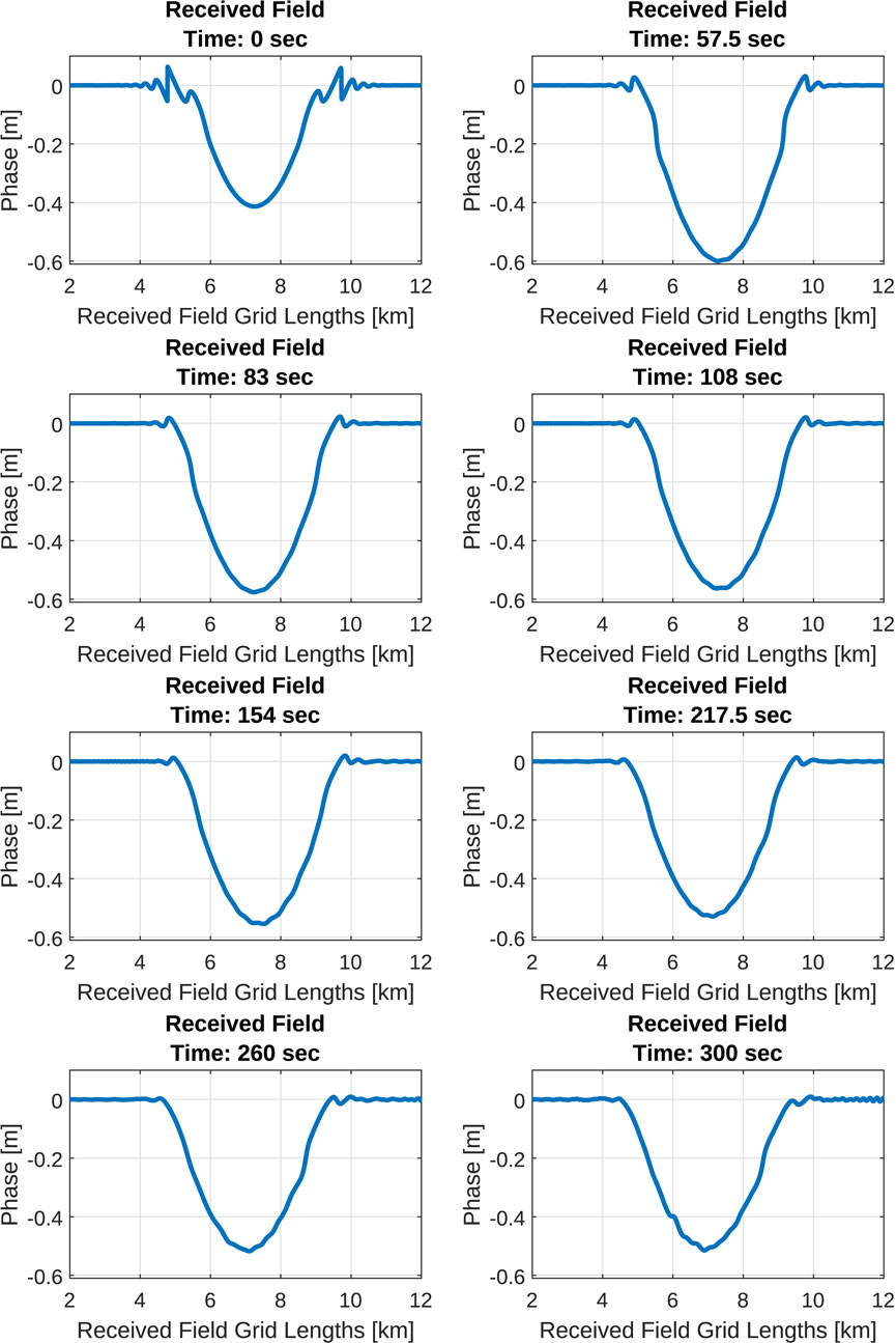
FIGURE 9. GNSS signal phases (ϕ) at the LEO measurement plane over the time lapse of the K-H Billows using an initial foEs of 4.5 MHz and a sporadic-E horizontal length of 100 km. Note the subtle asymmetries produced by billow formation.

Figures 10, 11 show the maximum amplitude and phase scintillations, respectively, over the entirety of the GNSS radio occultation propagation to the LEO measurement plane calculated using Eqs 10, 11. At 3,000 km, the peak S₄ magnitude decreases over time as the K-H billows form and evolve. This reduction in S₄ is caused by an expansion in the vertical lens thickness for the sporadic-E layer in addition to imperfections caused by spatial asymmetries.

FIGURE 10

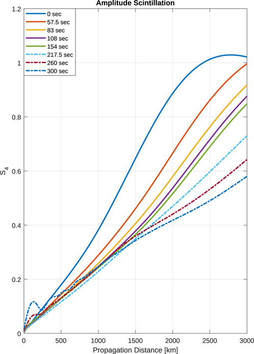
FIGURE 10. Peak amplitude scintillation (S₄) distributions as a function of propagation distances during K-H billow formation. Note the general decrease in magnitude as the billows form and evolve.

FIGURE 11

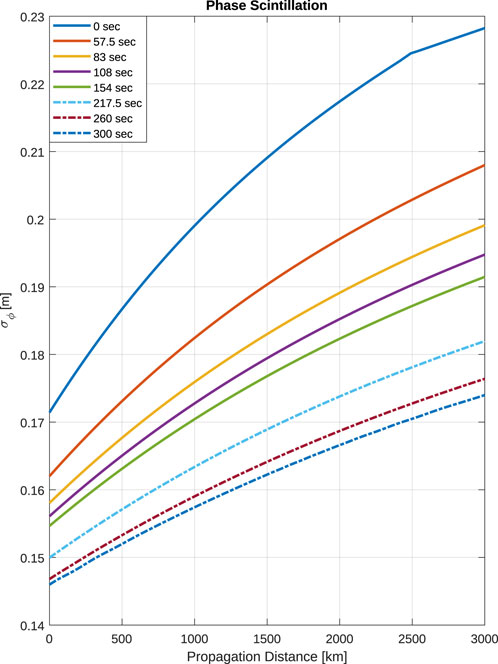
FIGURE 11. Peak phase scintillation (σ_ϕ) distributions as a function of propagation distance during K-H billow formation. Note the general decrease in magnitude as the billows form and evolve.

Similar behavior is observed for the phase scintillation, σ_ϕ, which show peak values of 0.23 m at the LEO measurement plane (3,000 km) for the initial sporadic-E layer (Figure 11). As K-H billows form, phase scintillation is reduced following the temporal trends in Figure 9. This reduction in σ_ϕ is a consequence of lens imperfections and expansion, which reduces the focusing severity.

4 Discussion

The two-fluid simulations of K-H billow formation presented here are very similar to the simulations outlined in Bernhardt (2002), which are, in turn, qualitatively similar to the ISR observations shown in Hysell et al. (2016). This billow formation transforms the strong, thin sporadic-E layers into wider, more turbulent layers, and this transformation has a large impact on the GNSS-RO signals used to monitor these layers.

Recently, Emmons et al. (2022) found that the inclusion of Kolmogorov turbulence in the layers helped to significantly improve agreement with observations, mostly due to vertical asymmetries that are more physically realistic than the strong focusing symmetric lenses. In relation to the Kolmogorov spectrum for sporadic-E outlined in Kyzyurov (2000), the power spectra simulated from the K-H billow evolution over time reveal more significant slope decay magnitudes along the GNSS-RO path in many cases, demonstrating that the large-scale features of the structure are dominant over the small-scale features, particularly early in the simulation. As the simulation progresses in time, the billows shrink spatially, density gradients become less consistent, and perturbations weaken, causing the spectral slope to become more shallow, ultimately converging to a PSD flatter than the Kolmogorov spectrum. The relationship between this variation in the scale size and the corresponding effect on the power law slope is perhaps captured more definitively in the vertical direction as the billows grow, shrink, and evolve to the K-H hook. The behavior of the power law slope corresponds more directly to these variations in density observed along the vertical optical path length compared to the GNSS-RO path, making the slope of the power law behavior more difficult to predict in time. These results emphasize the crucial application of the two fluid model to capture the K-H billow structure characteristics at various phases in time that otherwise cannot be generalized using an independent, traditional Kolmogorov phase screen framework that follows a particular power law slope.

Here, we show that a single E_s layer can result in a wide variety of diffraction patterns due to K-H billow formation. Practically, this indicates that most of our current techniques for estimating E_s intensities (i.e., foEs or fbEs) that rely on either the amplitude scintillation (e.g., S₄ index for the Yu et al. (2020) technique) or phase perturbations (e.g., TEC perturbations for the Gooch et al. (2020) technique) could result in large variations for the intensity estimates over a relatively short amount of time. As displayed in Figures 8, 10, the large variations in amplitude profiles over the 300 s during billow formation result in a large variation of S₄ values, which would in turn result in large variations in foEs estimates from the Yu et al. (2020) conversion formula: (foEs-1.2)² = 13.62×S_4,max.

Further, many studies have used ionosonde observations as ground truth for comparison with RO observations of sporadic-E layers (Arras and Wickert, 2018; Niu et al., 2019; Gooch et al., 2020), which requires a tangent point distance and time constraint for comparison. For example, Gooch et al. (2020) compared ionosonde and RO observations within 150 km and 30 min. However, from the results shown here (and in ISR observations: e.g., Hysell et al. (2016)), K-H billows can significantly affect the E_s characteristics and resulting RO observations within a short ∼5 min window. In practice, this billow formation can result in additional uncertainty for RO comparisons with ionosondes.

The asymmetric RO signal amplitudes and phases displayed in Figures 8, 9 are present in many RO measurements of sporadic-E layers. Two examples of measurements that show this asymmetry are displayed in Figure 12, using COSMIC-I measurements obtained from the COSMIC Data Analysis and Archive Center (CDAAC; https://cdaac-www.cosmic.ucar.edu). The amplitude profiles in these occultations show an asymmetric “U” shape, similar to the simulations after the K-H billows have formed. After the excess phase profiles are detrended using a 3rd order Savitzky and Golay (1964) filter with a 25 km window, a large asymmetric perturbation is observed at the sporadic-E layer altitudes. Further, the phase scintillations at the edges of the phase perturbation are also present in the simulations. The peak S₄ and σ_ϕ magnitudes are in agreement with the simulations displayed in Figures 10, 11 at the 3,000 km propagation distance. While the presence of K-H billows in these COSMIC-I measurements is unknown because there is no separate validating measurement using instruments such as ISRs, this comparison provides qualitative agreement between the simulations and actual RO measurements, especially with respect to the asymmetry in both the amplitude (SNR) and phase (ϕ). However, there are several other factors that must be accounted for in future studies to produce more realistic simulations: first, a representative background ionosphere should be implemented instead of using a uniform background density. Second, other small-scale structures from turbulence, etc., should be included as they may cause large impacts on the results by reducing the lensing effect of the layer (Emmons et al., 2022). Finally, a comparison of GNSS-RO profiles through layers with K-H billows known to be present (using instruments such as ISRs) would provide a validating dataset to help refine both the K-H billow and resulting RO signal simulations.

FIGURE 12

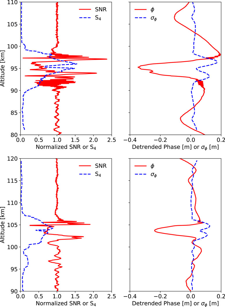
FIGURE 12. Two examples GNSS-RO measurements of sporadic-E layers: (top row) CDAAC descriptor atmPhs_C006.2014.024.22.34.G18_2013.3520_nc, (bottom row) atmPhs_C001.2014.179.18.34.G02_2014.2050_nc. Note the asymmetry in the signal amplitude (SNR) and detrended phase (ϕ) similar to the simulations in Figures 8, 9 after the K-H billows have formed.

Another natural extension of this research is to include the power law spectra derived from two-fluid simulations in large-scale multiple phase screen simulations such as Emmons et al. (2022). The layers produced here show PSDs that differ from the previously assumed Kolmogorov spectrum, which can help improve agreement with observations and ultimately improve E_s measurements from RO observations. Further, since this is a single case study, a series of simulations should be repeated using a variety of realistic initial conditions to statistically determine the PSD parameters and impact on GNSS signals.

5 Conclusion

This study showed the impacts of Kelvin-Helmholtz billow formation on GNSS radio occultation measurements of sporadic-E. K-H billows were simulated using a two-fluid model with a uniform sporadic-E layer as the initial condition. The time-varying ion density profiles were then used to create phase maps for a multiple phase screen model, which were used to simulate RO signals through the sporadic-E layer over time.

The resulting simulations showed a large variation in both the amplitude and phase profiles at the RO measurement plane as the K-H billows formed. Initially, before K-H billow formation, the thin, symmetric sporadic-E layer resulted in significant focusing of the GNSS-RO signal, producing large amplitude (S₄) and phase (σ_ϕ) scintillation. As the K-H billows formed and evolved, the sporadic-E layer became vertically thicker and less symmetric, effectively introducing imperfections to the sporadic-E lens. These imperfections and expansions ultimately reduce the severity of GNSS-RO signal focusing, which in turn reduces amplitude and phase scintillations. Further, the power spectra were shown to evolve over time with billow formation, decreasing in magnitude as small-scale structures began to develop.

The large variations in amplitude and phase over a relatively short during of 5 min indicate that a single E_s layer can produce a variety of RO observations depending on the turbulence/billow conditions, which could result in significant variations in sporadic-E parameter estimates derived from the RO observations. To truly understand RO observations of sporadic-E, we must understand the small-scale, turbulent, time dependent nature of sporadic-E, and this paper takes an important step towards modeling and including these effects.

While this study provides a single case study showing the proof of concept, a much larger set of simulations and observations is required to fully understand the spatial and temporal dynamics of sporadic-E. Extending the simulations to a wide variety of conditions would help to provide statistical significance to the results. Finally, obtaining a collection of GNSS-RO observations through K-H billows as measured by an ISR would provide crucial validation data for the models.

Data availability statement

The raw data supporting the conclusion of this article will be made available by the authors, without undue reservation.

Author contributions

AK: Data curation, Formal Analysis, Investigation, Methodology, Software, Writing–original draft, Writing–review and editing. DE: Conceptualization, Funding acquisition, Resources, Writing–original draft, Writing–review and editing.

Funding

The author(s) declare financial support was received for the research, authorship, and/or publication of this article. This research was funded by the Air Force Office of Scientific Research (AFOSR/RTB1).

Acknowledgments

We would like to thank the COSMIC Data Analysis and Archive Center (CDAAC) for the use of their data.

Conflict of interest

The authors declare that the research was conducted in the absence of any commercial or financial relationships that could be construed as a potential conflict of interest.

Publisher’s note

All claims expressed in this article are solely those of the authors and do not necessarily represent those of their affiliated organizations, or those of the publisher, the editors and the reviewers. Any product that may be evaluated in this article, or claim that may be made by its manufacturer, is not guaranteed or endorsed by the publisher.

References

Ansari, K., Panda, S. K., Kavutarapu, V., and Jamjareegulgarn, P. (2023). Towards mitigating the effect of plasma bubbles on GPS positioning accuracy through wavelet transformation over Southeast Asian region. Adv. Space Res. doi:10.1016/j.asr.2023.04.041

CrossRef Full Text | Google Scholar

Arras, C., and Wickert, J. (2018). Estimation of ionospheric sporadic E intensities from GPS radio occultation measurements. J. Atmos. Solar-Terrestrial Phys. 171, 60–63. doi:10.1016/j.jastp.2017.08.006

CrossRef Full Text | Google Scholar

Bernhardt, P. A. (2002). The modulation of sporadic-E layers by Kelvin–Helmholtz billows in the neutral atmosphere. J. Atmos. solar-terrestrial Phys. 64, 1487–1504. doi:10.1016/s1364-6826(02)00086-x

CrossRef Full Text | Google Scholar

Bilitza, D., Pezzopane, M., Truhlik, V., Altadill, D., Reinisch, B. W., and Pignalberi, A. (2022). The International Reference Ionosphere model: a review and description of an ionospheric benchmark. Rev. Geophys. 60, e2022RG000792. doi:10.1029/2022rg000792

CrossRef Full Text | Google Scholar

Bond, D., Wheatley, V., and Samtaney, R. (2016). “Plasma flow simulation using the two-fluid model,” in Proceedings of the 20th australasian fluid mechanics conference (Perth, Australia).

Google Scholar

Briggs, B., and Parkin, I. (1963). On the variation of radio star and satellite scintillations with zenith angle. J. Atmos. Terr. Phys. 25, 339–366. doi:10.1016/0021-9169(63)90150-8

CrossRef Full Text | Google Scholar

Chu, Y.-H., Wang, C., Wu, K., Chen, K., Tzeng, K., Su, C.-L., et al. (2014). Morphology of sporadic E layer retrieved from COSMIC GPS radio occultation measurements: wind shear theory examination. J. Geophys. Res. Space Phys. 119, 2117–2136. doi:10.1002/2013ja019437

CrossRef Full Text | Google Scholar

Emmert, J. T., Drob, D. P., Picone, J. M., Siskind, D. E., Jones, M., Mlynczak, M., et al. (2021). NRLMSIS 2.0: a whole-atmosphere empirical model of temperature and neutral species densities. Earth Space Sci. 8, e2020EA001321. doi:10.1029/2020ea001321

CrossRef Full Text | Google Scholar

Emmons, D. J., Wu, D. L., and Swarnalingam, N. (2022). A statistical analysis of sporadic-e characteristics associated with gnss radio occultation phase and amplitude scintillations. Atmosphere 13, 2098. doi:10.3390/atmos13122098

CrossRef Full Text | Google Scholar

Fabrizio, G. A. (2013). High frequency over-the-horizon radar: fundamental principles, signal processing, and practical applications. McGraw-Hill Education.

Google Scholar

Gooch, J. Y., Colman, J. J., Nava, O. A., and Emmons, D. J. (2020). Global ionosonde and GPS radio occultation sporadic-E intensity and height comparison. J. Atmos. Solar-Terrestrial Phys. 199, 105200. doi:10.1016/j.jastp.2020.105200

CrossRef Full Text | Google Scholar

Hakim, A., Loverich, J., and Shumlak, U. (2006). A high resolution wave propagation scheme for ideal two-fluid plasma equations. J. Comput. Phys. 219, 418–442. doi:10.1016/j.jcp.2006.03.036

CrossRef Full Text | Google Scholar

Haldoupis, C. (2011). A tutorial review on sporadic E layers. Aeronomy Earth’s Atmos. Ionos., 381–394. doi:10.1007/978-94-007-0326-1_29

CrossRef Full Text | Google Scholar

Hodos, T. J., Nava, O. A., Dao, E. V., and Emmons, D. J. (2022). Global sporadic-e occurrence rate climatology using gps radio occultation and ionosonde data. J. Geophys. Res. Space Phys. 127, e2022JA030795. doi:10.1029/2022ja030795

CrossRef Full Text | Google Scholar

Hysell, D., Nossa, E., Larsen, M., Munro, J., Smith, S., Sulzer, M., et al. (2012). Dynamic instability in the lower thermosphere inferred from irregular sporadic E layers. J. Geophys. Res. Space Phys. 117. doi:10.1029/2012ja017910

CrossRef Full Text | Google Scholar

Hysell, D., Nossa, E., Larsen, M., Munro, J., Sulzer, M., and González, S. (2009). Sporadic E layer observations over Arecibo using coherent and incoherent scatter radar: assessing dynamic stability in the lower thermosphere. J. Geophys. Res. Space Phys. 114. doi:10.1029/2009ja014403

CrossRef Full Text | Google Scholar

Hysell, D. L., Larsen, M., and Sulzer, M. (2016). Observational evidence for new instabilities in the midlatitude <i&amp;gt;E&amp;lt;/i&amp;gt; and <i&amp;gt;F&amp;lt;/i&amp;gt; region. Ann. Geophys. 34, 927–941. doi:10.5194/angeo-34-927-2016

CrossRef Full Text | Google Scholar

Jackson, J. D. (1999). Classical electrodynamics (American association of physics teachers).

Google Scholar

Knepp, D. L. (1983). Multiple phase-screen calculation of the temporal behavior of stochastic waves. Proc. IEEE 71, 722–737. doi:10.1109/proc.1983.12660

CrossRef Full Text | Google Scholar

Kyzyurov, Y. V. (2000). On the spectrum of mid-latitude sporadic-E irregularities. Ann. Geophys. 18, 1283–1292. doi:10.1007/s005850000259

CrossRef Full Text | Google Scholar

Levy, M., and Lerwitworapong, J. (2000). Issues facing TB control (3.1). Tuberculosis in prisons. Scott. Med. J. 45 (IET), 30–32; discussion 33. doi:10.1177/00369330000450S114

PubMed Abstract | CrossRef Full Text | Google Scholar

Maeda, J., and Heki, K. (2014). Two-dimensional observations of midlatitude sporadic E irregularities with a dense GPS array in Japan. Radio Sci. 49, 28–35. doi:10.1002/2013rs005295

CrossRef Full Text | Google Scholar

Maeda, J., and Heki, K. (2015). Morphology and dynamics of daytime mid-latitude sporadic-E patches revealed by GPS total electron content observations in Japan. Earth, Planets Space 67, 89–9. doi:10.1186/s40623-015-0257-4

CrossRef Full Text | Google Scholar

Neubeck, K. (1996). Using the combined resources of amateur radio observations and ionosonde data in the study of temperate zone sporadic-E. J. Atmos. Terr. Phys. 58, 1355–1365. doi:10.1016/0021-9169(95)00170-0

CrossRef Full Text | Google Scholar

Nishioka, M., Saito, A., and Tsugawa, T. (2008). Occurrence characteristics of plasma bubble derived from global ground-based GPS receiver networks. J. Geophys. Res. Space Phys. 113. doi:10.1029/2007ja012605

CrossRef Full Text | Google Scholar

Niu, J., Weng, L., Meng, X., and Fang, H. (2019). Morphology of ionospheric sporadic E layer intensity based on COSMIC occultation data in the midlatitude and low-latitude regions. J. Geophys. Res. Space Phys. 124, 4796–4808. doi:10.1029/2019ja026828

CrossRef Full Text | Google Scholar

Nygren, T., Jalonen, L., Oksman, J., and Turunen, T. (1984). The role of electric field and neutral wind direction in the formation of sporadic E-layers. J. Atmos. Terr. Phys. 46, 373–381. doi:10.1016/0021-9169(84)90122-3

CrossRef Full Text | Google Scholar

Panda, S. K., Moses, M., Ansari, K., and Walo, J. (2023). Ionospheric scintillation characteristics over Indian region from latitudinally-aligned geodetic GPS observations. Earth Sci. Inf. 16, 2675–2691. doi:10.1007/s12145-023-01070-z

CrossRef Full Text | Google Scholar

Rino, C. (2011). The theory of scintillation with applications in remote sensing. John Wiley and Sons.

Google Scholar

Savitzky, A., and Golay, M. J. (1964). Smoothing and differentiation of data by simplified least squares procedures. Anal. Chem. 36, 1627–1639. doi:10.1021/ac60214a047

CrossRef Full Text | Google Scholar

Schunk, R., and Nagy, A. (2009). Ionospheres: physics, plasma physics, and chemistry. The Edinburgh Building, Cambridge, United Kingdom: Cambridge University Press.

Google Scholar

Stambovsky, D. W., Colman, J. J., Nava, O. A., and Emmons, D. J. (2021). Simulation of GPS radio occultation signals through Sporadic-E using the multiple phase screen method. J. Atmos. Solar-Terrestrial Phys. 214, 105538. doi:10.1016/j.jastp.2021.105538

CrossRef Full Text | Google Scholar

Thébault, E., Finlay, C. C., Beggan, C. D., Alken, P., Aubert, J., Barrois, O., et al. (2015). International geomagnetic reference field: the 12th generation. Earth, Planets Space 67, 79–19. doi:10.1186/s40623-015-0228-9

CrossRef Full Text | Google Scholar

Whitehead, J. (1989). Recent work on mid-latitude and equatorial sporadic-E. J. Atmos. Terr. Phys. 51, 401–424. doi:10.1016/0021-9169(89)90122-0

CrossRef Full Text | Google Scholar

Wu, D. L., Ao, C. O., Hajj, G. A., de La Torre Juarez, M., and Mannucci, A. J. (2005). Sporadic E morphology from GPS-CHAMP radio occultation. J. Geophys. Res. Space Phys. 110. doi:10.1029/2004ja010701

CrossRef Full Text | Google Scholar

Wu, D. L., Emmons, D. J., and Swarnalingam, N. (2022). Global GNSS-RO electron density in the lower ionosphere. Remote Sens. 14, 1577. doi:10.3390/rs14071577

CrossRef Full Text | Google Scholar

Yu, B., Scott, C. J., Xue, X., Yue, X., and Dou, X. (2020). Derivation of global ionospheric Sporadic E critical frequency (f_oEs) data from the amplitude variations in GPS/GNSS radio occultations. R. Soc. open Sci. 7, 200320. doi:10.1098/rsos.200320

PubMed Abstract | CrossRef Full Text | Google Scholar

Yu, B., Xue, X., Scott, C. J., Yue, X., and Dou, X. (2022). An empirical model of the ionospheric sporadic E layer based on GNSS radio occultation data. Space weather. 20, e2022SW003113. doi:10.1029/2022sw003113

CrossRef Full Text | Google Scholar

Yue, X., Schreiner, W. S., Pedatella, N. M., and Kuo, Y.-H. (2016). Characterizing GPS radio occultation loss of lock due to ionospheric weather. Space weather. 14, 285–299. doi:10.1002/2015sw001340

CrossRef Full Text | Google Scholar

Zeng, Z., and Sokolovskiy, S. (2010). Effect of sporadic E clouds on GPS radio occultation signals. Geophys. Res. Lett. 37. doi:10.1029/2010GL044561

CrossRef Full Text | Google Scholar