LAPS: An MPI-parallelized 3D pseudo-spectral Hall-MHD simulation code incorporating the expanding box model

1 Introduction

Plasma physics, including space plasmas, encompasses complex nonlinear and multi-scale phenomena that often require the use of direct numerical simulations. Such is the case of turbulence, reconnection and nonlinear wave-particle interactions, to give a few examples. Thanks to the ever increasing numerical capabilities of high-performance computing, direct numerical simulations have proved an indispensable tool to further understanding of many plasma phenomena occurring in space, by providing much needed support to the interpretation of spacecraft observations (e.g., Jia et al., 2012; Shi et al., 2022; Dorfman et al., 2023).

Space and astrophysical plasmas mainly consist of highly-ionized plasmas, thus, different numerical models are employed depending on the specific phenomenon or temporal, as well as spatial, scale of the system that is being studied. These numerical models include Vlasov (see Palmroth et al., 2018, and references therein), Particle-in-Cell (PIC) (e.g., Markidis and Lapenta, 2010), hybrid PIC (e.g., Lin et al., 2014), and magnetohydrodynamic (MHD) (e.g., Tóth et al., 2012) models. In particular, the MHD model has proved successful to describe a variety of solar and heliophysics phenomena, and there has been a significant effort in the heliophysics community to develop efficient and scalable MHD codes (e.g., Mignone et al., 2007; van der Holst et al., 2014; Shoda et al., 2019; Réville et al., 2020). Although the most frequently used spatial-discretization method in MHD simulations is the finite-volume method with selected Riemann solvers (e.g., Eymard et al., 2000; Miyoshi and Kusano, 2005) because of its ability to deal with unstructured mesh and to capture shocks, the pseudo-spectral method based on the Fourier transform is very useful for problems that can be described in a domain with periodic boundary conditions. The pseudo-spectral method has the advantage of very high efficiency and can accurately calculate the spatial derivatives up to grid scale. Hence, it is especially suitable for simulating systems that require accurate resolution of small scale dynamics, such as turbulence.

Here, we present an open-source three-dimensional (3D) pseudo-spectral MHD code LAPS (UCLA-Pseudo-Spectral) based on Fast-Fourier-transform (FFT). The code is written in FORTRAN. It utilizes the external package FFTW (Frigo and Johnson, 2005) for FFT, and is parallelized using Message-Passing-Interface (MPI). We adopt a “pencil” parallelization strategy so that the code can achieve very high scalability. The code is equipped with an Hall-MHD module and an incompressible version has also been developed to investigate the effects of ion kinetic physics and compressibility on various MHD processes. In addition, the expanding-box-model (EBM) (Grappin and Velli, 1996; Tenerani and Velli, 2017) has been implemented to simulate the dynamic processes happening in the expanding solar wind, such as solar wind turbulence.

The paper is organized as follows. In Section 2, we describe in detail the numerical methods of the code, including the model equations, time advancement method, and numerical filters, etc. In Section 3, we discuss our parallelization strategy and present the scalability tests of the code. In Section 4, we show four test cases, including 1) incompressible Hall-MHD waves, 2) incompressible tearing mode instability, 3) the Orszag-Tang vortex test, and 4) parametric decay instability. In Section 5, we summarize this paper.

2 Code description

2.1 Compressible Hall-MHD equation set

The base version of the code integrates the compressible Hall-MHD equation set written in the following normalized form:

$\frac{\partial \rho }{\partial t}=-\nabla \cdot \left(\rho \mathit{U}\right)(\mathrm{1a})$

$\frac{\partial \left(\rho \mathit{U}\right)}{\partial t}=-\nabla \cdot \left[\rho \mathit{U}\mathit{U}+\left(P+\frac{1}{2}{B}^2\right)\mathit{I}-\mathit{B}\mathit{B}\right]+\nu {\nabla }^2\left(\rho \mathit{U}\right)(\mathrm{1b})$

$\frac{\partial \mathit{B}}{\partial t}=-\nabla \times \mathit{E}+\eta {\nabla }^2\mathit{B}(\mathrm{1c})$

$\frac{\partial e}{\partial t}=-\nabla \cdot \left[\left(e+P+\frac{1}{2}{B}^2\right)\mathit{U}-\left(\mathit{U}\cdot \mathit{B}\right)\mathit{B}\right](\mathrm{1d})$

where ρ, U, P, and B are density, velocity, thermal pressure, and magnetic field respectively,

$e=\frac{P}{\gamma -1}+\frac{1}{2}\rho U^2+\frac{1}{2}{B}^2$

is the total energy density with γ being the adiabatic index typically set as γ = 5/3,

$\mathit{E}=-\mathit{U}\times \mathit{B}+\frac{d_i}{\rho }\mathit{J}\times \mathit{B}$

is the electric field with J = ∇ ×B being the electric current density and d_i being the normalized ion inertial length. ν and η are explicit viscosity and resistivity. In Eq. 1, all quantities are normalized. One can freely select units for length L, density $\bar{\rho }$, and magnetic field strength $\bar{B}$. From these units, one can further derive unit of speed $\bar{U}=\bar{B}/\sqrt{{\mu }_0\bar{\rho }}$, unit of time $\tau =L/\bar{U}$, and unit of pressure $\bar{P}={\bar{B}}^2/{\mu }_0$. In addition, the viscosity ν and resistivity η are essentially the inverses of the dimensionless Reynolds number $R_e=L\bar{U}/\tilde{\nu }$ and Lundquist number $S=L\bar{U}/\tilde{\eta }$ where $\tilde{\nu }$ and $\tilde{\eta }$ are viscosity and resistivity in physical units.

We note that the viscous term in Eq. 1b is different from the commonly-used form νρ∇²U. In this way, we are able to calculate the viscous term in Fourier space directly because ρU, instead of U, is the quantity being evolved. The exact form of this term is not important because typically the viscosity is used only for the purpose of numerical stability. Compared with viscosity, the resistivity not only serves as a numerical stabilizer, but also is crucial in the triggering of magnetic reconnection (e.g., the test case of tearing instability shown in Section 4.2). The values of ν and η depend on the specific problems being studied. Simulations without strong nonlinear processes are typically stable even without ν and η. In simulations with strong nonlinearity, such as simulations of turbulence, the diffusion should be strong enough to dissipate the cascaded turbulence energy. In this case, the values of ν and η should be larger than N^−4/3 with N being the number of grid points.

We would like to emphasize that, given the form of Eq. 1d and the total energy contained in the simulation domain $\mathcal{E}={\int }_{V}e$ is exactly conserved, just like the total mass M = ∫_Vρ, i.e., $d\mathcal{E}/dt=dM/dt=0$. Even if the viscosity and resistivity are finite, the loss of kinetic and magnetic energies due to diffusion automatically add to the internal energy of the plasma, conserving the total energy. This will be verified in the Orszag-Tang vortex test (Section 4.3).

2.2 Time advancement

We use the explicit Van der Houwen’s/Wray third-order Runge-Kutta method (Van der Houwen, 1972; Wray, 1990) to integrate Eq. 1. The coefficients of this method are summarized in the following table

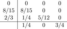
This method has the advantage of low-storage request. For an equation (set) of the form

$\frac{df}{dt}=F\left(f\right),$

each time step (from n to n + 1) consists of three sub-steps.

$f^{n+\frac{1}{3}}=f^n+F\left(f^n\right)\times \frac{8}{15}\mathrm{\Delta }t(\mathrm{3a})$

$f^{n+\frac{2}{3}}=f^{n+\frac{1}{3}}-F\left(f^n\right)\times \frac{17}{60}\mathrm{\Delta }t+F\left(f^{n+\frac{1}{3}}\right)\times \frac{5}{12}\mathrm{\Delta }t(\mathrm{3b})$

$f^{n+1}=f^{n+\frac{2}{3}}-F\left(f^{n+\frac{1}{3}}\right)\times \frac{5}{12}\mathrm{\Delta }t+F\left(f^{n+\frac{2}{3}}\right)\times \frac{3}{4}\mathrm{\Delta }t(\mathrm{3c})$

where Δt is the size of the time step. Eq. 3 shows that only one additional copy of F(f) from the previous sub-step is needed. This feature can be very helpful in the case that the available memory is limited. We note that, a third-order Runge-Kutta method in general introduces stronger numerical dissipation than higher-order methods such as the fourth-order Dormand–Prince method (Dormand and Prince, 1980). Nonetheless, it reduces the computational time significantly. We will implement more time-integral methods in the future.

The size of the time step Δt is determined by the Courant–Friedrichs–Lewy (CFL) condition (De Moura and Kubrusly, 2013)

$\mathrm{\Delta }t\le C_t\times \frac{\mathrm{\Delta }x}{\mathrm{m}\mathrm{a}\mathrm{x}\left(U_w\right)}(4)$

where C_t is a constant typically between 0.1 and 0.5 and is adjustable in the code, Δx is the grid spacing, e.g., along x direction, and U_w refers to the speed of the fastest-propagating wave mode along that direction. As a hyperbolic system, the ideal MHD equation set allows seven wave modes, namely, the entropy mode, two Alfvén modes, two slow magnetosonic modes, and two slow magnetosonic modes. The propagation speeds of the seven modes along a given direction, e.g., x, are

$U_x,U_x\pm U_{A,x},U_x\pm U_{s,x},U_x\pm U_{f,x}(5)$

respectively. Here, U_x is the flow speed projected along x-direction, $U_{A,x}=B_x/\sqrt{\rho }$ is the projected Alfvén speed, U_(s,f),x are the projected slow and fast magnetosonic speeds

$U_{\left(s,f\right),x}=\frac{1}{\sqrt{2}}{\left[U_m^2\mp U_{n,x}^2\right]}^{\frac{1}{2}}$

where

$U_m^2=U_s^2+U_A^2,U_{n,x}^2={\left[U_m^4-4U_s^2{U}_{A,x}^2\right]}^{\frac{1}{2}},$

$U_s=\sqrt{\gamma P/\rho }$ is the sound speed, and $U_A=\left|B\right|/\sqrt{\rho }$ is the amplitude of Alfvén speed. For the Hall-MHD system, the speed of the dispersive whistler wave, which is typically the fastest-propagating wave mode, needs to be included, and we use $U_{\mathit{Hall}}\sim \frac{d_{i}B}{\rho \mathrm{\Delta }x}$ to approximate this speed.

In the code, we first calculate Δt_x, Δt_y, Δt_z, i.e., time step sizes determined along different directions, at each grid point, and adopt the smallest one among the three values. Then we scan all the grid points to determine the smallest Δt in the system. For the incompressible version of the code which will be discussed in Section 2.3, only the speeds of Alfvén and whistler waves need to be considered in the estimate of Δt due to the absence of compressive fluctuations. In expanding-box simulations which will be discussed in Section 2.5, the transverse grid scales increase with time and become much larger than the radial grid scale, which remains constant. In this case, the radial grid scale is the most important in the estimate of Δt. We note that, with finite ν or η, one needs to take the diffusion rate into account in the estimate of Δt. Nonetheless, as the diffusion time scale, τ_d ∼Δx²/ν or τ_d ∼Δx²/η is typically much larger than the wave propagation time scale, we neglect the diffusion effect in the calculation of Δt. Last, we note that Δt is adaptively determined during the simulation, i.e., the code re-evaluates Δt after each time step. This is necessary in long-duration simulations where the fields change significantly from the initial status.

Figure 1 shows the flow chart of one sub time step for the compressible code. In this chart, boxes filled with blue color correspond to operations in Fourier space, and boxes without filling correspond to operations in configuration space. We call the variables $\left(\rho ,\rho \mathit{U},\mathit{B},e\right)$ “fields”, which are evolved in time. At each sub time step, we first calculate the “fluxes”

$\rho \mathit{U},\rho \mathit{U}\mathit{U}+\left(P+\frac{1}{2}{B}^2\right)\mathit{I}-\mathit{B}\mathit{B},\mathit{E},\left(e+P+\frac{1}{2}{B}^2\right)\mathit{U}-\left(\mathit{U}\cdot \mathit{B}\right)\mathit{B}$

in configuration space and transform these fluxes to Fourier space. Note that, for the induction equation, we are using the electric field E instead of a flux. However, for convenience, we still call it a “flux”. Then, we integrate the equation set in Fourier space after calculating the r.h.s of Eq. 1, which involves inner product and cross product between the wave vector k and the fluxes as well as multiplication of −k² and the fields. In particular, the magnetic field is advanced by

$\frac{\partial {\mathit{B}}_{\mathit{k}}}{\partial t}=-i\mathit{k}\times {\mathit{E}}_{\mathit{k}}-\eta k^2{\mathit{B}}_{\mathit{k}},(6)$

which automatically preserves ∇ ⋅B = 0 to round-off error if the initial magnetic field has zero divergence. Therefore, in LAPS, no ∇ ⋅B cleaning is required. After the time integral, we apply a numerical filter to all the fields, which will be described in detail in Section 2.4. Lastly, we apply the inverse Fourier transform to ρ_k, ${\left(\rho \mathit{U}\right)}_{\mathit{k}}$, B_k, e_k, and J_k = ik ×B_k to derive these quantities in configuration space.

Figure 1

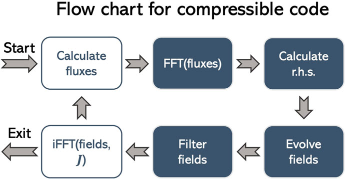
Figure 1. Flow chart of each sub time step for the compressible version of the code. Boxes filled with blue color correspond to operations in Fourier space, and boxes without filling correspond to operations in configuration space.

2.3 Incompressible version

As the level of compressible fluctuations in the solar wind is typically small (Shi et al., 2021), incompressibility is often assumed to simplify the theoretical models or reduce the cost of simulations in the study of solar wind turbulence (e.g., Perez and Chandran, 2013). However, recent numerical investigations suggest that compressive processes may play a significant role in the dynamics of solar wind, such as the development of turbulence (Shoda et al., 2019; Tenerani et al., 2020). To explore how the assumption of incompressibility affects different processes, such as the turbulence evolution, we have developed an incompressible version of the code.

In the incompressible code, we impose a uniform density ρ and use the thermal pressure P to enforce the ∇ ⋅U = 0 condition. Thus, only U and B are evolved in time. The thermal pressure must satisfy

${\nabla }^{2}P=\nabla \cdot \left[-\rho \mathit{U}\cdot \nabla \mathit{U}+\mathit{J}\times \mathit{B}\right](7)$

so that ${\partial }_t\left(\nabla \cdot \mathit{U}\right)\equiv 0$. The flow chart of the incompressible code is shown in Figure 2. At each sub time step, we first calculate J_k and ikU_k in Fourier space and inverse transform them to get J and ∇U in configuration space. Next, we calculate the “flux” for pressure, i.e., the term in the bracket on the r.h.s of Eq. 7, and Fourier transform this term. This leads to the solution of pressure in Fourier space: −k²P_k = ik ⋅F_P,k where F_P,k is the Fourier mode of −ρU ⋅∇U + J ×B. Note that for thermal pressure, the k = 0 mode is negligible. In practice, it is unnecessary to solve P_k because we are only interested in ${\partial }_t{\left(\rho \mathit{U}\right)}_{\mathit{k}}$, which is

$\frac{\partial {\left(\rho \mathit{U}\right)}_{\mathit{k}}}{\partial t}={\mathit{F}}_{P,\mathit{k}}-\mathit{k}\frac{\mathit{k}\cdot {\mathit{F}}_{P,\mathit{k}}}{k^2}-k^2\nu {\left(\rho \mathit{U}\right)}_{\mathit{k}}(8)$

For the magnetic field, we simply calculate electric field in the configuration space, Fourier transform it, and get the r.h.s of Eq. 6. Finally, we evolve U_k and B_k, filter the evolved fields, and inverse transform the fields.

Figure 2

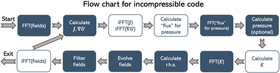
Figure 2. Flow chart of each sub time step for the incompressible version of the code. Boxes filled with blue color correspond to operations in Fourier space, and boxes without filling correspond to operations in configuration space.

2.4 Filtering and de-aliasing

Because the evolved equation set contains nonlinear terms, numerical filtering or de-aliasing is necessary to remove the high-wavenumber fluctuations. In LAPS, a zero-padding de-aliasing is implemented, which removes all the fluctuations on wave modes M ≥ 1/3 after each sub time step. Here M is the normalized wave mode

$M=\sqrt{{\left(\frac{m_x}{N_x}\right)}^2+{\left(\frac{m_y}{N_y}\right)}^2+{\left(\frac{m_z}{N_z}\right)}^2}$

where (N_x, N_y, N_z) are number of grid points along each direction, $-\frac{N_x}{2}\le m_x\le \frac{N_x}{2}$ is the wave mode in x and similarly form_y and m_z.

In practice, we find that a numerical filter, which is a smooth function of k, is very efficient in removing the high wavenumber fluctuations while maintaining stability of the simulation without too strong dissipation of the fields. The function form of the filter is inspired by the filter frequently implemented in compact finite difference schemes (Lele, 1992):

$T\left(k\right)=\frac{a+b\cos \left(w\right)+c\cos \left(2w\right)}{1+2\lambda \cos \left(w\right)}(9)$

where w = 2πkΔ is the normalized wave number along a specific direction and takes values between −π and π. Δ is the grid spacing. a = (5 + 6α)/8, b = (1 + 2α)/2, c = −(1 − 2α)/8 are three parameters dependent on the free parameter α, usually between 0.45 and 0.5. The smaller α is, the stronger the filter is. Especially, when α = 0.5, there is no filtering. For multi-dimensional case, the filter is defined as T(k) = T(k_x) × T(k_y) × T(k_z). After each sub time step or time step, we apply the filter by multiplying the evolved fields by T(k). We note that, applying the filter does not break the ∇ ⋅B = 0 condition. The reason is that all of the three components of B_k are multiplied by the same function T(k). Therefore, the filtered magnetic field is simply ${\tilde{\mathit{B}}}_{\mathit{k}}=T(\mathit{k}){\mathit{B}}_{\mathit{k}}$, i.e., $\mathit{k}\cdot {\tilde{\mathit{B}}}_{\mathit{k}}=T(\mathit{k})\times (\mathit{k}\cdot {\mathit{B}}_{\mathit{k}})$ = 0.

2.5 Expanding-box-model

In simulations of dynamic processes happening in the solar wind, the large-scale spherical expansion of solar wind is non-negligible because it leads to inhomogeneity of the background fields and anisotropic evolution of different components of velocity and magnetic field. To incorporate the expansion effect into simulations of local processes, expanding-box-model (EBM) has been developed and implemented in MHD (Grappin and Velli, 1996), hybrid (Liewer et al., 2001; Hellinger et al., 2003), and PIC (Innocenti et al., 2019) simulations. In the classic EBM, a plasma parcel that moves along the radial direction with a constant speed U₀ is simulated. EBM for MHD with a time-dependent U₀, i.e., “accelerating” EBM, was developed by Tenerani and Velli (2017), but so far LAPS only allows a constant U₀ and will be equipped with the accelerating EBM in the future. The plasma parcel expands in the transverse direction with an expansion time scale τ = R(t)/U₀ where R(t) = R₀ + U₀t is the radial distance to the origin, e.g., the center of the Sun, and R₀ is the initial radial location of the plasma parcel. A more detailed explanation of the EBM can be found in (Grappin and Velli, 1996; Tenerani and Velli, 2017; Shi et al., 2020b) and will not be repeated here. Assuming that x is aligned with the radial direction, a pseudo-Galilean transform with respect to the average radial speed $U_0{\widehat{e}}_r$ leads to additional “expansion” terms

$\begin{array}{cc}\hfill & S_{\rho }=-\frac{2}{\tau }\rho ,{\mathit{S}}_{\mathit{U}}=-\frac{1}{\tau }\left(\begin{array}{ccc}\hfill 2\hfill & \hfill 0\hfill & \hfill 0\hfill \\ \hfill 0\hfill & \hfill 3\hfill & \hfill 0\hfill \\ \hfill 0\hfill & \hfill 0\hfill & \hfill 3\hfill \end{array}\right)\rho \mathit{U},{\mathit{S}}_{\mathit{B}}=-\frac{1}{\tau }\left(\begin{array}{ccc}\hfill 2\hfill & \hfill 0\hfill & \hfill 0\hfill \\ \hfill 0\hfill & \hfill 1\hfill & \hfill 0\hfill \\ \hfill 0\hfill & \hfill 0\hfill & \hfill 1\hfill \end{array}\right)\mathit{B},\hfill \\ \hfill & S_e=-\frac{1}{\tau }\left[\frac{2\gamma }{\gamma -1}P+\rho \left(U_x^2+2U_y^2+{2U}_z^2\right)+\left(2B_x^2+B_y^2+B_z^2\right)\right],\hfill \end{array}(10)$

that need to be added to the r.h.s of Eq. 1. Here, S_ρ, S_U, and S_B can be calculated directly in Fourier space while S_e must be calculated in the configuration space first and then Fourier transformed. We note that, with EBM, the grid spacing along the transverse directions (y and z) increases with time. Consequently, the transverse wavenumbers must be updated after every time step:

$k_y=k_{y,0}\times \frac{R_0}{R\left(t\right)},k_z=k_{z,0}\times \frac{R_0}{R\left(t\right)}.$

A “corotation” module that allows a non-radial x-axis is implemented so that the code is able to simulate the corotating-interaction-regions. The technical details of this module are documented in (Shi et al., 2020b).

One important question is whether the expansion term S_B preserves the ∇ ⋅B = 0 condition. To answer this question, let us write the normalized EBM coordinates (here we neglect z-direction which is exactly the same with y-direction) as $(\tilde{x},\tilde{y})$ such that

$\tilde{x}=x-R\left(t\right),\tilde{y}=\frac{R_0}{R\left(t\right)}y.(11)$

where (x, y) are coordinates of the Sun-centered stationary frame. This coordinate transform leads to: ${\partial }_x={\partial }_{\tilde{x}}$, ${\partial }_y=R_0/R\times {\partial }_{\tilde{y}}$. Then, we can calculate the time-derivative of ∇ ⋅B introduced by the expansion term:

$\begin{array}{cc}\hfill \frac{\partial }{\partial t}{\left(\nabla \cdot \mathit{B}\right)}_{\mathit{exp}}& =\frac{\partial }{\partial t}\left(\frac{\partial B_x}{\partial \tilde{x}}+\frac{R_0}{R}\frac{\partial B_y}{\partial \tilde{y}}\right)\hfill \\ \hfill & =\frac{\partial }{\partial \tilde{x}}\left(\frac{\partial B_x}{\partial t}\right)+\frac{R_0}{R}\frac{\partial }{\partial \tilde{y}}\left(\frac{\partial B_y}{\partial t}\right)-\frac{U{R}_0}{R^2}\frac{\partial B_y}{\partial \tilde{y}}\hfill \\ \hfill & =\frac{\partial }{\partial \tilde{x}}\left(-\frac{2B_x}{\tau }\right)+\frac{R_0}{R}\frac{\partial }{\partial \tilde{y}}\left(-\frac{B_y}{\tau }\right)-\frac{R_0}{R}\frac{1}{\tau }\frac{\partial B_y}{\partial \tilde{y}}\hfill \\ \hfill & =-\frac{2}{\tau }\left(\frac{\partial B_x}{\partial \tilde{x}}+\frac{R_0}{R}\frac{\partial B_y}{\partial \tilde{y}}\right)\hfill \\ \hfill & =-\frac{2}{\tau }\left(\nabla \cdot \mathit{B}\right)\hfill \end{array}$

Thus, the expansion term tends to decrease ∇ ⋅B. If ∇ ⋅B = 0 initially, the expansion term will not generate any net ∇ ⋅B.

As a final remark, so far the EBM is only implemented to the compressible version of the code, because it is a nontrivial task to make the EBM compatible with the assumption of incompressibility. One can show that the expansion tends to break the $\nabla \cdot \left(\rho \mathit{U}\right)=0$ condition because it leads to a faster decay of ${\partial }_y\left(\rho U_y\right)$ and ${\partial }_z\left(\rho U_z\right)$ than ${\partial }_x\left(\rho U_x\right)$ (Dong et al., 2014). Therefore, more works need to be done to properly implement EBM to the incompressible code.

3 Parallelization

Parallelization of pseudo-spectral codes, especially in 3D, is complex, because a large amount of communication between different processes is needed due to the non-locality of the pseudo-spectral method (Reuter et al., 2008).

To complete a 3D Fourier transform, an array needs to be transposed once or twice, depending on the parallelization strategy adopted. During one transpose operation, each process needs to send (nearly) the whole chunk of data it possesses to other processes and receive data of the similar volume. One choice of parallelization is to decompose the domain into “slabs”, i.e., to parallelize along one dimension such that each process handles a sub-layer of the domain (e.g., GHOST Mininni et al., 2011). This method has the advantage of less data transfer between processes because only one transpose operation is needed for 3D Fourier transform, but the computational workload of each process is heavy. In LAPS, we adopt another parallelization strategy and divide the simulation domain into “pencils” instead of slabs, i.e., we parallelize the domain along two dimensions, as illustrated by Figure 3. An array defined in the configuration space is parallelized along y and z directions. To transform the array to Fourier space, we apply Fourier transform along x direction first. Then the array is transposed in x-y plane so that y becomes the undivided dimension and Fourier transformed is applied along y direction. Last, we transpose the array in y-z plane and apply Fourier transform in z direction. Consequently, the array in Fourier space is parallelized in x (k_x) and y (k_y) directions. The inverse Fourier transform is conducted in the inverse order, i.e., starting from z-axis, then y-axis, and finally x-axis. This pencil-parallelization strategy requires more data transfer between different processes, but the computational workload of each process is lighter than slab-parallelization. Similar parallelization strategy is implemented in the external package P3DFFT for FFT of 3D arrays (Pekurovsky, 2012; Kawazura, 2022) as well as high-order finite-difference MHD code The Pencil Code (Brandenburg et al., 2021). We note that, the pencil-parallelization strategy is more suitable for clusters with large numbers of CPU cores, because much more sub-tasks are created compared with the slab-parallelization strategy. The slab-parallelization strategy, on the contrary, is expected to be very useful in a system with limited cores, e.g., multiple GPUs. Therefore, a promising future direction is to develop a GPU-accelerated version of the code with slab-parallelization strategy.

Figure 3

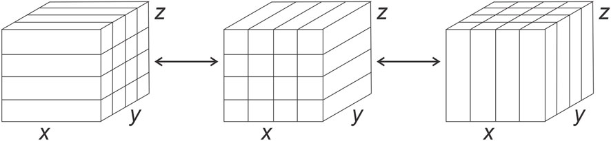
Figure 3. Layout of the data parallelized using “pencils”. A 3D array in configuration space is parallelized along y and z (left). During 3D Fourier transform, the array is first transposed in x − y plane (middle) and then transposed in y − z plane (right). Hence, the array in wave-vector space is parallelized along x and y.

To test the scalability of the code, we conducted two sets of strong scaling tests, i.e., the problem size is constant while the number of processors varies in each test, on UCAR/DERECHO cluster². The DERECHO cluster² contains 2488 CPU computation nodes, with 128 cores and 256 GB memory per node. The inter-node data transfer rate is approximately 200 GB/sec. The test results are shown in Table 1 and Figure 4. In Table 1, the top and bottom two rows are test runs with 512³ grid and 1,024³ grid respectively, and different columns are different numbers of processors used. We quantify the speed of the simulations by iterations per second. In addition, we quantify the speedup by normalizing the simulation speeds with different numbers of processors to the speed of the run with the least number of processors. Note that, for the test with a 1,024³ grid, we do not conduct runs with 128 and 256 processors due to the limit of memory of the cluster. Results listed in Table 1 are plotted in Figure 4, whose left panel shows the simulation speed as a function of number of processors and right panel shows the speedup as a function of the number of processors normalized to the least number of processors used in each test. The orange curves represent runs with 512³ grid, and the blue curves represent runs with 1,024³ grid. The blue curve in the left panel is multiplied by 8 for better visualization. As a reference, the black dashed lines show y ∝ x (left) and y = x (right), i.e., the ideal case when the speed is a linear function of the number of processors. The Pearson correlation coefficients for the orange and blue curves are 0.9975 and 0.9998 respectively (note that curves of the same color in the two panels have exactly the same shape and hence the same Pearson correlation coefficient). Thus, the speed of simulation is almost a linear function of the number of processors in both the two tests, indicating a very high scalability of the code.

Figure 4

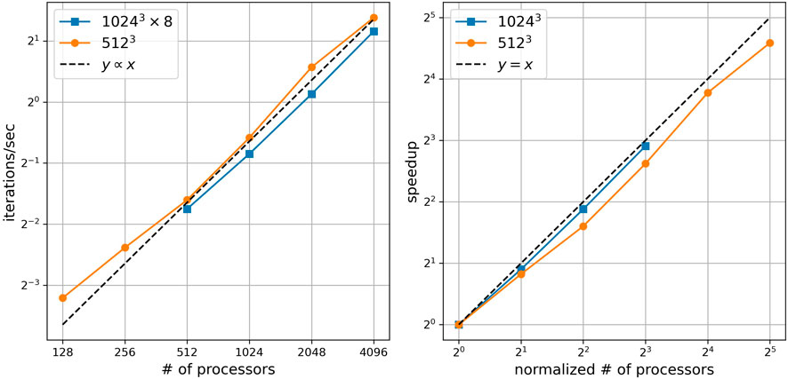
Figure 4. Visualization of the strong scaling test results displayed in Table 1. Left panel shows the simulation speed (iterations per second) as a function of number of processors. Right panel shows the speedup as a function of the number of processors normalized to the least number of processors used in each test. Blue curves are test runs with 1,024³ grid (Pearson correlation coefficient 0.9998) and orange curves are test runs with 512³ grid (Pearson correlation coefficient 0.9975). For better visualization, we have multiplied the speed of the 1,024³ runs by a factor of 8 in the left panel. The black dashed lines show the ideal case where the simulation speed is a linear function of the number of processors.

Table 1

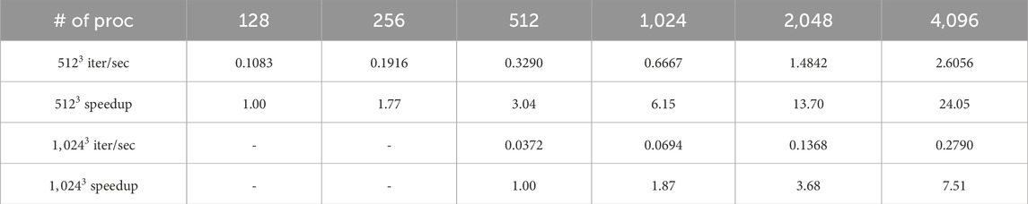
Table 1. Result of the two strong scaling tests of LAPS conducted on UCAR/DERECHO. Different columns correspond to different numbers of processors. For each test, we list the simulation speed quantified by iterations per second on the top and the speedup with respect to the run with the least number of processors on the bottom.

4 Test cases

To verify that LAPS works properly, we conducted four (sets of) test runs based on four benchmark physics problems. The results are presented below.

4.1 Incompressible Hall-MHD waves

The incompressible Hall-MHD system with a uniform background magnetic field has two eigen-modes whose dispersion relation is written as

$\omega =\frac{\sqrt{{\left(k{d}_i\right)}^2+4}\pm k{d}_i}{2}\left(\mathit{k}\cdot {\mathit{V}}_{\mathit{A}}\right).(12)$

Here ω is frequency, k is wave-vector, d_i is the ion inertial length, and ${\mathit{V}}_{\mathit{A}}={\mathit{B}}_{\mathbf{0}}/\sqrt{4\pi \rho }$ is the background magnetic field in Alfvén speed unit and ρ is the plasma density. “+” corresponds to the right-hand polarized whistler mode wave and “−” corresponds to the left-hand polarized ion cyclotron wave.

To verify the Hall-MHD module, we carry out a 1D simulation using the incompressible Hall-MHD code. De-aliasing instead of numerical filtering is activated. No viscosity or resistivity is implemented. The domain size is L_x = 8 and the number of grid is N_x = 1,024. The ion inertial length is d_i = 0.1. We initialize the simulation with a uniform density ρ = 1 and a uniform background field $\mathit{B}=1{\widehat{e}}_x$. The time step size is evaluated with C_t = 0.2 and the resultant Δt is roughly 1.2 × 10⁻⁴. Random fluctuations in B_z are added on wavenumbers k ∈ (0, 8]. We apply Fourier transform in x and in time during t ∈ [0.5, 2.5] to acquire the power spectrum density ${\left|B_z\left(k,\omega \right)\right|}^2$, which is shown in Figure 5. The two dashed white lines are the analytic dispersion relation given by Eq. 12. We can see that the simulation result is exactly consistent with the linear theory.

Figure 5

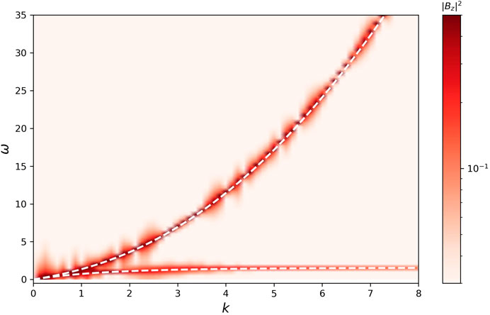
Figure 5. Dispersion relation ω(k) in a 1D incompressible Hall-MHD simulation with d_i =0.1. The plot is colorcoded with ${\left|B_z\left(k,\omega \right)\right|}^2$. The two white dashed lines are the two analytic solutions (Eq. 12).

4.2 Incompressible tearing mode instability

It is well known that a resistive current sheet is susceptible to the tearing mode instability (Furth et al., 1963), the growth of which can break an elongated current sheet into a chain of plasmoids rapidly. The theory of tearing instability in incompressible MHD was well established, and its growth rate can be calculated in a semi-analytic way (Pucci and Velli, 2013; Shi et al., 2020a; Shi, 2022). Thus, incompressible tearing instability is a very good benchmark for resistive-MHD code.

We conduct a 2D incompressible simulation, initialized with a Harris-type current sheet:

$\mathit{B}\left(x,y\right)=B_0\tanh \left(\frac{y-y_0}{a}\right){\widehat{e}}_x.(13)$

The density is uniform: ρ = 1, and the thermal pressure is used to maintain a uniform total pressure

$P\left(x,y\right)+\frac{1}{2}{B}^2\left(x,y\right)=P^T=2.(14)$

Note that because periodic boundary condition is enforced in the spectral code, we actually set up a double Harris current sheet, while the analysis only focuses on the lower current sheet. The size of the simulation domain is L_x = 128a and L_y = 60a with a = 1, and the number of grid is N_x = 256 and N_y = 1,024. De-aliasing is turned on without numerical filtering. The resistivity is η = 10^–3, corresponding to a Lundquist number S = 10³, and no viscosity is added. We select C_t = 0.5 and consequently the size of time step is Δt ≈ 0.25. We add fluctuations in magnetic field at the center of the current sheets, as shown in the top panel of Figure 6, which is color-coded with B_y. The middle and bottom panels show snapshots at t = 400 and t = 1,100 respectively. We can see the formation and nonlinear evolution of plasmoids due to the tearing instability.

Figure 6

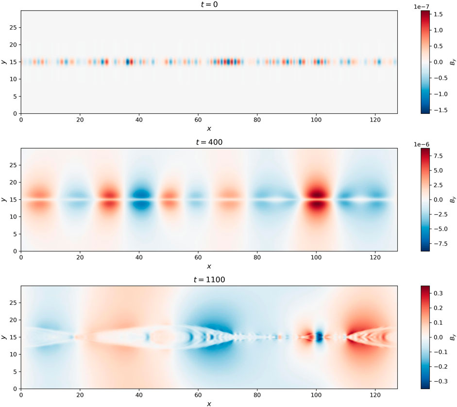
Figure 6. Evolution of B_y at t = 0 (top), t = 400 (middle), and t = 1,100 (bottom) in the 2D incompressible simulation of a resistive current sheet.

To quantify the linear growth rate of tearing instability, we apply Fourier transform to B_y along the central line of the current sheet y = y₀. Panel a) of Figure 7 shows the time evolution of the amplitudes of different Fourier modes. From purple to yellow, different lines correspond to wavelengths λ ∈ [128a, 8a]. Clearly there is a linear-growing phase in all the modes. We apply a linear fit between t = 200 and t = 400 (marked by the yellow shade) and acquire the growth rates for different modes. On Panel b), we show the fitted growth rate as a function of wavenumber in blue dots. The orange curve is the exact solution of the dispersion relation solved from the eigenvalue problem of incompressible tearing instability. More specifically, we solve the following boundary-value-problem.

$\gamma \left(u_y^{\prime \prime }-k^2{u}_y\right)=ik\left[B_x\left(b_y^{\prime \prime }-k^2{b}_y\right)-B_x^{\prime \prime }{b}_y\right](\mathrm{15a})$

$\gamma b_y=ik{B}_x{u}_y+\eta \left(b_y^{\prime \prime }-k^2{b}_y\right)(\mathrm{15b})$

Figure 7

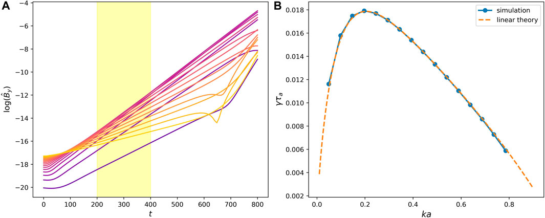
Figure 7. (A) Time evolution of the amplitudes of Fourier modes ${\widehat{B}}_y(k_x,y=y_0)$ calculated at the center of the current sheet. From purple to yellow lines are wavelengths λ ∈ [128a, 8a]. The yellow shade marks the time interval for calculation of growth rates. (B) Blue dots are the calculated growth rate as a function of the wavenumber from the simulation. Orange dashed line is the exact solution of the eigenvalue problem of incompressible tearing mode instability.

where γ is the growth rate, k is the wavenumber along x, B_x is the x-component of the background magnetic field, u_y and b_y are y-components of the perturbations in velocity and magnetic field, η is the resistivity. Prime represents derivative in y. The boundary conditions are that u_y and b_y decay exponentially toward zero as |y| increases. Derivation of Eq. 15 can be found in many previous studies (e.g., Shi et al., 2020a; Shi, 2022). Here, we use the boundary-value-problem solver implemented in the package SciPy (Virtanen et al., 2020) to solve Eq. 15. From Figure 7, we can see that the simulation result perfectly aligns with the theoretical calculation.

4.3 Orszag-Tang vortex test

A standard test of compressible MHD codes is the Orszag-Tang vortex test (Orszag and Tang, 1979). We conduct this test with the same initial condition used by Londrillo and Del Zanna (2000), which consists of a uniform density $\rho =\frac{25}{36\pi }$, a uniform thermal pressure $P=\frac{5}{12\pi }$, and

$\mathit{U}=-\sin \left(2\pi y\right){\widehat{e}}_x+\sin \left(2\pi x\right){\widehat{e}}_y,\mathit{B}=\frac{1}{\sqrt{4\pi }}\left[-\sin \left(2\pi y\right){\widehat{e}}_x+\sin \left(4\pi x\right){\widehat{e}}_y\right].(16)$

The domain size is L_x = L_y = 1.0, and the number of grid points is N_x = N_y = 256. The size of time step is roughly 8 × 10⁻⁴ with C_t = 0.5. Since this test involves nonlinear compressible processes, including formation of shocks, numerical filtering is necessary to maintain the stability of the simulations. As described in Section 2.4, we use Eq. 9 for the filtering and control the strength of filtering by adjusting the free parameter α. Three runs with different values of α are conducted, without explicit viscosity and resistivity. In Figure 8, we show the evolution of thermal pressure P in the run with α = 0.49. One can see that the result agrees well with previous works using other codes, e.g., Figure 10 of (Londrillo and Del Zanna, 2000). In Figure 9, we show 1D cut of P along x at t = 0.5. Top and bottom panels are y = 0.43 and y = 0.31 respectively. Different curves correspond to different values of α. The profiles shown in Figure 9 are very similar with that shown in Figure 11 of Londrillo and Del Zanna (2000). Near the shocks, e.g., x = 0.7 and y = 0.31, artificial oscillations induced by the Gibbs phenomenon are observed. This is a natural phenomenon in simulations using Fourier transform based spectral codes. Figure 9 shows that applying a stronger numerical filter reduces this artificial oscillations.

Figure 8

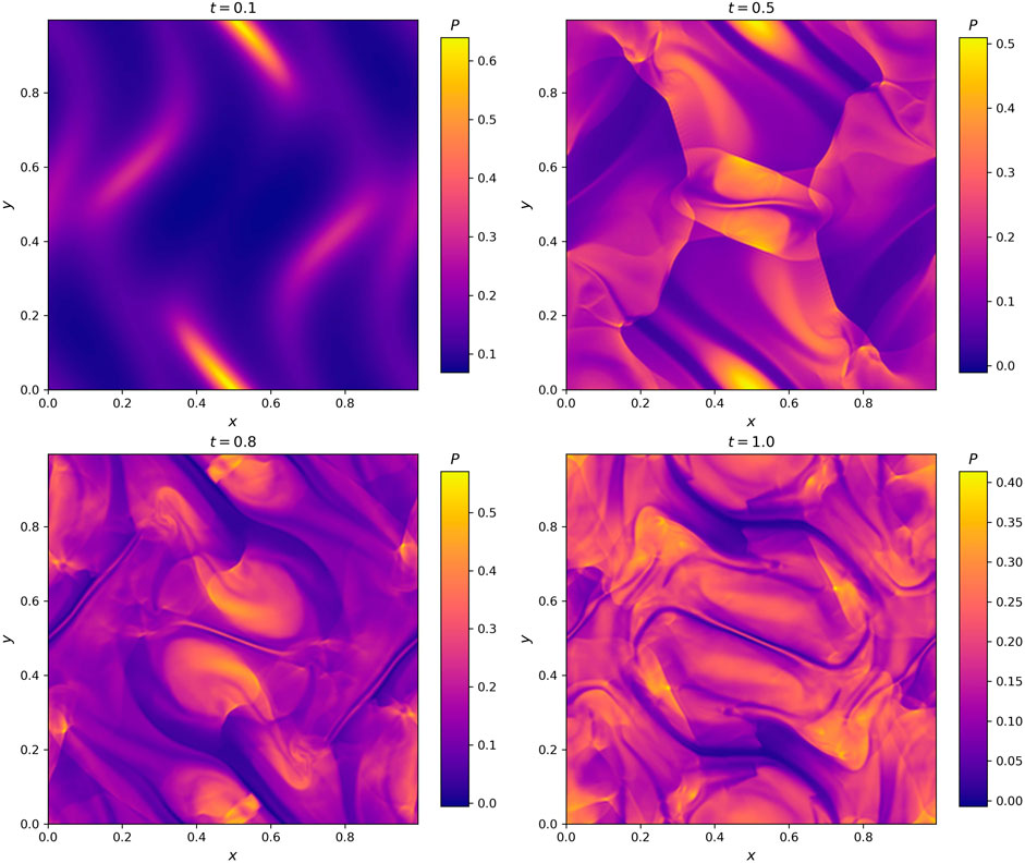
Figure 8. Snapshots of the simulation domain color-coded with thermal pressure P in the Orszag-Tang vortex test. From top left to bottom right are t = 0.1, 0.5, 0.8, and 1.0 respectively. This test has parameter α = 0.49 for the numerical filter.

Figure 9

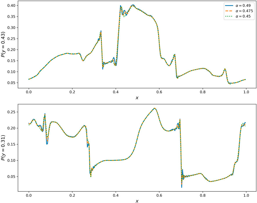
Figure 9. 1D profile of thermal pressure along x at y = 0.43 (top) and y = 0.31 (bottom) at t = 0.5. Different curves correspond to different levels of numerical filtering controlled by the parameter α (Eq. 9).

Figure 10

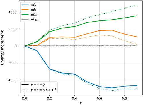
Figure 10. Time evolution of the increment of kinetic energy (blue), magnetic energy (orange), internal energy (green), and total energy (black and white) in the Orszag-Tang vortex test. Solid lines are the run with α= 0.49and without explicit viscosity and resistivity. Dotted lines are the run with α= 0.49and ν= η= 10^–3.

As discussed in Section 2.1, the integrated total energy should be conserved in the compressible simulations. To verify this, we calculate the integrated kinetic energy $(\frac{1}{2}\rho U^2)$, magnetic energy $(\frac{1}{2}{B}^2)$, internal energy (P/(γ − 1)), and total energy (sum of the three energies). In Figure 10, we show the time evolution of the increment (with respect to the initial status) of these energies. Solid lines are the run with α = 0.49 and without explicit viscosity and resistivity. To prove that including viscosity and resistivity does not break the total energy conservation, we conduct one more simulation with α = 0.49 and ν = η = 10^–3. Results of this run are shown as dashed lines. One can see that in both of the two runs, the total energy is exactly conserved (ΔE_tot ≡ 0). Due to diffusion effect, in the run with finite viscosity and resistivity, the magnetic energy and kinetic energy are lower than the run without viscosity and resistivity. However, the internal energy is higher in this run such that the total energy remains unchanged.

4.4 Parametric decay instability

A circularly-polarized Alfvén wave is susceptible to the growth of parametric decay instability (PDI), which breaks the forward propagating Alfvén wave into a forward propagating sound wave and a backward propagating Alfvén wave. Growth of PDI is a compressive process and thus serves as a good test for compressible MHD codes. Here we conduct a 1D simulation using the compressible version of LAPS. The domain size is L_x = 128 and the number of grid is N_x = 4,096. No numerical filter is activated and only the de-aliasing takes effect. Besides, viscosity and resistivity are both zero to avoid effect of diffusion on the growth rate of PDI. The simulation is initialized with a uniform background magnetic field ${\mathit{B}}_{\mathbf{0}}=B_0{\widehat{e}}_x$ with B₀ = 1, a uniform density ρ = 1, and a uniform thermal pressure p = 0.1, i.e., β = 0.2. We set C_t = 0.5 and the resultant Δt is roughly 1.5 × 10⁻². A monochromatic circularly polarized Alfvén wave is added:

$\mathit{U}\left(x\right)=\mathrm{\Delta }B\left[\cos \left(2\pi x\right){\widehat{e}}_y+\sin \left(2\pi x\right){\widehat{e}}_z\right],\mathit{B}\left(x\right)={\mathit{B}}_{\mathbf{0}}-\mathit{U}\left(x\right)(17)$

with ΔB = 0.1. Random fluctuations in density are added on modes with wavelengths between 2 and 1/4.

In Figure 11, we show the evolution of density ρ(x) at three different time moments. One can see that the amplitude of the density fluctuation increases with time. At t = 40, coherent wave packets develop, implying the growth of a narrow range of dominating wave modes. At t = 80, the instability enters nonlinear stage with nearly all wave modes exited. In Panel a) of Figure 12, we show time evolution of density fluctuations on wave modes from k = 1.36 (purple) to k = 1.47 (yellow). There is a clear linear growing phase between t ≈ 20 and t ≈ 60, so we apply linear fit between t = 30 and t = 50 to calculate the growth rate of the density fluctuations. In panel b), the blue curve shows the estimated growth rate as a function of the wavenumber from the simulation result. ω₀ = 1 and k₀ = 1 are the frequency and wavenumber of the mother wave. The orange curve shows the theory prediction of the growth rate of PDI for a circularly-polarized monochromatic Alfvén wave by solving the equation (Derby Jr, 1978)

$\left(\omega +k+2\right)\left(\omega +k-2\right)\left(\omega -k\right)\left({\omega }^2-\tilde{\beta }{k}^2\right)-A^2{k}^2\left({\omega }^3+k{\omega }^2-3\omega +k\right)=0.(18)$

Here A = ΔB/B₀ is the normalized amplitude of the mother wave, $\tilde{\beta }$ is the square of the ratio between sound speed and Alfvén speed and is 1/6 in this case. We can see that the simulation result is consistent with the theory predication.

Figure 11

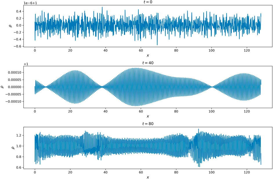
Figure 11. Profiles of density at t = 0 (top), 40 (middle), and 80 (bottom) in the 1D compressible simulation of a monochromatic circularly polarized Alfvén wave.

Figure 12

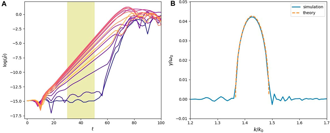
Figure 12. Result of the 1D simulation of parametric decay instability. (A) Time evolution of the amplitude of density fluctuations with wavenumbers from 1.36 (purple) to 1.47 (yellow). The yellow shade marks the time interval for linear fitting. (B) Growth rate as a function of wavenumber estimated from the simulation result (blue) and theory prediction (orange) based on Eq. 18.

5 Summary

In this paper, we present the recently developed 3D Hall-MHD code LAPS (UCLA-Pseudo-Spectral), which is a Fourier transform based pseudo-spectral code and has the expanding-box-model implemented. The code adopts a “pencil” parallelization strategy and has an extremely high scalability. We present test simulations of four benchmark physics problems, including 1) incompressible Hall-MHD waves, 2) incompressible tearing mode instability, 3) Orszag-Tang vortex test, and 4) parametric decay instability of a monochromatic circularly polarized Alfvén wave. The simulation results are well consistent with theory predictions and previous studies, indicating that LAPS is able to simulate Hall-MHD, incompressible-MHD, and compressible-MHD problems with extremely high accuracy. We note that, in this paper, we do not present test results of the expanding-box module. In (Shi et al., 2020b), we introduced the EBM in detail and presented a test simulation on the formation of corotating-interaction-region. Simulations of plasma turbulence conducted using LAPS with EBM were discussed in (Shi et al., 2020b; 2022; Artemyev et al., 2022; Shi et al., 2023). In conclusion, LAPS is a powerful tool in numerical studies of all kinds of MHD and Hall-MHD processes. As a pseudo-spectral code, it is able to resolve all scales with perfect accuracy. Together with the EBM, it is very useful in numerical investigations of turbulence in the expanding solar wind.

Data availability statement

The raw data supporting the conclusion of this article will be made available by the authors, without undue reservation.

Author contributions

CS: Conceptualization, Formal Analysis, Funding acquisition, Methodology, Software, Visualization, Writing–original draft, Writing–review and editing. AT: Conceptualization, Funding acquisition, Methodology, Writing–review and editing. AR: Conceptualization, Methodology, Writing–review and editing. MV: Conceptualization, Funding acquisition, Project administration, Supervision, Writing–review and editing.

Funding

The author(s) declare that financial support was received for the research, authorship, and/or publication of this article. This work is supported by NSF SHINE #2229566 and NASA ECIP #80NSSC23K1064.

Acknowledgments

The development and tests of the code were conducted with the aid of Extreme Science and Engineering Discovery Environment (XSEDE) EXPANSE (allocation No. TG-AST200031) at San Diego Supercomputer Center (SDSC), which is supported by National Science Foundation grant number ACI-1548562 (Towns et al., 2014), and Derecho: HPE Cray EX System (https://doi.org/10.5065/qx9a-pg09) of Computational and Information Systems Laboratory (CISL), National Center for Atmospheric Research (NCAR) (allocation No. UCLA0063).

Conflict of interest

The authors declare that the research was conducted in the absence of any commercial or financial relationships that could be construed as a potential conflict of interest.

Publisher’s note

All claims expressed in this article are solely those of the authors and do not necessarily represent those of their affiliated organizations, or those of the publisher, the editors and the reviewers. Any product that may be evaluated in this article, or claim that may be made by its manufacturer, is not guaranteed or endorsed by the publisher.

Footnotes

¹https://github.com/chenshihelio/LAPS

²https://doi.org/10.5065/qx9a-pg09

References

Artemyev, A., Shi, C., Lin, Y., Nishimura, Y., Gonzalez, C., Verniero, J., et al. (2022). Ion kinetics of plasma flows: earth’s magnetosheath versus solar wind. Astrophysical J. 939, 85. doi:10.3847/1538-4357/ac96e4

CrossRef Full Text | Google Scholar

Brandenburg, A., Johansen, A., Bourdin, P. A., Dobler, W., Lyra, W., Rheinhardt, M., et al. (2021). The pencil code, a modular mpi code for partial differential equations and particles: multipurpose and multiuser-maintained. J. Open Source Softw. 6, 2807. doi:10.21105/joss.02807

CrossRef Full Text | Google Scholar

De Moura, C. A., and Kubrusly, C. S. (2013). The courant–friedrichs–lewy (cfl) condition. AMC 10, 45–90. doi:10.1007/978-0-8176-8394-8

CrossRef Full Text | Google Scholar

Derby Jr, N. F. (1978). Modulational instability of finite-amplitude, circularly polarized alfven waves. Astrophysical J. Part 224 (15), 1013–1016. doi:10.1086/156451

CrossRef Full Text | Google Scholar

Dong, Y., Verdini, A., and Grappin, R. (2014). Evolution of turbulence in the expanding solar wind, a numerical study. Astrophysical J. 793, 118. doi:10.1088/0004-637x/793/2/118

CrossRef Full Text | Google Scholar

Dorfman, S., Zhang, K., Turc, L., Ganse, U., and Palmroth, M. (2023). Probing the foreshock wave boundary with single spacecraft techniques. J. Geophys. Res. Space Phys. 128, e2023JA031724. doi:10.1029/2023ja031724

CrossRef Full Text | Google Scholar

Dormand, J. R., and Prince, P. J. (1980). A family of embedded Runge-Kutta formulae. J. Comput. Appl. Math. 6, 19–26. doi:10.1016/0771-050x(80)90013-3

CrossRef Full Text | Google Scholar

Eymard, R., Gallouët, T., and Herbin, R. (2000). Finite volume methods. Handb. Numer. analysis 7, 713–1018. doi:10.1016/s1570-8659(00)07005-8

CrossRef Full Text | Google Scholar

Frigo, M., and Johnson, S. G. (2005). The design and implementation of fftw3. Proc. IEEE 93, 216–231. doi:10.1109/jproc.2004.840301

CrossRef Full Text | Google Scholar

Furth, H. P., Killeen, J., and Rosenbluth, M. N. (1963). Finite-resistivity instabilities of a sheet pinch. Phys. Fluids 6, 459–484. doi:10.1063/1.1706761

CrossRef Full Text | Google Scholar

Grappin, R., and Velli, M. (1996). Waves and streams in the expanding solar wind. J. Geophys. Res. Space Phys. 101, 425–444. doi:10.1029/95ja02147

CrossRef Full Text | Google Scholar

Hellinger, P., Trávníček, P., Mangeney, A., and Grappin, R. (2003). Hybrid simulations of the expanding solar wind: temperatures and drift velocities. Geophys. Res. Lett. 30. doi:10.1029/2002gl016409

CrossRef Full Text | Google Scholar

Innocenti, M. E., Tenerani, A., and Velli, M. (2019). A semi-implicit particle-in-cell expanding box model code for fully kinetic simulations of the expanding solar wind plasma. Astrophysical J. 870, 66. doi:10.3847/1538-4357/aaf1be

CrossRef Full Text | Google Scholar

Jia, X., Hansen, K. C., Gombosi, T. I., Kivelson, M. G., Tóth, G., DeZeeuw, D. L., et al. (2012). Magnetospheric configuration and dynamics of saturn’s magnetosphere: a global mhd simulation. J. Geophys. Res. Space Phys. 117. doi:10.1029/2012ja017575

CrossRef Full Text | Google Scholar

Kawazura, Y. (2022). Calliope: pseudospectral shearing magnetohydrodynamics code with a pencil decomposition. Astrophysical J. 928, 113. doi:10.3847/1538-4357/ac4f63

CrossRef Full Text | Google Scholar

Lele, S. K. (1992). Compact finite difference schemes with spectral-like resolution. J. Comput. Phys. 103, 16–42. doi:10.1016/0021-9991(92)90324-r

CrossRef Full Text | Google Scholar

Liewer, P. C., Velli, M., and Goldstein, B. E. (2001). Alfvén wave propagation and ion cyclotron interactions in the expanding solar wind: one-dimensional hybrid simulations. J. Geophys. Res. Space Phys. 106, 29261–29281. doi:10.1029/2001ja000086

CrossRef Full Text | Google Scholar

Lin, Y., Wang, X., Lu, S., Perez, J., and Lu, Q. (2014). Investigation of storm time magnetotail and ion injection using three-dimensional global hybrid simulation. J. Geophys. Res. Space Phys. 119, 7413–7432. doi:10.1002/2014ja020005

CrossRef Full Text | Google Scholar

Londrillo, P., and Del Zanna, L. (2000). High-order upwind schemes for multidimensional magnetohydrodynamics. Astrophysical J. 530, 508–524. doi:10.1086/308344

CrossRef Full Text | Google Scholar

Markidis, S., Lapenta, G., and Rizwan-uddin, (2010). Multi-scale simulations of plasma with ipic3d. Math. Comput. Simul. 80, 1509–1519. doi:10.1016/j.matcom.2009.08.038

CrossRef Full Text | Google Scholar

Mignone, A., Bodo, G., Massaglia, S., Matsakos, T., Tesileanu, O. e., Zanni, C., et al. (2007). Pluto: a numerical code for computational astrophysics. Astrophysical J. Suppl. Ser. 170, 228–242. doi:10.1086/513316

CrossRef Full Text | Google Scholar

Mininni, P. D., Rosenberg, D., Reddy, R., and Pouquet, A. (2011). A hybrid mpi–openmp scheme for scalable parallel pseudospectral computations for fluid turbulence. Parallel Comput. 37, 316–326. doi:10.1016/j.parco.2011.05.004

CrossRef Full Text | Google Scholar

Miyoshi, T., and Kusano, K. (2005). A multi-state hll approximate riemann solver for ideal magnetohydrodynamics. J. Comput. Phys. 208, 315–344. doi:10.1016/j.jcp.2005.02.017

CrossRef Full Text | Google Scholar

Orszag, S. A., and Tang, C.-M. (1979). Small-scale structure of two-dimensional magnetohydrodynamic turbulence. J. Fluid Mech. 90, 129–143. doi:10.1017/s002211207900210x

CrossRef Full Text | Google Scholar

Palmroth, M., Ganse, U., Pfau-Kempf, Y., Battarbee, M., Turc, L., Brito, T., et al. (2018). Vlasov methods in space physics and astrophysics. Living Rev. Comput. Astrophysics 4, 1. doi:10.1007/s41115-018-0003-2

PubMed Abstract | CrossRef Full Text | Google Scholar

Pekurovsky, D. (2012). P3dfft: a framework for parallel computations of fourier transforms in three dimensions. SIAM J. Sci. Comput. 34, C192–C209. doi:10.1137/11082748x

CrossRef Full Text | Google Scholar

Perez, J. C., and Chandran, B. D. (2013). Direct numerical simulations of reflection-driven, reduced magnetohydrodynamic turbulence from the sun to the alfvén critical point. Astrophysical J. 776, 124. doi:10.1088/0004-637x/776/2/124

CrossRef Full Text | Google Scholar

Pucci, F., and Velli, M. (2013). Reconnection of quasi-singular current sheets: the “ideal” tearing mode. Astrophysical J. Lett. 780, L19. doi:10.1088/2041-8205/780/2/l19

CrossRef Full Text | Google Scholar

Reuter, K., Jenko, F., Forest, C. B., and Bayliss, R. A. (2008). A parallel implementation of an mhd code for the simulation of mechanically driven, turbulent dynamos in spherical geometry. Comput. Phys. Commun. 179, 245–249. doi:10.1016/j.cpc.2008.02.011

CrossRef Full Text | Google Scholar

Réville, V., Velli, M., Panasenco, O., Tenerani, A., Shi, C., Badman, S. T., et al. (2020). The role of alfvén wave dynamics on the large-scale properties of the solar wind: comparing an mhd simulation with parker solar probe e1 data. Astrophysical J. Suppl. Ser. 246, 24. doi:10.3847/1538-4365/ab4fef

CrossRef Full Text | Google Scholar

Shi, C. (2022). Instabilities in a current sheet with plasma jet. J. Plasma Phys. 88, 555880401. doi:10.1017/s0022377822000575

CrossRef Full Text | Google Scholar

Shi, C., Sioulas, N., Huang, Z., Velli, M., Tenerani, A., and Réville, V. (2023) Evolution of mhd turbulence in the expanding solar wind: residual energy and intermittency. arXiv preprint arXiv:2308.12376.

Google Scholar

Shi, C., Velli, M., Panasenco, O., Tenerani, A., Réville, V., Bale, S. D., et al. (2021). Alfvénic versus non-alfvénic turbulence in the inner heliosphere as observed by parker solar probe. Astronomy Astrophysics 650, A21. doi:10.1051/0004-6361/202039818

CrossRef Full Text | Google Scholar

Shi, C., Velli, M., Pucci, F., Tenerani, A., and Innocenti, M. E. (2020a). Oblique tearing mode instability: guide field and hall effect. Astrophysical J. 902, 142. doi:10.3847/1538-4357/abb6fa

CrossRef Full Text | Google Scholar

Shi, C., Velli, M., Tenerani, A., Rappazzo, F., and Réville, V. (2020b). Propagation of alfvén waves in the expanding solar wind with the fast–slow stream interaction. Astrophysical J. 888, 68. doi:10.3847/1538-4357/ab5fce

CrossRef Full Text | Google Scholar

Shi, C., Velli, M., Tenerani, A., Réville, V., and Rappazzo, F. (2022). Influence of the heliospheric current sheet on the evolution of solar wind turbulence. Astrophysical J. 928, 93. doi:10.3847/1538-4357/ac558b

CrossRef Full Text | Google Scholar

Shoda, M., Suzuki, T. K., Asgari-Targhi, M., and Yokoyama, T. (2019). Three-dimensional simulation of the fast solar wind driven by compressible magnetohydrodynamic turbulence. Astrophysical J. Lett. 880, L2. doi:10.3847/2041-8213/ab2b45

CrossRef Full Text | Google Scholar

Tenerani, A., and Velli, M. (2017). Evolving waves and turbulence in the outer corona and inner heliosphere: the accelerating expanding box. Astrophysical J. 843, 26. doi:10.3847/1538-4357/aa71b9

CrossRef Full Text | Google Scholar

Tenerani, A., Velli, M., Matteini, L., Réville, V., Shi, C., Bale, S. D., et al. (2020). Magnetic field kinks and folds in the solar wind. Astrophysical J. Suppl. Ser. 246, 32. doi:10.3847/1538-4365/ab53e1

CrossRef Full Text | Google Scholar

Tóth, G., Van der Holst, B., Sokolov, I. V., De Zeeuw, D. L., Gombosi, T. I., Fang, F., et al. (2012). Adaptive numerical algorithms in space weather modeling. J. Comput. Phys. 231, 870–903. doi:10.1016/j.jcp.2011.02.006

CrossRef Full Text | Google Scholar

Towns, J., Cockerill, T., Dahan, M., Foster, I., Gaither, K., Grimshaw, A., et al. (2014). Xsede: accelerating scientific discovery. Comput. Sci. Eng. 16, 62–74. doi:10.1109/mcse.2014.80

CrossRef Full Text | Google Scholar

van der Holst, B., Sokolov, I. V., Meng, X., Jin, M., Manchester IV, W. B., Toth, G., et al. (2014). Alfvén wave solar model (awsom): coronal heating. Astrophysical J. 782, 81. doi:10.1088/0004-637x/782/2/81

CrossRef Full Text | Google Scholar

Van der Houwen, P. (1972). Explicit Runge-Kutta formulas with increased stability boundaries. Numer. Math. 20, 149–164. doi:10.1007/bf01404404

CrossRef Full Text | Google Scholar

Virtanen, P., Gommers, R., Oliphant, T. E., Haberland, M., Reddy, T., Cournapeau, D., et al. (2020). Scipy 1.0: fundamental algorithms for scientific computing in python. Nat. methods 17, 261–272. doi:10.1038/s41592-019-0686-2

PubMed Abstract | CrossRef Full Text | Google Scholar

Wray, A. A. (1990) Minimal storage time advancement schemes for spectral methods. California: NASA Ames Research Center. Report No. MS 202.

Google Scholar