A robust numerical scheme for singularly perturbed differential equations with spatio-temporal delays

In this article, we proposed and analyzed a numerical scheme for singularly perturbed differential equations with both spatial and temporal delays. The presence of the perturbation parameter exhibits strong boundary layers, and the large negative shift gives rise to a strong interior layer in the solution. The abruptly changing behaviors of the solution in the layers make it difficult to solve the problem analytically. Standard numerical methods do not give satisfactory results, unless a large mesh number is considered, which needs a massive computational cost. We treated such problem by proposing a numerical scheme using the implicit Euler method in the temporal variable and the nonstandard finite difference method in the spatial variable on uniform meshes. The stability and uniform convergence of the proposed scheme have been investigated and proved. To demonstrate the theoretical results, numerical experiments are carried out. From the theoretical and numerical results, we observed that the method is uniformly convergent of order one in time and of order two in space.

1. Introduction

Delay differential equations are equations that are dependent on the previous states and have been used in various dynamical systems. For instance, in robotics, delays occur through the manipulation of information or feedback control [1]. A surface acoustic wave sensor is modeled using a delay differential equation [2]. In chemical kinetics, the reaction time and the time taken for mixing the reactants are modeled by delay differential equations [3]. Apart from these, delayed dynamical systems have also been found useful in modeling musical instruments [4], traffic dynamics [5], models of HIV infection [6], population dynamics [7], economic cycles [8], and others.

A subclass of differential equations in which the term with the highest order derivative is multiplied by a small positive parameter (ε) and involves one or more shift arguments is said to be a singularly perturbed differential equation with delay [9]. Such problems frequently arise in the modeling of various physical systems, such as the human pupil-light reflex [10], the study of bistable devices in digital electronics [11], variational problem in control theory [12], immune response modeling [13], mathematical modeling in ecology [14], models to stabilize rotating and frozen waves [15], models for the physiological process [16]. The presence of the small positive number causes boundary layers and the spatial delay gives rise to an interior layer in the solution of the problem. The layers are asymptotically narrow regions in the neighborhood of the end points of the domain, where the gradient of the solution decreases as ε approaches zero [17]. The rapidly changing behavior of the solution in the layers causes a significant error in the solution, and hence, it is almost impossible to solve the problem analytically. On the contrary, standard numerical methods do not give satisfactory solutions, unless a large number of mesh points are considered, which requires a massive computational cost [18]. To overcome such drawbacks, there is a need of developing a numerical scheme, independent of the perturbation parameter.

Various research works are available in the literature to address the aforementioned limitations. For instance, Erdogan and Cen [19] solved a singularly perturbed convection–diffusion with delay by constructing a hybrid finite difference scheme on a Shishkin-type mesh and obtained a uniformly convergent method with respect to ε. In [20], a class of turning point singularly perturbed boundary value problems is treated by constructing a numerical scheme based on the trigonometric quintic B-spline basis functions on a piece-wise uniform mesh. The method is obtained to be almost first-order convergent irrespective of ε. In [21], a time-dependent singularly perturbed differential equation with delay is solved by constructing a numerical scheme using the Euler scheme on uniform time mesh and a hybrid finite difference scheme on piece-wise uniform Shishkin mesh in the spatial direction. In [22], two-dimensional singularly perturbed semi-linear convection–diffusion problems have been treated using the nonstandard finite difference approach. The authors linearized the continuous problem and then discretized it using the nonstandard finite difference methods. Mbroh and Munyakazi [23] solved singularly perturbed one- and two-dimensional problems by constructing a scheme using the method of lines by using the fitted operator finite difference method for the space discretization and the Crank–Nicolson method for the time discretization. In [24], a singularly perturbed problem with time lag is treated by constructing a numerical method using the standard finite difference operators centered in space and implicit in time on a piece-wise uniform mesh. Sahoo and Gupta [25] solved a singularly perturbed problem involving discontinuous convective and source terms by developing a numerical scheme using a first-order accurate, simple upwind scheme on specially designed piece-wise uniform Shishkin meshes. Appadu and Tijani [26] treated a one-dimensional generalized Burgers–Huxley equation by proposing two solutions using the classical finite difference scheme and nonstandard finite difference scheme and obtained that one of the proposed solutions contains a minor error. In [27], a singularly perturbed ordinary differential equation with a large negative shift is treated by developing a numerical scheme using the fitted operator method via domain decomposition.

Singularly perturbed differential equations involving large delays in the spatial variable have been solved by few authors. In [28], a singularly perturbed problem with a large delay is solved by developing a scheme using the Crank–Nicolson method on a temporal mesh and the central difference method on nonuniform Shishkin meshes. Bansal and Sharma [29] formulated a scheme for a singularly perturbed with delay using the implicit Euler on the temporal meshes and standard central difference on nonuniform spatial meshes. Ejere et al. [30] developed a numerical scheme for a time-dependent singularly perturbed differential equation with large spatial delays using the weighted-average method in the temporal direction and the central difference method in the spatial direction on piece-wise uniform Shishkin meshes. Alam and Khan [31] proposed a new numerical algorithm for singularly perturbed differential equations involving the shift and the advance parameters. They used Crank–Nicolson in the time direction and cubic B-spline basis functions on generalized Shishkin mesh in the spatial direction, and by this, they obtained a uniformly convergent scheme of order four in time and almost of order four in space.

In this article, we proposed a robust numerical scheme to solve singularly perturbed differential equations involving spatial and temporal delays. The scheme is developed using the implicit Euler method for the temporal variable and the nonstandard finite difference method for the spatial variable on uniform meshes. To handle the temporal delay, we used the Taylor series approximation, and the spatial delay is handled by choosing special meshes, in such a way that the term with the spatial delay coincides with the mesh point x_i = 1. Error estimate and uniform convergence analysis are investigated and proved for the proposed method. Model numerical examples are also solved to support the theoretical results.

The remaining sections of the article are organized as follows: The description of the continuous problem is presented in Section 2. The time semi-discrete scheme and the fully discrete scheme are briefly discussed in Section 3. To support the validity of the proposed scheme, numerical examples, results, and discussions are provided in Section 4, and the study is concluded in Section 5.

Notations: Throughout this article, we used C as a generic positive number, independent of ε and the mesh numbers. If w is the smooth function in $\bar{{D}}$, then we used the maximum norm as $\left|\right|w\left|\right|=\underset{(s,t)\in \bar{{D}}}{max}\left|w(s,t)\right|$.

2. Description of the continuous problem

We considered a singularly perturbed delay differential equation given by

$\begin{array}{ll}\{\begin{array}{l}{{L}}_{\epsilon }w(s,t)=\left(\frac{\partial }{\partial t}-\epsilon \frac{{\partial }^2}{\partial s^2}+\alpha (s)\right)w(s,t)\hfill \\ =\gamma (s,t)-\beta (s)w(s-1,t-\tau ),(s,t)\in {D},\hfill \\ w(s,t)=w_0(s,t),(s,t)\in {{D}}_0=\{(s,t):s\in [0,2],t\in [-\tau ,0]\},\hfill \\ w(s,t)=\psi (s,t),(s,t)\in {{D}}_L=\{(s,t):s\in [-1,0],t\in [0,T]\},\hfill \\ w(2,t)=\phi (t),(2,t)\in {{D}}_R=\{(2,t),t\in [0,T]\},\hfill \end{array}& (1)\end{array}$

Where $\bar{{D}}=\left[0,2\right]\times \left[0,T\right]$, 0 < ε≪1, a temporal shift τ > 0 of o(ε) and a finite time T. We assumed that the functions α(s), β(s), γ(s, t), w₀(s, t), ψ(s, t), and φ(t) are smooth enough and bounded on the considered domain. Moreover, to avoid oscillation in the solution for arbitrary positive constant λ, the coefficient functions α(s) and β(s) satisfy the conditions [29]

$\begin{array}{ll}\alpha (s)+\beta (s)\ge 2\lambda >0\text{ and }\beta (s)<0,s\in \left[0,2\right].& (2)\end{array}$

Setting ε = 0, the associated reduced problem is given by

${{L}}_{0}w(s,t)=\{\begin{array}{l}\left(\frac{\partial }{\partial t}+\alpha (s)\right)w_0(s,t)=\gamma (s,t)-\beta (s){\psi }_0(s-1,t-\tau ),\hfill \\ (s,t)\in {{D}}_L,\hfill \\ \left(\frac{\partial }{\partial t}+\alpha (s)\right)w_0(s,t)=\gamma (s,t)-\beta (s)w_0(s-1,t-\tau ),\hfill \\ (s,t)\in {{D}}_R.\hfill \end{array}$

Since w₀ need not satisfy the conditions w₀(0, t − τ) = ψ(0, t − τ), w₀(0, t − τ) = ψ(0, 0), w₀(2, t − τ) = φ(2, t), $w_0(1^{-},t)=w_0(1^{+},t)$, and ${(w_0)}_s(1^{-},t)={(w_0)}_s(1^{+},t)$, the solution exhibits two boundary layers and an interior layer at s = 1 [28, 32]. The functions involved in the continuous problem (1) should satisfy Holder continuity and compatibility conditions are imposed at the corner points as

$\begin{array}{ll}\{\begin{array}{l}{w}_0(0,0)=\psi (0,0),\hfill \\ w_0(2,0)=\phi (0)\hfill \end{array}& (3)\end{array}$

and

$\begin{array}{ll}\{\begin{array}{l}\frac{\partial \psi (0,0)}{\partial t}-\epsilon \frac{{\partial }^2{w}_0(0,0)}{\partial s^2}+\alpha (0)w_0(0,0)+\beta (0)w_0(-1,-\tau )=\gamma (0,0),\hfill \\ \frac{\partial \phi (2,0)}{\partial t}-\epsilon \frac{{\partial }^2{w}_0(2,0)}{\partial s^2}+\alpha (2)w_0(2,0)+\beta (2)w_0(1,-\tau )=\gamma (2,0).\hfill \end{array}& (4)\end{array}$

From the aforementioned assumptions and conditions, we observe that the solution involves layers and there exists a constant C independent of ε [33]. So for $(s,t)\in \bar{{D}}$, we have |w(s, t) − w₀(s, 0)| = |w(s, t) − w₀(s)| ≤ Ct. Applying Taylor's series expansion, we have

$\begin{array}{ll}w(s-1,t-\tau )=w(s-1,t)-\tau \frac{\partial w(s-1,t)}{\partial t}+O({\tau }^2)& (5)\end{array}$

Inserting Equations (5) into (1) gives

$\begin{array}{ll}{{L}}_{\epsilon }w(s,t)=\vartheta (s,t)(s,t)\in \bar{{D}}& (6)\end{array}$

subjected to

$\begin{array}{ll}\{\begin{array}{l}w(s,t)=w_0(s,t),(s,t)\in \overline{{D}}\hfill \\ w(s,t)=\psi (s,t),(s,t)\in {{D}}_L=\{(s,t):s\in [-1,0],t\in [0,T]\}\hfill \\ w(2,t)=\phi (t),(2,t)\in {{D}}_R=\{(2,t),t\in [0,T]\},\hfill \end{array}& (7)\end{array}$

where

$\begin{array}{l}{{L}}_{\epsilon }w(s,t)=\frac{\partial w(s,t)}{\partial t}-\epsilon \frac{{\partial }^{2}w(s,t)}{\partial s^2}+\alpha (s)w(s,t)\\ \vartheta (s,t)=\{\begin{array}{l}\gamma (s,t)-\beta (s)\psi (s-1,t)+\tau \beta (s)\frac{\partial \psi (s-1,t)}{\partial t},s\in (0,1]\hfill \\ \gamma (s,t)-\beta (s)w(s-1,t)+\tau \beta (s)\frac{\partial w(s-1,t)}{\partial t},s\in (1,2).\hfill \end{array}\end{array}$

Lemma 1. Suppose z(s, t) is a smooth function in $\bar{{D}}$. If z(s, t) ≥ 0, $(s,t)\in \partial {D}$ and ${{L}}_{\epsilon }z(s,t)\ge 0$, $(s,t)\in {D}$, then ${{L}}_{\epsilon }z(s,t)\ge 0$, $(s,t)\in \bar{{D}}$.

Proof. For $(ŝ,\widehat{t})\in \bar{{D}}$, suppose that $z(ŝ,\widehat{t})=\underset{\bar{{D}}}{min}z(s,t)<0$. From the considered hypothesis $(ŝ,\widehat{t})\notin \partial {D}$. By extreme value theorem, we have $z_t(ŝ,\widehat{t})=0,z_s(ŝ,\widehat{t})=0$, and $z_{ss}(ŝ,\widehat{t})>0$. Then,

Case 1: For s ∈ (0, 1], ${{L}}_{\epsilon }z(ŝ,\widehat{t})=\frac{\partial z(ŝ,\widehat{t})}{\partial t}-\epsilon \frac{{\partial }^{2}z(ŝ,\widehat{t})}{\partial s^2}+\alpha (ŝ,\widehat{t})<0.$

Case 2: For s ∈ (1, 2), ${{L}}_{\epsilon }z(ŝ,\widehat{t})=\frac{\partial z(ŝ,\widehat{t})}{\partial t}-\epsilon \frac{{\partial }^{2}z(ŝ,\widehat{t})}{\partial s^2}+\alpha (ŝ)+\beta (ŝ)z(ŝ-1,\widehat{t})-\tau \beta (ŝ)\frac{\partial z(ŝ-1,\widehat{t})}{\partial t}\le \frac{\partial z(ŝ,\widehat{t})}{\partial t}-\epsilon \frac{{\partial }^{2}z(ŝ,\widehat{t})}{\partial s^2}+\left[\alpha (ŝ)+\beta (ŝ)\right]z(ŝ,\widehat{t})-\tau \beta (ŝ)\frac{\partial z(ŝ,\widehat{t})}{\partial t}<0.$

Thus, ${{L}}_{\epsilon }z(ŝ,\widehat{t})<0$, which contradicts the given condition. Therefore, our supposition fails, so that $z(ŝ,\widehat{t})\ge 0$, which implies that z(s, t) ≥ 0, $(s,t)\in \bar{{D}}$. □

Lemma 2. The solution of the continuous problem (6)-(7) is estimated as follows:

$\begin{array}{l}\left|w(s,t)\right|\le \frac{\left|\right|\vartheta \left|\right|}{\lambda }+max\left\{\left|\partial {D}\right|\right\}\end{array}$

Proof. Let us define $z^{\pm }(s,t)=\frac{\left|\right|\vartheta \left|\right|}{\lambda }+max\left\{\left|\partial {D}\right|\right\}\pm w(s,t)$. Then, we have z^±(0, t) ≥ 0 and z^±(0, t) ≥ 0. Moreover, For s ∈ (0, 1], t ∈ [0, T],

$\begin{array}{l}{{L}}_{\epsilon }{z}^{\pm }(s,t)=\left(\frac{\partial }{\partial t}-\epsilon \frac{\partial }{\partial s^2}+\alpha (s)\right)z^{\pm }(s,t)\\ =\alpha (s)\left(\frac{\left|\right|\vartheta \left|\right|}{\lambda }+max\left\{\left|\partial {D}\right|\right\}\right)\pm \vartheta (x,t)\ge 0.\end{array}$

For s ∈ (1, 2), t ∈ [0, T],

$\begin{array}{l}{{L}}_{\epsilon }{z}^{\pm }(s,t)=\left(\frac{\partial }{\partial t}-\epsilon \frac{\partial }{\partial s^2}+\alpha (s)\right)z^{\pm }(s,t)\\ +\beta (s)z^{\pm }(s-1,t)-\tau \beta (s)\frac{\partial z^{\pm }(s-1,t)}{\partial t}\\ \ge \left[\alpha (s)+\beta (s)\right]max\left\{\left|\partial {D}\right|\right\}\ge 0.\end{array}$

Thus, ${{L}}_{\epsilon }{z}^{\pm }(s,t)\ge 0$ and by Lemma 1, we have z^±(s, t) ≥ 0, $(s,t)\in \bar{{D}}$, which yields the stability estimate. □

Lemma 3. The derivatives of the solution w(x, t) of Equations (6), (7) are bounded as follows:

$\left|\frac{{\partial }^{k+l}w(s,t)}{\partial s^k\partial t^l}\right|\le \{\begin{array}{l}C\left(1+{\epsilon }^{-k/2}[e^{-s\sqrt{\lambda /\epsilon }}+e^{-(1-s)\sqrt{\lambda /\epsilon }}]\right),(s,t)\in {{D}}_L,\hfill \\ \hfill \\ C\left(1+{\epsilon }^{-k/2}[e^{-(s-1)\sqrt{\lambda /\epsilon }}+e^{-(2-s)\sqrt{\lambda /\epsilon }}]\right),\hfill \\ (s,t)\in {{D}}_R\hfill \end{array}$

for all nonnegative integer k, l such that 0 ≤ k + 2l ≤ 4.

Proof. For k = 0 and l = 0, it is to show the bound of the solution w(s, t), which is Lemma 2. For k = 0, l ≠ 0, we show the bound of derivatives of w(s, t) with respect to t. For k ≠ 0, l = 0, it is to show the bound of derivatives of the solution w(s, t) with respect to s and for the cases when (k, l) ≠ 0, we determine the bound of its derivatives of the solution w(s, t) with respect to s and t. Let $q_{\epsilon ,1}(s)=e^{-s\sqrt{\lambda /\epsilon }}+e^{-(1-s)\sqrt{\lambda /\epsilon }}$, s ∈ (0, 1] and $q_{\epsilon ,2}(s)=e^{-(s-1)\sqrt{\lambda /\epsilon }}+e^{-(2-s)\sqrt{\lambda /\epsilon }}$, s ∈ (1, 2). For a fixed value of λ, following the approaches of Kellogg and Tsan [34], we can get that |q_{ε, ι}(s)| ≤ c, for constant c and ι = 1, 2. For the case k = 0, Equation (6) becomes

$\begin{array}{l}\frac{\partial w(s,t)}{\partial t}=\epsilon \frac{{\partial }^{2}w(s,t)}{\partial s^2}-\alpha (s)w(s,t)\\ +\{\begin{array}{l}\gamma (s,t)-\beta (s)\psi (s-1,t)+\tau \beta (s)\frac{\partial \psi (s-1,t)}{\partial t},s\in (0,1]\hfill \\ \gamma (s,t)-\beta (s)w(s-1,t)+\tau \beta (s)\frac{\partial w(s-1,t)}{\partial t},s\in (1,2).\hfill \end{array}& (8)\end{array}$

Along the sides t = 0, we have w = 0, which implies that $\frac{{\partial }^{2}w(s,t)}{\partial s^2}=0$. Then from Equation (8), we get

$\begin{array}{l}\frac{\partial w(s,0)}{\partial t}=\epsilon \frac{{\partial }^{2}w(s,0)}{\partial s^2}-\alpha (s)w(s,0)\\ +\{\begin{array}{l}\gamma (s,0)-\beta (s)\psi (s-1,0)+\tau \beta (s)\frac{\partial \psi (s-1,0)}{\partial t},s\in (0,1]\hfill \\ \gamma (s,0)-\beta (s)w(s-1,0)+\tau \beta (s)\frac{\partial w(s-1,0)}{\partial t},s\in (1,2).\hfill \end{array}& (9)\end{array}$

Without loss of generality, assuming that all the values considered in Equation (7) are zero, we have w(s − 1, 0) = ψ(s − 1, 0) = 0, s ∈ [0, 1] and w(s − 1, 0) = w₀(s − 1, 0) = 0, s ∈ (1, 2]. Then, Equation (9) becomes $\frac{\partial w(s,0)}{\partial t}=\gamma (s,0)$. Since γ is a smooth function, it implies ${\displaystyle \left|\frac{\partial w(s,t)}{\partial t}\right|}\le C$, for sufficiently chosen C on $\partial {D}$. Applying the operator ${{L}}_{\epsilon }$ given in Equation (6) on $\frac{\partial w(s,t)}{\partial t}$, we obtain $\left|{{L}}_{\epsilon }{w}_t(s,t)\right|=\left|{\vartheta }_t(s,t)\right|\le C$ on ${D}$. Thus, applying Lemma 1 gives ${\displaystyle \left|\frac{\partial w(s,t)}{\partial t}\right|}\le C$ on $\bar{{D}}$. For l = 2, differentiating Equation (8) with respect to t gives

$\begin{array}{l}\frac{{\partial }^{2}w(s,t)}{\partial t^2}=\epsilon \frac{{\partial }^{3}w(s,t)}{\partial s^2\partial t}-\alpha (s)\frac{\partial w(s,t)}{\partial t}\\ +\{\begin{array}{l}\frac{\partial \gamma (s,t)}{\partial t}-\beta (s)\frac{\partial \psi (s-1,t)}{\partial t}+\tau \beta (s)\frac{{\partial }^2\psi (s-1,t)}{\partial t^2},s\in (0,1]\hfill \\ \frac{\partial \gamma (s,t)}{\partial t}-\beta (s)\frac{\partial w(s-1,t)}{\partial t}+\tau \beta (s)\frac{{\partial }^{2}w(s-1,t)}{\partial t^2},s\in (1,2).\hfill \end{array}& (10)\end{array}$

Along s = 0 and s = 2, we have $\frac{{\partial }^{2}w(s,t)}{\partial t^2}=0$, and along t=0, we have w = 0 and $\frac{{\partial }^{2}w(s,0)}{\partial s^2}=0$. From $\frac{\partial w(s,0)}{\partial t}=\gamma (s,0)$, we have $\frac{{\partial }^{3}w(s,0)}{\partial s^2\partial t}=\frac{{\partial }^2\gamma (s,0)}{\partial s^2}$. Assuming that the initial and boundary conditions are identically zero, we have w_t(s − 1, 0) = ψ_t(s − 1, 0) = 0, s ∈ (0, 1] and w_t(s − 1, 0) = (_w0)t(s − 1, 0) = 0, s ∈ (1, 2]. Then from Equation (10), we get

$\begin{array}{l}\frac{{\partial }^{2}w(s,0)}{\partial t^2}=\epsilon \frac{{\partial }^2\gamma (s,0)}{\partial s^2}-\alpha (s)\frac{\partial \gamma (s,0)}{\partial t}\\ +\{\begin{array}{l}\frac{\partial \gamma (s,0)}{\partial t},s\in (0,1]\hfill \\ \frac{\partial \gamma (s,0)}{\partial t}+\tau \beta (s)\frac{{\partial }^{2}w(s-1,0)}{\partial t^2},s\in (1,2).\hfill \end{array}& (11)\end{array}$

From Equation (11), along t = 0, we obtain that ${\displaystyle \left|\frac{{\partial }^{2}w(s,0)}{\partial t^2}\right|}\le 0$ on $\partial {D}$ and the operator ${{L}}_{\epsilon }$ implies $\left|{{L}}_{\epsilon }\frac{{\partial }^{2}w(s,t)}{\partial t^2}\right|=\left|\frac{{\partial }^2\vartheta (s,t)}{\partial t^2}\right|\le C$ on ${D}$ and applying Lemma 1 yields ${\displaystyle \left|\frac{{\partial }^{2}w(s,t)}{\partial t^2}\right|}\le C$ on $\bar{{D}}$. The bound of derivatives of the solution w(s, t) for the cases k ≠ 0 can be determined by similar procedures as mentioned earlier. For the case k = 1, let $s\in {D}$ and consider a neighborhood $R=(e,e+\sqrt{\epsilon })$, ∀s ∈ R. For some $q\in \bar{R}$ and t ∈ (0, T], the mean value theorem gives

$\begin{array}{ll}{\displaystyle \left|\frac{\partial w(q,t)}{\partial s}\right|}={\epsilon }^{\frac{-1}{2}}|w(e+\sqrt{\epsilon },t)-w(e,t)|\le 2{\epsilon }^{\frac{-1}{2}}\left|\right|w\left|\right|.& (12)\end{array}$

For $s\in \bar{R}$, we can get

$\begin{array}{l}\frac{\partial w(s,t)}{\partial s}=\frac{\partial w(q,t)}{\partial s}+\frac{\partial w(s,t)}{\partial s}-\frac{\partial w(q,t)}{\partial s}\\ =\frac{\partial w(q,t)}{\partial s}+{\displaystyle {\int }_q^s}\frac{\partial w(x,t)}{\partial x}dx=\frac{\partial w(q,t)}{\partial s}\\ +{\epsilon }^{-1}{\displaystyle {\int }_q^s}{\displaystyle (\frac{\partial w(x,t)}{\partial x}+\alpha (x)w(x,t)}\\ {\displaystyle +\beta (x)w(x-1,t)-\gamma (x,t))}dx.\\ \Rightarrow {\displaystyle \left|\frac{\partial w(s,t)}{\partial s}\right|}\le {\displaystyle \left|\frac{\partial w(q,t)}{\partial s}\right|}+C{\epsilon }^{-1}{\displaystyle {\int }_q^s}(\left|\right|w\left|\right|+\left|\right|\gamma \left|\right|)dx\\ ={\displaystyle \left|\frac{\partial w(q,t)}{\partial s}\right|}+C{\epsilon }^{-1}(\left|\right|w\left|\right|+\left|\right|\gamma \left|\right|){\epsilon }^{\frac{1}{2}}.\end{array}$

Putting Equation (12) into the aforementioned result, we obtain ${\displaystyle \left|\frac{\partial w(s,t)}{\partial s}\right|}\le C(1+{\epsilon }^{\frac{-1}{2}}{q}_{\epsilon ,\iota })$, $(s,t)\in \bar{{D}}$ for sufficiently large chosen C. For k = 2, by rearranging Equation (1) we get

$\begin{array}{ll}\frac{{\partial }^{2}w(s,t)}{\partial s^2}={\epsilon }^{-1}\left[\frac{\partial w(s,t)}{\partial t}+\alpha (s)w(s,t)+\beta (s)w(s-1,t)-\gamma (s,t)\right].& (13)\end{array}$

For a fixed time t ∈ [0, T] and for s ∈ [0, 2], since |w| ≤ C, ${\displaystyle \left|\frac{\partial w(s,t)}{\partial t}\right|}\le C$, and γ is a smooth function, $\left|\frac{{\partial }^{2}w(s,t)}{\partial s^2}\right|\le C(1+{\epsilon }^{-1}{q}_{\epsilon ,\iota })$. The derivative of Equation (13) with respect to t gives

$\begin{array}{l}\frac{{\partial }^{3}w(s,t)}{\partial s^2\partial t}={\epsilon }^{-1}{\displaystyle (\frac{{\partial }^{2}w(s,t)}{\partial t^2}+\alpha (s)\frac{\partial w(s,t)}{\partial t}}\\ {\displaystyle +\beta (s)\frac{\partial w(s-1,t)}{\partial t}-\frac{\partial \gamma (s,t)}{\partial t})}.\end{array}$

Since ${\displaystyle \left|\frac{\partial w(s,t)}{\partial t}\right|}\le C$, ${\displaystyle \left|\frac{{\partial }^{2}w(s,t)}{\partial t^2}\right|}\le C$, and |γ_t(s, t)| ≤ C, we get $\left|\frac{{\partial }^{3}w(s,t)}{\partial s^2\partial t}\right|\le C(1+{\epsilon }^{-1}{q}_{\epsilon ,\iota })$. In a similar procedure, the bounds on the derivatives of the solution can be easily determined for the remaining values of k and l with 0 ≤ k + 2l ≤ 4. □

3. Numerical scheme

3.1. Semi-discrete scheme in time direction

Let m be a uniform mesh number on [0, T] with step size Δt. Then, the uniform temporal discretization is given as ${\bar{{D}}}_t^m=\left\{t_j=j\Delta t,\Delta t=T/m,j=0(1)m\right\}$. Using the implicit Euler method, we obtain a semi-discrete scheme as

$\begin{array}{ll}{{L}}_{\epsilon }^m{W}^{j+1}(s)={\vartheta }^{j+1}(s),& (14)\end{array}$

where

${{L}}_{\epsilon }^m{W}^{j+1}(s)=\{\begin{array}{l}-\epsilon \frac{d^2{W}^{j+1}(s)}{d{s}^2}+(\frac{1}{\Delta t}+\alpha (s))W^{j+1}(s),0<s\le 1,\hfill \\ -\epsilon \frac{d^2{W}^{j+1}(s)}{d{s}^2}+(\frac{1}{\Delta t}+\alpha (s))W^{j+1}(s)\hfill \\ +(1-\frac{\tau }{\Delta t})\beta (s)W^{j+1}(s-1),1<s<2\hfill \end{array}$

and

${\vartheta }^{j+1}(s)=\{\begin{array}{l}{\gamma }^{j+1}(s)+\frac{W^j(s)}{\Delta t}-(1-\frac{\tau }{\Delta t})\beta (s){\psi }^{j+1}(s-1)\hfill \\ -\frac{\tau \beta (s)}{\Delta t}{\psi }^j(s-1),s\in (0,1],\hfill \\ {\gamma }^{j+1}(s)+\frac{W^j(s)}{\Delta t}-\frac{\tau \beta (s)}{\Delta t}{W}^j(s-1),s\in (1,2)\hfill \end{array}$

with the initial and boundary conditions

$\begin{array}{ll}\{\begin{array}{l}{W}^0(s)=w_0(s),s\in [0,2],\hfill \\ W^{j+1}(s)={\psi }^{j+1}(s),s\in (0,1],\hfill \\ W^{j+1}(2)={\phi }^{j+1}(2),s\in (1,2).\hfill \end{array}& (15)\end{array}$

Lemma 4. For a smooth function z^j+1(s), suppose that z^j+1(s) ≥ 0, $s\in \partial {D}$ and ${{L}}_{\epsilon }^m{z}^{j+1}(s)\ge 0$, $s\in {D}$. Then, z^j+1(s) ≥ 0, $s\in \bar{{D}}$.

Proof. Let s^* ∈ [0, 2] and suppose that $z^{j+1}(s^{*})=\underset{\bar{{D}}}{min}{z}^{j+1}(s)<0$. By the considered hypothesis, $s^{*}\notin \partial {D}$ and by the extreme value theorem, we have $\frac{d{z}^{j+1}(s^{*})}{ds}=0$ and $\frac{d^2{z}^{j+1}(s^{*})}{d{s}^2}\ge 0$.

Case 1: For s^* ∈ (0, 1], ${{L}}_{\epsilon }^m{z}^{j+1}(s^{*})=-\epsilon \frac{d^2{z}^{j+1}(s^{*})}{d{s}^2}+(\frac{1}{\Delta t}+\alpha (s^{*}))z^{j+1}(s^{*})<0.$

Case 2: For s^* ∈ (1, 2), ${{L}}_{\epsilon }^m{z}^{j+1}(s^{*})=(-\epsilon \frac{d^2}{d{s}^2}+\frac{1}{\Delta t}+\alpha (s^{*}))z^{j+1}(s^{*})+(1-\frac{\tau }{\Delta t})\beta (s^{*})z^{j+1}(s^{*}-1)\le -\epsilon \frac{d^2{z}^{j+1}(s^{*})}{d{s}^2}+(\frac{1}{\Delta t}+\alpha (s^{*})+(1-\frac{\tau }{\Delta t})\beta (s^{*}))z^{j+1}(s^{*})<0.$ The two cases contradict the given condition. Therefore, our assumption is wrong, which implies that z^j+1(s) ≥ 0, $s\in \bar{{D}}$. As a result for the operator ${{L}}_{\epsilon }^m$, we have

$\begin{array}{ll}\left|\right|{({{L}}_{\epsilon }^m)}^{-1}\left|\right|\le {(1+\lambda \Delta t)}^{-1},& (16)\end{array}$

which is used in estimating the truncation error. □

Lemma 5. (Semi-discrete stability estimate) The solution W^j+1(s) of Equations (14), (15) can be estimated as $\left|W^{j+1}(s)\right|\le \frac{\left|\right|{{L}}_{\epsilon }^{m}W\left|\right|}{1+\lambda \Delta t}+max\left\{\left|\partial {{D}}^m\right|\right\}$, s ∈ [0, 2].

Proof. Define two barrier functions as $Z_{\pm }^{j+1}(s)=\frac{\left|\right|{{L}}_{\epsilon }^{m}W\left|\right|}{1+\lambda \Delta t}+max\left\{\left|\partial {{D}}^m\right|\right\}\pm W^{j+1}(s)$, from which we can obtain that $Z_{\pm }^{j+1}(0)\ge 0$ and $Z_{\pm }^{j+1}(2)\ge 0$.

Case 1: For 0 < s ≤ 1, we have

$\begin{array}{l}{{L}}_{\epsilon }^m{Z}_{\pm }^{j+1}(s)=-\epsilon \frac{d^2{Z}_{\pm }^{j+1}}{d{s}^2}+\left(\frac{1}{\Delta t}+\alpha (s)\right)Z_{\pm }^{j+1}(s)\\ =\pm {\vartheta }^{j+1}(s)+\left(\frac{1}{\Delta t}+\alpha (s)\right)\left[\frac{\left|\right|{{L}}_{\epsilon }^{m}W\left|\right|}{1+\lambda \Delta t}+max\left\{\left|\partial {{D}}^m\right|\right\}\right]\\ \ge \left(\frac{1}{\Delta t}+\alpha (s)\right)max\left\{\left|\partial {{D}}^m\right|\right\}\ge 0.\end{array}$

Case 2: For 1 < s < 2, we have

$\begin{array}{l}{{L}}_{\epsilon }^m{Z}_{\pm }^{j+1}(s)=-\epsilon \frac{d^2{Z}_{\pm }^{j+1}}{d{s}^2}+\left(\frac{1}{\Delta t}+\alpha (s)\right)Z_{\pm }^{j+1}(s)\\ +\left(1-\frac{\tau }{\Delta t}\right)\beta (s)Z_{\pm }^{j+1}(s-1)\\ \ge -\epsilon \frac{d^2{Z}_{\pm }^{j+1}}{d{s}^2}+\left(\frac{1}{\Delta t}+\alpha (s)\right)Z_{\pm }^{j+1}(s)\\ +\left(1-\frac{\tau }{\Delta t}\right)\beta (s)Z_{\pm }^{j+1}(s)\\ =\pm {\vartheta }^{j+1}(s)+\left(\frac{1}{\Delta t}+\alpha (s)+\left[1-\frac{\tau }{\Delta t}\right]\beta (s)\right)\\ \left[\frac{\left|\right|{{L}}_{\epsilon }^{m}W\left|\right|}{1+\lambda \Delta t}+max\left\{\left|\partial {{D}}^m\right|\right\}\right]\\ \ge \left(\frac{1}{\Delta t}+\alpha (s)+\left[1-\frac{\tau }{\Delta t}\right]\beta (s)\right)max\left\{\left|\partial {{D}}^m\right|\right\}\ge 0.\end{array}$

Thus, applying Lemma 4 yields $Z_{\pm }^{j+1}(s)\ge 0$, s ∈ [0, 2], which implies the required estimation. □

The local error committed in the semi-discrete scheme is the difference between the exact solution w(s, t_j+1) and the approximate solution W^j+1(s) of Equation (14). That is, $e^{j+1}(s)=w(s,t_{j+1})-W^{j+1}(s)$ and the global error E^j+1 is the contribution of the local error up to the (j + 1)^th time level. The bound of error for the semi-discrete scheme is estimated as follows.

Lemma 6. Suppose that $\left|\frac{{\partial }^{k}w(s,t)}{\partial t^k}\right|\le C$, $(s,t)\in \bar{{D}}$, k = 0, 1, 2. The local error is estimated as $\left|\right|e_{j+1}\left|\right|\le C{(\Delta t)}^2$, and with this condition, the global error is estimated as ||E_j+1|| ≤ C(Δt), j + 1 = 1, 2, …, m.

Proof. From the Taylor series expansion, we have $w^{j+1}(s)=w^j(s)+\Delta t\frac{dw(s,t_j)}{dt}+O({(\Delta t)}^2)$ and from this we obtain

$\begin{array}{ll}\frac{w^{j+1}(s)-w^j(s)}{\Delta t}=\frac{\partial w_t(s,t_j)}{\partial t}+O({(\Delta t)}^2).& (17)\end{array}$

Using Equations (17) into (6) gives

$\begin{array}{ll}{{L}}_{\epsilon }^m{w}^{j+1}(s)+O({(\Delta t)}^2)={\vartheta }^{j+1}(s)& (18)\end{array}$

From Equations (14), (18), we can obtain the boundary value problem of the form

$\begin{array}{ll}{{L}}_{\epsilon }^m{e}^{j+1}(s)=O({(\Delta t)}^2),e^{j+1}(0)=0=e^{j+1}(2)& (19)\end{array}$

Using Equations (16) into (19) yields ||e^j+1|| ≤ C(Δt)². Using the estimation of e^j+1, we have

$\begin{array}{l}\left|\right|E^{j+1}\left|\right|={\displaystyle \left|\right|{\displaystyle \sum _{\xi =1}^j}{e}^{\xi }\left|\right|},j(\Delta t)\le T\\ =\left|\right|e^1+e^2+...+e^j\left|\right|\\ \le \left|\right|e^1\left|\right|+\left|\right|e^2\left|\right|+...+\left|\right|e^{j+1}\left|\right|\\ \le C^{\prime }T(\Delta t)\le C(\Delta t),j+1=1,2,...,m.\end{array}$

Thus, the semi-discrete scheme is convergent of order one in time. □

Lemma 7. Let the solution of Equation (14) be W^j+1(s). Then, its derivatives can be bounded as follows:

$\left|\frac{d^k{W}^{j+1}}{d{s}^k}\right|\le \{\begin{array}{l}{\displaystyle C[1+{\epsilon }^{-k/2}(\exp (-\sqrt{\lambda /\epsilon }s)}\hfill \\ {\displaystyle +\exp (-\sqrt{\lambda /\epsilon }(1-s))\left)\right],s\in [0,1],}\hfill \\ {\displaystyle C[1+{\epsilon }^{-k/2}(\exp (-\sqrt{\lambda /\epsilon }(s-1))}\hfill \\ {\displaystyle +\exp (-\sqrt{\lambda /\epsilon }(2-s))\left)\right],s\in (1,2],}\hfill \end{array}$

where k = 0, 1, 2, 3, 4.

Proof. The proof can be calculated by applying the procedures in the proof of Lemma 3 for the spatial domain. Furthermore, we refer to Clavero and Gracia [35]. □

3.2. Fully-discrete scheme

Let us sub-divide the domain [0, 2] into n uniform meshes of size h, such that ${{D}}_s^N=\left\{0=s_0,s_1,...,s_{n/2}=1,s_{n/2+1},...,s_n=2,s_i=s_0+ih,i=0(1)n,h=2/n\right\}$. According to the procedures in [36], we consider a constant coefficient sub-equation from Equation (14) as

$\begin{array}{ll}-\epsilon \frac{d^2{W}^{j+1}(s)}{d{s}^2}+\lambda W^{j+1}(s)=0,& (20)\end{array}$

Where $\frac{1}{\Delta t}+\alpha (s)\ge \lambda >0$. The characteristic of Equation (20) has two distinct roots $r_1=e^{\sqrt{\frac{\lambda }{\epsilon }}s}$ and $r_2=e^{-\sqrt{\frac{\lambda }{\epsilon }}s}$. Denoting $W_i^{j+1}$ as the approximation of W^j+1(s) at the grid point s_i, we have $W_i^{j+1}=c_1{e}^{\sqrt{\frac{\lambda }{\epsilon }}{s}_i}+c_2{e}^{-\sqrt{\frac{\lambda }{\epsilon }}{s}_i}$ and

$\begin{array}{l}{\displaystyle \left|\begin{array}{ccc}{W}_{i-1}^{j+1}& e^{\sqrt{\frac{\lambda }{\epsilon }}{s}_{i-1}}& e^{-\sqrt{\frac{\lambda }{\epsilon }}{s}_{i-1}}\\ W_i^{j+1}& e^{\sqrt{\frac{\lambda }{\epsilon }}{s}_i}& e^{-\sqrt{\frac{\lambda }{\epsilon }}{s}_i}\\ W_{i+1}^{j+1}& e^{\sqrt{\frac{\lambda }{\epsilon }}{s}_{i+1}}& e^{-\sqrt{\frac{\lambda }{\epsilon }}{s}_{i+1}}\end{array}\right|=0}.\end{array}$

After certain manipulation, we get

$\begin{array}{ll}{W}_{i-1}^{j+1}-2cosh\left(\sqrt{\frac{\lambda }{\epsilon }}h\right)W_i^{j+1}+W_{i+1}^{j+1}=0.& (21)\end{array}$

The finite difference approximation of Equation (20) is given as

$\begin{array}{ll}-\epsilon \frac{W_{i-1}^{j+1}-2W_i^{j+1}+W_{i+1}^{j+1}}{{\sigma }_i^2}+\lambda W_i^{j+1}=0,& (22)\end{array}$

where σ_i is a denominator function. From Equatiosn (21), (22), the denominator function for the variable coefficients is given as

$\begin{array}{ll}{\sigma }_i=\frac{2}{{\omega }_i}sinh\left(\frac{{\omega }_{i}h}{2}\right),\text{ where }{\omega }_i=\sqrt{\frac{1+\Delta t{\alpha }_i}{\epsilon \Delta t}}& (23)\end{array}$

Using the denominator function (Equation 23), we can obtain a fully discrete scheme as

$\begin{array}{ll}{{L}}_{\epsilon }^{n,m}{W}_i^{j+1}={\vartheta }_i^{j+1},i=1,2,...,n-1,& (24)\end{array}$

where

${{L}}_{\epsilon }{W}_i^{j+1}=\{\begin{array}{l}-\epsilon {\delta }^2{W}_i^{j+1}+(\frac{1}{\Delta t}+{\alpha }_i)W_i^{j+1},i=1(1)n/2,\hfill \\ -\epsilon {\delta }^2{W}_i^{j+1}+(\frac{1}{\Delta t}+{\alpha }_i)W_i^{j+1}+(1-\frac{\tau }{\Delta t}){\beta }_i{W}_{i-n/2}^{j+1},\hfill \\ i=n/2+1(1)n-1\hfill \end{array}$

and

${\vartheta }_i^{j+1}=\{\begin{array}{l}{\gamma }_i^{j+1}+\frac{W_i^j}{\Delta t}-(1-\frac{\tau }{\Delta t}){\beta }_i{\psi }_{i-n/2}^{j+1}-\frac{\tau }{\Delta t}{\beta }_i{\psi }_{i-n/2}^j,\hfill \\ i=1(1)n/2,\hfill \\ {\gamma }_i^{j+1}+\frac{W_i^j}{\Delta t}-\frac{\tau }{\Delta t}{\beta }_i{W}_{i-n/2}^j,i=n/2+1(1)n-1,\hfill \end{array}$

With ${\delta }^2{W}_i^{j+1}=\frac{W_{i+1}^{j+1}-2W_i^{j+1}+W_{i-1}^{j+1}}{{\sigma }_i^2}$, and the discrete initial and boundary conditions $W^0(s_i)=w_0(s_i),W^{j+1}(s_i)={\psi }^{j+1}(s_i)$, $W^{j+1}(2)=\phi (2,t_{j+1}),s_i\in \left[0,2\right],t_{j+1}\in \left[0,T\right]$.

Lemma 8. Let $Z_i^{j+1}$ be a given mesh function satisfying $Z_0^{j+1}\ge 0$ and $Z_n^{j+1}\ge 0$. If ${{L}}_{\epsilon }^{n,m}{Z}_i^{j+1}\ge 0$ for i = 1(1)n − 1, then we have $Z_i^{j+1}\ge 0$ for i = 0(1)n.

Proof. For some y ∈ {1, …, n − 1}, suppose that $Z_y^{j+1}=\underset{i=1,...,n-1}{min}{Z}_i^{j+1}<0$.

Case 1: For $y=1,2,...,\frac{n}{2}$, we have ${{L}}_{\epsilon ,1}^n{Z}_y^{j+1}=-\epsilon {\delta }^2{Z}_y^{j+1}+(\frac{1}{\Delta t}+{\alpha }_y)Z_y^{j+1}<0$.

Case 2: For $y=\frac{n}{2}+1,\frac{n}{2}+2,...,n-1$, we have ${{L}}_{\epsilon ,2}^n{Z}_y^{j+1}=-\epsilon {\delta }^2{Z}_y^{j+1}+(\frac{1}{\Delta t}+{\alpha }_y)Z_y^{j+1}+(1-\frac{\tau }{\Delta t}){\beta }_y{Z}_{y-n/2}^{j+1}\le -\epsilon {\delta }^2{Z}_y^{j+1}+(\frac{1}{\Delta t}+{\alpha }_y)Z_y^{j+1}+(1-\frac{\tau }{\Delta t}){\beta }_y{Z}_y<0$. From the two cases, we see that the given hypothesis is contradicted, and hence our assumption fails. Thus, $Z_i^{j+1}\ge 0$, i = 0(1)n. □

Lemma 9. The solution $W_i^{j+1}$ of the fully discrete scheme (24) is estimated as

$\begin{array}{l}\left|W_i^{j+1}\right|\le \frac{\Delta t\left|\right|\vartheta \left|\right|}{1+\lambda \Delta t}+max\left\{\left|\partial {{D}}^{n,m}\right|\right\},i=0(1)n.\end{array}$

Proof. Let us define ${\pi }_{i,\pm }^{j+1}=\frac{\Delta t\left|\right|\vartheta \left|\right|}{1+\lambda \Delta t}+max\left\{\left|\partial {{D}}^{n,m}\right|\right\}\pm W_i^{j+1}$. Then, we have

$\begin{array}{l}{\pi }_{0,\pm }^{j+1}=\frac{\Delta t\left|\right|\vartheta \left|\right|}{1+\lambda \Delta t}+max\left\{\left|\partial {{D}}^{n,m}\right|\right\}\pm W_0^{j+1}\ge \frac{\Delta t\left|\right|\vartheta \left|\right|}{1+\lambda \Delta t}\ge 0\\ {\pi }_{n,\pm }^{j+1}=\frac{\Delta t\left|\right|\vartheta \left|\right|}{1+\lambda \Delta t}+max\left\{\left|\partial {{D}}^{n,m}\right||\right\}\pm W_n^{j+1}\ge \frac{\Delta t\left|\right|\vartheta \left|\right|}{1+\lambda \Delta t}\ge 0\end{array}$

When $i=1(1)\frac{1}{n}$, we obtain

$\begin{array}{l}{{L}}_{\epsilon ,1}^{n,m}{\pi }_{i,\pm }^{j+1}=-\epsilon {\delta }^2{\pi }_{i,\pm }^{j+1}+\left(\frac{1}{\Delta t}+{\alpha }_i\right){\pi }_{i,\pm }^{j+1}\\ =\left(\frac{1}{\Delta t}+{\alpha }_i\right)\left(\frac{\Delta t\left|\right|\vartheta \left|\right|}{1+\lambda \Delta t}+max\left\{\left|\partial {{D}}^{n,m}\right|\right\}\right)\pm {\vartheta }_i^{j+1}\\ \ge \left(\frac{1}{\Delta t}+{\alpha }_i\right)max\left\{\left|\partial {{D}}^{n,m}\right|\right\}\ge 0\end{array}$

When $i=\frac{n}{2}+1(1)n-1$, we obtain

$\begin{array}{l}{{L}}_{\epsilon ,2}^{n,m}{\pi }_{i,\pm }^{j+1}=-\epsilon {\delta }^2{\pi }_{i,\pm }^{j+1}+\left(\frac{1}{\Delta t}+{\alpha }_i\right){\pi }_{i,\pm }^{j+1}+\left(1-\frac{\tau }{\Delta t}\right){\beta }_i{\varphi }_{i-n/2,\pm }^{j+1}\\ =\left(\frac{1}{\Delta t}+{\alpha }_i+\left(1-\frac{\tau }{\Delta t}\right){\beta }_i\right)\\ \left(\frac{\Delta t\left|\right|\vartheta \left|\right|}{1+\lambda \Delta t}+max\left\{\left|\partial {{D}}^{n,m}\right|\right\}\right)\pm {\vartheta }_i^{j+1}\\ \ge \left(1+\Delta t{\alpha }_i+\left(1-\frac{\tau }{\Delta t}\right){\beta }_i\right)max\left\{\left|\partial {{D}}^{n,m}\right|\right\}\ge 0\end{array}$

Thus, applying Lemma 8, we have ${\pi }_{i,\pm }^{j+1}\ge 0$, j = 0(1)n, which yields the stability estimate. □

Lemma 10. For a given fixed mesh number n, we have

$\underset{\epsilon \to 0}{\lim }\{\begin{array}{l}\underset{s_i\in (0,1]}{\max }\frac{\exp \left(-\sqrt{\frac{\alpha (x_i)}{\epsilon }}{s}_i\right)+\exp \left(-\sqrt{\frac{\alpha (s_i)}{\epsilon }}(1-s_i)\right)}{{\epsilon }^{k/2}}=0,\hfill \\ \underset{s_i\in (1,2)}{\max }\frac{\exp \left(-\sqrt{\frac{\alpha (s_i)}{\epsilon }}(s_i-1)\right)+\exp \left(-\sqrt{\frac{\alpha (s_i)}{\epsilon }}(2-s_i)\right)}{{\epsilon }^{k/2}}=0\hfill \end{array}$

for all i = 1(1)n − 1 and k = 1, 2, 3, ….

Proof. We refer to Lemma 3.3 of Woldaregay and Duressa [37]. □

Theorem 1. Let the solution of Equation (14) be W(s, t_j+1) and the solution of (24) be $W_i^{j+1}$. Then, we have

$\begin{array}{l}{\displaystyle \underset{i=0(1)n,j=0(1)m}{max}}|W_i^{j+1}-W(s_i,t_{j+1})|\le C{n}^{-2}.\end{array}$

Proof. From the differential and difference equations, the truncation error is given by

$\begin{array}{l}{\displaystyle \left|{{L}}_{\epsilon }^{n,m}\left(W^{j+1}(s_i)-W_i^{j+1}\right)\right|=|-\epsilon \frac{d^2{W}^{j+1}(s_i)}{d{s}^2}+\epsilon {\delta }^2{W}_i^{j+1}|}\\ {\displaystyle =|-\epsilon \frac{d^2{W}^{j+1}(s_i)}{d{s}^2}+\frac{\epsilon }{{\sigma }_i^2}\left(W_{i+1}^{j+1}-2W_i^{j+1}+W_{i-1}^{j+1}\right)|}& (25)\end{array}$

By the Taylor series expansion of $W_{i+1}^{j+1}$, $W_{i-1}^{j+1}$, and $\frac{1}{{\sigma }_i}$ truncated up to order five, we have

$\begin{array}{l}{W}_{i+1}^{j+1}=W_i^{j+1}+h\frac{d{W}^{j+1}}{ds}+\frac{h^2}{2!}\frac{d^2{W}^{j+1}}{d{s}^2}+\frac{h^3}{3!}\frac{d^3{W}^{j+1}}{d{s}^3}\\ +\frac{h^4}{4!}\frac{d^4{W}^{j+1}({\zeta }_i)}{d{s}^4},{\zeta }_i\in (s_{i-1},s_{i+1}),\\ \end{array}$

$\begin{array}{l}{W}_{i-1}^{j+1}=W_i^{j+1}-h\frac{d{W}^{j+1}}{ds}+\frac{h^2}{2!}\frac{d^2{W}^{j+1}}{d{s}^2}-\frac{h^3}{3!}\frac{d^3{W}^{j+1}}{d{s}^3}\\ +\frac{h^4}{4!}\frac{d^4{W}^{j+1}({\zeta }_i)}{d{s}^4},{\zeta }_i\in (s_{i-1},s_{i+1}),\\ \frac{1}{{\sigma }_i^2}=\frac{{\omega }_i^2}{4{sinh}^2({\omega }_{i}h/2)}=\frac{{\omega }_i^2}{4}\left(\frac{4}{{({\omega }_{i}h)}^2}-\frac{1}{3}+\frac{{({\omega }_{i}h)}^2}{60}\right).\end{array}$

Putting these expansions in Equation (25) yields

$\begin{array}{l}\left|{{L}}_{\epsilon }^{n,m}\left(W^{j+1}(s_i)-W_i^{j+1}\right)\right|\\ =|-\epsilon \frac{d^2{W}_i^{j+1}}{d{s}^2}+\epsilon \frac{d^2{W}_i^{j+1}}{d{s}^2}+\left(\frac{\epsilon }{12}\frac{d^4{W}^{j+1}({\zeta }_i)}{d{s}^4}-\frac{\epsilon {\omega }_i^2}{12}\frac{d^2{W}_i^{j+1}}{d{s}^2}\right)h^2\\ +\left(\frac{\epsilon {\omega }_i^4}{240}\frac{d^2{W}_i^{j+1}}{d{s}^2}-\frac{\epsilon {\omega }_i^2}{144}\frac{d^4{W}^{j+1}({\zeta }_i)}{d{s}^4}\right)h^4+\frac{\epsilon {\omega }_i^4}{2880}\frac{d^4{W}^{j+1}({\zeta }_i)}{d{s}^4}{h}^6|.\end{array}$

Applying the bound of derivatives in Lemma 7 and then using Lemma 10 yields

$\begin{array}{ll}\left|{{L}}_{\epsilon }^{n,m}\left(W^{j+1}(s_i)-W_i^{j+1}\right)\right|\le C_1{h}^2+C_2{h}^4+C_3{h}^6\le C{h}^2.& (26)\end{array}$

Invoking Lemma 8, we have $\underset{i=0(1)n,j=0(1)m}{max}|W_i^{j+1}-W(s_i,t_{j+1})|\le C{n}^{-2}$, because h = 2n⁻¹. □

Theorem 2. For the solutions w(s, t) of Equation (6) and $W_i^{j+1}$ of Equation (24), the uniform error is estimated as

$\begin{array}{l}{\displaystyle \underset{i=0(1)n,j=0(1)m}{max}}{\displaystyle |w(s_i,t_{j+1})-W_i^{j+1}|}\le C(\Delta t+n^{-2}).\end{array}$

Proof. By the triangular inequality, we can obtain that

$\begin{array}{l}{\displaystyle |w(s_i,t_{j+1})-W_i^{j+1}|=|w(s_i,t_{j+1})-W^{j+1}(s_i)+W^{j+1}(s_i)-W_i^{j+1}|}\\ \hfill {\displaystyle \le |w(s_i,t_{j+1})-W^{j+1}(s_i)|+|W^{j+1}(s_i)-W_i^{j+1}|}.\end{array}$

Then, the combination of Lemma 6 and Theorem 1 yields the required uniform error estimate. □

4. Numerical examples, results, and discussions

To demonstrate the validity and applicability of the proposed numerical scheme, we solved examples of the problem under consideration. Since the exact solution for each example is not given, we use the variant of the double mesh principle [38] to determine the maximum absolute error as

$\begin{array}{l}{e}_{\epsilon }^{n,\Delta t}={\displaystyle \underset{0(1)n,0(1)m}{max}}|W^{n,\Delta t}(s_i,t_j)-W^{2n,\Delta t/4}(s_i,t_j)|,\end{array}$

Where $W^{2n,\Delta t/4}(s_i,t_j)$ is the approximate solution obtained by taking (2n, Δt/4) for fixed value of the transition parameter. The uniform absolute error is determined by $e^{n,\Delta t}=\underset{\epsilon }{max}(e_{\epsilon }^{n,\Delta t})$. The convergence rate of the method is computed by ${\rho }_{\epsilon }^{n,\Delta t}=\frac{log(e_{\epsilon }^{n,\Delta t}/e_{\epsilon }^{2n,\Delta t/4})}{log2}$ and uniformly it is obtained as ${\rho }^{n,\Delta t}=\underset{\epsilon }{max}({\rho }_{\epsilon }^{n,\Delta t})$.

Example 1. Consider $\frac{\partial w}{\partial t}-\epsilon \frac{{\partial }^{2}w}{\partial s^2}+6w(s,t)-2w(s-1,t-\tau )=1$, subjected to w₀(s) = 0, w(s, t) = 0, and w(2, t) = 0.

Example 2. Consider $\frac{\partial w}{\partial t}-\epsilon \frac{{\partial }^{2}w}{\partial s^2}+(s+4)w(s,t)-(s^2+1)w(s-1,t-\tau )=2$, subjected to w₀(s) = 0, w(s, t) = 0, and w(2, t) = 0.

Example 3. Consider $\frac{\partial w}{\partial t}-\epsilon \frac{{\partial }^{2}w}{\partial s^2}+5w(s,t)-2w(s-1,t-\tau )=2$, subjected to w₀(s) = sin(πs), w(s, t) = 0, and w(2, t) = 0.

We treated each problem by applying the proposed numerical method with the help of MATLAB R2019a packages. Since the exact solutions of the examples are not given, we used a variant of the double mesh principle to determine the numerical results. Moreover, the obtained results are displayed in tables and graphs. The uniform convergence is shown by computing the maximum point-wise error and convergence rate as given in Tables 1–3 for each example, respectively. From these tables, we observe that for a fixed value of ε, increasing the mesh numbers minimizes the maximum absolute error. On the contrary, for a fixed number of meshes, decreasing ε yields stable point-wise errors after certain changes in the values of ε. This shows the ε-uniform convergence of the proposed scheme.

TABLE 1

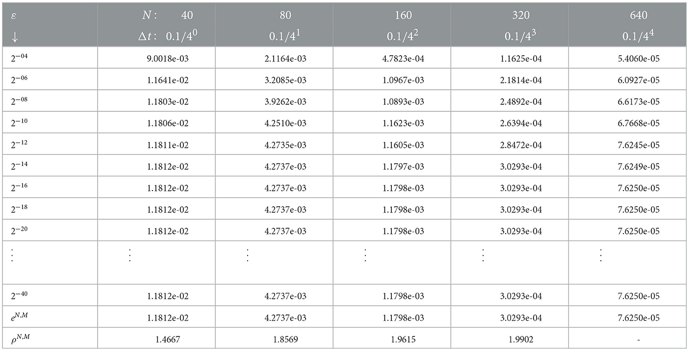
Table 1. Maximum absolute errors and uniform convergence rates of Example 1 at τ = ε/4.

TABLE 2

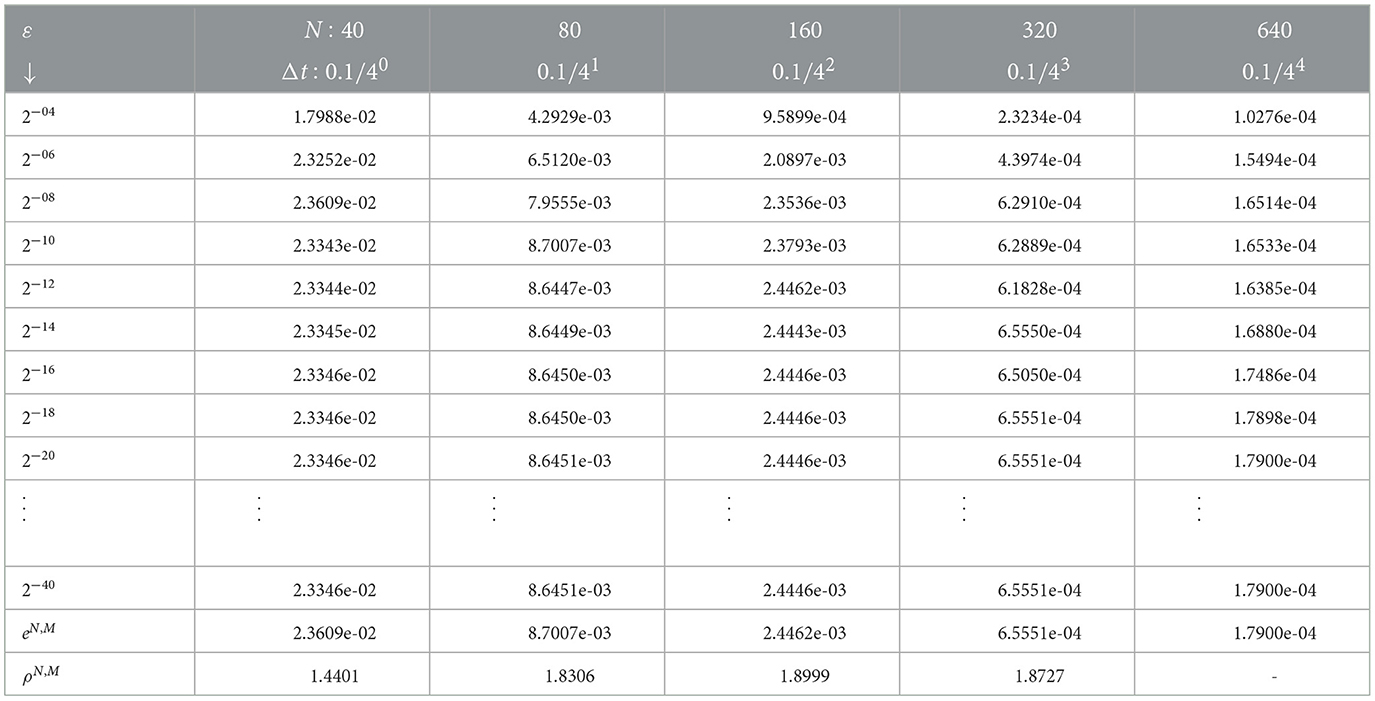
Table 2. Maximum absolute errors and uniform convergence rates of Example 2 at τ = ε/4.

TABLE 3

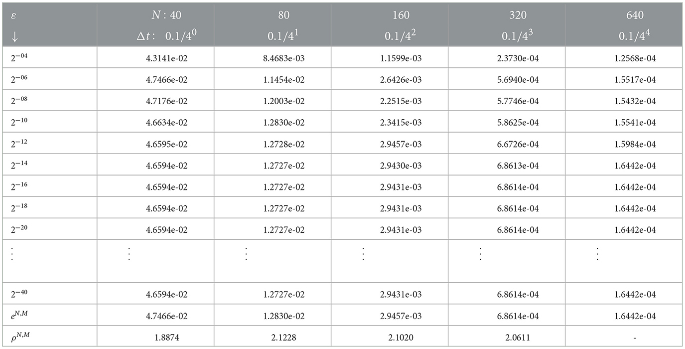
Table 3. Maximum absolute errors and uniform convergence rates of Example 3 at τ = ε/4.

In Figure 1, we observe the effect of the perturbation parameter in layer resolving for each example. Surface plots are simulated in Figures 2–4 for Examples 1–3, respectively. From each figure, we observe the effect of ε, that is, decreasing the values of ε decreases the width of the layers. The robustness of the developed scheme is illustrated by plotting log–log figures as given in Figure 5 for the considered examples.

FIGURE 1

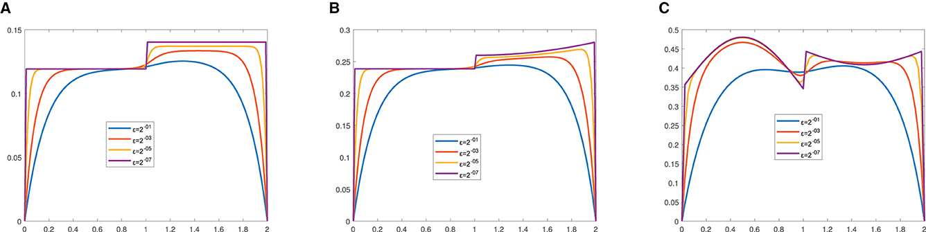
Figure 1. Effect of the perturbation parameter in resolving the boundary layers for (A) Example 1, (B) Example 2, and (C) Example 3 when τ = ε/4.

FIGURE 2

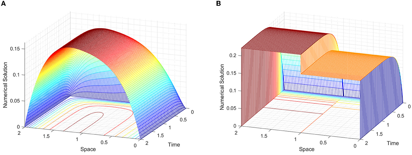
Figure 2. Surface plot simulations of Example 1, for various values of ε at τ = ε/4. (A) ε = 2⁰ and (B) ε = 2¹⁶.

FIGURE 3

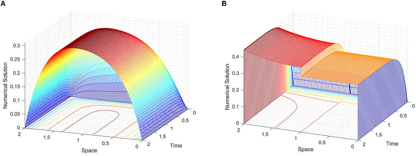
Figure 3. Surface plot simulations of Example 2, for various values of ε at τ = ε/4. (A) ε = 2⁰ and (B) ε = 2¹⁶.

FIGURE 4

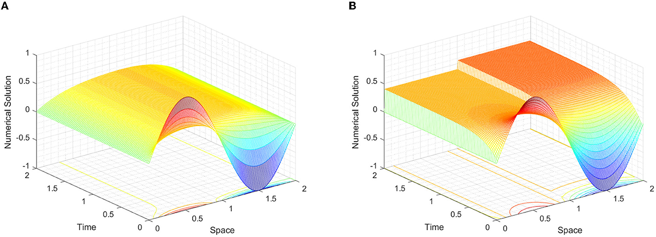
Figure 4. Surface plot simulations of Example 3, for various values of ε at τ = ε/4. (A) ε = 2⁰ and (B) ε = 2¹⁶.

FIGURE 5

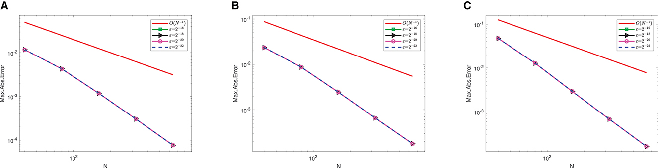
Figure 5. Log–log plots of N vs maximum absolute errors for (A) Example 1, (B) Example 2, and (C) Example 3.

5. Conclusion

In this study, we proposed and analyzed a fitted numerical method for a singularly perturbed differential equation involving spatial and temporal delays in the reaction term. The solution varies abruptly in the layers due to the presence of the perturbation parameter. The rapidly changing behavior of the layers and the effect of the delays cause difficulties to find the analytical solution. To solve the problem, we proposed a fitted numerical method. The method is obtained by using the implicit Euler method in the temporal variable and the nonstandard finite difference method in the spatial variable on uniform meshes. The effect of the temporal delay is handled by applying Taylor's series approximation and the spatial delay is handled by choosing a special mesh so that the delay term lies on the mesh point x_i = 1. We investigated and proved that the proposed method is stable and uniformly convergent. We considered and solved three model examples to test the validity and applicability of the proposed method. The solutions and accuracy of the results of the examples are shown in graphical and tabular forms. From the theoretical and numerical findings discussed in the article, we can conclude that the proposed numerical method is uniformly convergent of order one in time and of order two in space.

Data availability statement

The original contributions presented in the study are included in the article/supplementary material, further inquiries can be directed to the corresponding author.

Author contributions

GD initiated the plan of this study. AE proposed the numerical scheme and analysis of the results. MW and TD revised the procedures, analysis, and results of the study. All authors have equal contributions to the article and agreed on the submitted version.

Acknowledgments

The authors kindly thank the editor for handling the manuscript carefully and referees for their valuable contributions in modifying the original version of the manuscript.

Conflict of interest

The authors declare that the research was conducted in the absence of any commercial or financial relationships that could be construed as a potential conflict of interest.

Publisher's note

All claims expressed in this article are solely those of the authors and do not necessarily represent those of their affiliated organizations, or those of the publisher, the editors and the reviewers. Any product that may be evaluated in this article, or claim that may be made by its manufacturer, is not guaranteed or endorsed by the publisher.

References

1. Stépán G, Haller G. Quasiperiodic oscillations in robot dynamics. Nonlinear Dyn. (1995) 8:513–28. doi: 10.1007/BF00045711

PubMed Abstract | CrossRef Full Text | Google Scholar

2. Feng Z, Chicone C. A delay differential equation model for surface acoustic wave sensors. Sensors Actuators A Phys. (2003) 104:171–8. doi: 10.1016/S0924-4247(03)00052-9

CrossRef Full Text | Google Scholar

3. Epstein IR. Delay effects and differential delay equations in chemical kinetics. Int Reviews in Phy Chem. (1992) 11:135–60. doi: 10.1080/01442359209353268

CrossRef Full Text | Google Scholar

4. Barjau A, Gibiat V. Delayed models for simplified musical instruments. J Acoust Soc Am. (2003) 114:496–504. doi: 10.1121/1.1577558

PubMed Abstract | CrossRef Full Text | Google Scholar

5. Nagatani T, Nakanishi K. Delay effect on phase transitions in traffic dynamics. Phys Rev E. (1998) 57:6415. doi: 10.1103/PhysRevE.57.6415

PubMed Abstract | CrossRef Full Text | Google Scholar

6. Culshaw RV, Ruan S. A delay-differential equation model of HIV infection of CD4+ T-cells. Math Biosci. (2000) 165:27–39. doi: 10.1016/S0025-5564(00)00006-7

PubMed Abstract | CrossRef Full Text | Google Scholar

7. Gopalsamy K. Stability and Oscillations in Delay Differential Equations of Population Dynamics. Vol. 74. Springer Science & Business Media (2013). doi: 10.1007/978-94-015-7920-9

CrossRef Full Text | Google Scholar

8. Szydłowski M, Krawiec A. The Kaldor-Kalecki model of business cycle as a two-dimensional dynamical system. J Nonlinear Math Phy. (2001) 8:266–71. doi: 10.2991/jnmp.2001.8.s.46

CrossRef Full Text | Google Scholar

9. Mahendran R, Subburayan V. Fitted finite difference method for third order singularly perturbed delay differential equations of convection diffusion type. Int J Comput Methods. (2019) 16:1840007. doi: 10.1142/S0219876218400078

CrossRef Full Text | Google Scholar

10. Longtin A, Milton JG. Complex oscillations in the human pupil light reflex with mixed and delayed feedback. Math Biosci. (1988) 90:183–99. doi: 10.1016/0025-5564(88)90064-8

CrossRef Full Text | Google Scholar

11. Yang Y, Ouyang J, Ma L, Tseng RH, Chu CW. Electrical switching and bistability in organic/polymeric thin films and memory devices. Adv Funct Mater. (2006) 16:1001–14. doi: 10.1002/adfm.200500429

CrossRef Full Text | Google Scholar

12. Saksena VR, O'reilly J, Kokotovic PV. Singular perturbations and time-scale methods in control theory: survey 1976-1983. Automatica. (1984) 20:273–93. doi: 10.1016/0005-1098(84)90044-X

CrossRef Full Text | Google Scholar

13. Bocharov G, Romanyukha A. Numerical treatment of the parameter identification problem for delay-differential systems arising in immune response modelling. Appl Numer Math. (1994) 15:307–26. doi: 10.1016/0168-9274(94)00007-7

CrossRef Full Text | Google Scholar

14. Kot M. Elements of Mathematical Ecology. Cambridge: Cambridge University Press (2001).

Google Scholar

15. Schneider IAN. Spatio-Temporal Feedback Control of Partial Differential Equations. Berlin: Fereie University (2016). doi: 10.17169/refubium-5712

PubMed Abstract | CrossRef Full Text | Google Scholar

16. Batzel JJ, Kappel F. Time delay in physiological systems: analyzing and modeling its impact. Math Biosci. (2011) 234:61–74. doi: 10.1016/j.mbs.2011.08.006

PubMed Abstract | CrossRef Full Text | Google Scholar

17. Sharma KK, Rai P, Patidar KC. A review on singularly perturbed differential equations with turning points and interior layers. Appl Math Comput. (2013) 219:10575–609. doi: 10.1016/j.amc.2013.04.049

CrossRef Full Text | Google Scholar

18. Clavero C, Jorge JC. Another uniform convergence analysis technique of some numerical methods for parabolic singularly perturbed problems. Comput Math Appl. (2015) 70:222–35. doi: 10.1016/j.camwa.2015.04.006

PubMed Abstract | CrossRef Full Text | Google Scholar

19. Erdogan F, Cen Z. A uniformly almost second order convergent numerical method for singularly perturbed delay differential equations. J Comput Appl Math. (2018) 333:382–94. doi: 10.1016/j.cam.2017.11.017

CrossRef Full Text | Google Scholar

20. Alam MP, Kumar D, Khan A. Trigonometric quintic B-spline collocation method for singularly perturbed turning point boundary value problems. Int J Comput Math. (2021) 98:1029–48. doi: 10.1080/00207160.2020.1802016

CrossRef Full Text | Google Scholar

21. Gupta V, Kumar M, Kumar S. Higher order numerical approximation for time dependent singularly perturbed differential-difference convection-diffusion equations. Numer Methods Partial Diff Equat. (2018) 34:357–80. doi: 10.1002/num.22203

CrossRef Full Text | Google Scholar

22. Kehinde OO, Munyakazi JB, Appadu AR. A NSFD discretization of two-dimensional singularly perturbed semilinear convection-diffusion problems. Front Appl Math Stat. (2022) 8:861276. doi: 10.3389/fams.2022.861276

CrossRef Full Text | Google Scholar

23. Mbroh NA, Munyakazi JB. A fitted operator finite difference method of lines for singularly perturbed parabolic convection-diffusion problems. Math Comput Simulat. (2019) 165:156–71. doi: 10.1016/j.matcom.2019.03.007

CrossRef Full Text | Google Scholar

24. Ansari A, Bakr S, Shishkin G. A parameter-robust finite difference method for singularly perturbed delay parabolic partial differential equations. J Comput Appl Math. (2007) 205:552–66. doi: 10.1016/j.cam.2006.05.032

CrossRef Full Text | Google Scholar

25. Sahoo SK, Gupta V. Higher order robust numerical computation for singularly perturbed problem involving discontinuous convective and source term. Math Methods Appl Sci. (2022) 45:4876–98. doi: 10.1002/mma.8077

CrossRef Full Text | Google Scholar

26. Appadu AR, Tijani YO. 1D generalised burgers-huxley: proposed solutions revisited and numerical solution using FTCS and NSFD methods. Front Appl Math Stat. (2022) 7:773733. doi: 10.3389/fams.2021.773733

CrossRef Full Text | Google Scholar

27. Ejere AH, DuressaGF, Woldaregay MM, Dinka TG. An exponentially fitted numerical scheme via domain decomposition for solving singularly perturbed differential equations with large negative shift. J Math. (2022) 2022:1–13. doi: 10.1155/2022/7974134

CrossRef Full Text | Google Scholar

28. Kumari P, Kumar D. Parameter-uniform numerical treatment of singularly perturbed initial-boundary value problems with large delay. Appl Num Math. (2020) 163:412–29. doi: 10.1016/j.apnum.2020.02.021

CrossRef Full Text | Google Scholar

29. Bansal K, Sharma KK. Parameter-Robust numerical scheme for time-dependent singularly perturbed reaction-diffusion problem with large delay. Numer Funct Anal Optim. (2018) 39:127–54. doi: 10.1080/01630563.2016.1277742

CrossRef Full Text | Google Scholar

30. Ejere AH, Duressa GF, Woldaregay MM, Dinka TG. A uniformly convergent numerical scheme for solving singularly perturbed differential equations with large spatial delay. SN Appl Sci. (2022) 4:1–15. doi: 10.1007/s42452-022-05203-9

PubMed Abstract | CrossRef Full Text | Google Scholar

31. Alam MP, Khan A. A new numerical algorithm for time-dependent singularly perturbed differential-difference convection-diffusion equation arising in computational neuroscience. Comput Appl Math. (2022) 41:402. doi: 10.1007/s40314-022-02102-y

CrossRef Full Text | Google Scholar

32. Kadalbajoo MK, Gupta V. A brief survey on numerical methods for solving singularly perturbed problems. Appl Math Comput. (2010) 217:3641–16. doi: 10.1016/j.amc.2010.09.059

CrossRef Full Text | Google Scholar

33. Roos HG, Stynes M, Tobiska L. Robust Numerical Methods for Singularly Perturbed Differential Equations: Convection-Diffusion-Reaction and Flow Problems. Vol. 24. Springer Science & Business Media (2008). doi: 10.1007/978-3-540-34467-4

CrossRef Full Text | Google Scholar

34. Kellogg RB, Tsan A. Analysis of some difference approximations for a singular perturbation problem without turning points. Math Comput. (1978) 32:1025–39. doi: 10.1090/S0025-5718-1978-0483484-9

PubMed Abstract | CrossRef Full Text | Google Scholar

35. Clavero C, Gracia JL. On the uniform convergence of a finite difference scheme for time dependent singularly perturbed reaction-diffusion problems. Appl Math Computat. (2010) 216:1478–88. doi: 10.1016/j.amc.2010.02.050

CrossRef Full Text | Google Scholar

36. Ehrhardt M, Mickens RE. A nonstandard finite difference scheme for convection-diffusion equations having constant coefficients. Appl Math Comput. (2013) 219:6591–604. doi: 10.1016/j.amc.2012.12.068

CrossRef Full Text | Google Scholar

37. Woldaregay MM, Duressa GF. Uniformly convergent numerical method for singularly perturbed delay parabolic differential equations arising in computational neuroscience. Kragujevac J Math. (2022) 46:65–84. doi: 10.46793/KgJMat2201.065W

CrossRef Full Text | Google Scholar

38. Munyakazi JB, Patidar KC. A fitted numerical method for singularly perturbed parabolic reaction-diffusion problems. Comput Appl Math. (2013) 32:509–19. doi: 10.1007/s40314-013-0033-7

CrossRef Full Text | Google Scholar