Implementation of the banking dynamics model using a system of deterministic differential equations

Introduction: This study discusses modeling the interaction among components of a bank’s balance sheet, consisting of deposit, loan, and equity, as a useful tool for analyzing risk conditions arising from factors such as non-performing loans (NPSLs) and deposit withdrawals.

Methods: The model utilizes a deterministic differential equation system based on a modified logistic growth model.

Results: When applied to data of selected banks in Indonesia under certain assumptions, the model effectively describes the growth of their balance sheets.

Discussion: Our findings indicate that banks with higher core capital do not necessarily exhibit more stable equilibrium than those with lower core capital. Additionally, the equity equilibrium does not show a consistent pattern among banks with varying levels of core capital.

1 Introduction

Banks are important institutions for maintaining the stability of a nation’s economy. Their main function is to collect funds as deposits and redistribute them in the form of credit, commonly referred to as loans, often interchangeably. In carrying out these operational activities, banks profit from the difference between loan interest and deposit interest, taking risks into consideration. Increases in loans distributed by banks lead to higher profits, but the risk of loss from non-performing loans (NPLs), which are loans that fail to be paid back by borrowers, also increases. A high proportion of NPL reduces the amount of the bank’s assets, meaning that these assets, originally deposits held by the bank’s customers, cannot be withdrawn by them. This creates a solvency risk, where the bank’s assets become less valuable than its liabilities. If customers are unable to withdraw their own money, it can alert customers at other banks, prompting them to withdraw all their funds as a precaution. This phenomenon is called systemic risk, causing people to lose trust in banking, leading to a reluctance to deposit their funds. Consequently, those in need of investment funds may find it challenging to borrow from banks, resulting in slower economic growth.

When banks fail to assess risk properly and experience losses, customers who lose trust tend to withdraw their savings. This can result in liquidity risk, which can lead to banks going bankrupt. This loss of trust can quickly extend to customers of other banks. When too many banks go bankrupt, the economic stability of a nation is severely affected. For example, one of the causes of the 2008 global financial crisis was the distribution of high-risk housing loans in excessive amounts without adequate regulation. This distribution caused an increase in the average portion of non-performing loans (NPLs). When the value of housing loans fell, coupled with a large portion of NPLs, many banks incurred significant losses. In the USA, the bankruptcy of Lehman Brothers triggered a financial crisis and a loss of confidence, which subsequently led to a liquidity crisis. During the 2007–2008 economic crisis, 465 banks were declared bankrupt. When public confidence in the Rupiah currency fell in Indonesia, it led to massive withdrawals and contributed to the 1997–1998 Indonesian Monetary Crisis (1). In this incident, 16 Indonesian banks went bankrupt, triggering massive inflation that caused economic and political instability.

Binding policies are essential to ensure that banking activities operate smoothly within a nation. To establish the right policy, research and data analysis are necessary for modeling the dynamics of banking. One study that has been conducted involves the mathematical modeling of bank balance sheets, known as banking models. These banking models can be expressed using dynamic models that track changes in the values of bank balance sheet components over a specific period. Factors that affect the values of bank balance sheet components are represented as variables in a differential equation.

The use of a system of differential equations allows researchers to determine the growth of observed objects over extended periods and the conditions under which they reach equilibrium. The dynamic model presented in this study, structured as a system of differential equations, is based on the predator–prey model, which has applications in various fields, including banking, as demonstrated by Caravaggio and Sodini (2), Blyuss et al. (3), Fakhry et al. (4), McLean et al. (5), and Saini et al. (6). The development of the dynamic model for creating a banking framework is discussed in Sumarti et al. (7, 8) and Ansori et al. (9–13) as well as in Ansori (14), Atangana and Khan (15), Ananth et al. (16), and Aqsha (17). Previously, the bank balance sheet model consisted solely of deposits and loans. In Sumarti et al. (8), it was expanded to include additional components from the bank’s financial statements. Modifications to the model to incorporate interbank interactions were implemented by Ansori et al. (9, 10), with the introduction of additional operators by Atangana and Khan (15) and Ananth et al. (16). The application of a metaheuristic method to address model optimization problems was initially introduced by Ansori et al. (9). Utilizing the method outlined by Ansori et al. (11), researchers can assess the stability of the bank’s component equilibria and perform sensitivity analyses to predict banking health and extend the stability of the banking system. One advantage of employing a dynamic model is its modular nature, which facilitates the addition or removal of variables. For example, the incorporation of a stochastic component into the dynamic model for representing a bank’s balance sheet is explored by Ansori et al. (12). A similar dynamic model is applied by Ansori et al. (13) to simulate a banking network system and analyze macroprudential policy.

This study discusses a model for modeling the bank’s balance sheet and its implementation. As our new contribution to the existing research, real data from banks in Indonesia and the latest banking regulations in Indonesia that significantly improved the model are used. Using a metaheuristic optimization method, the model’s parameters can be obtained, which are then used to calculate each bank component’s equilibrium and stability. Selected parameter values are then changed to observe the change in equilibrium value and stability. The results from the model can suggest the bank balance’s trend and its sensitivity to some significant factors, which could predict the risks of liquidity and solvency of the bank. The model can be used by the regulator to analyze the impact of proposed regulations related to banks to maintain the stability of the banking and financial industries.

2 Methodology and data

2.1 Construction of model

Modeling bank balance sheets using a system of deterministic differential equations is presented in Ansori (14) and further expanded in Aqsha (17). Using real data from commercial banks, this study demonstrates the model’s implementation, as discussed in Aqsha (17), along with some modifications to better describe the bank’s reverse operations. The model uses a simplified bank balance sheet, which includes assets, liabilities, and equity, along with the following simplifications:

A. Assets consist of loans distributed by the bank, securities owned by the bank, reserves at the central bank, and liquid assets consisting of assets that are easily converted into cash. Liquid assets serve as the balance sheet balancer in this simplified version of the banking balance sheet.

B. Deposit made up the entire liabilities.

C. It is assumed that there is no interaction between banks.

The model predicts the value of bank components based on their changes in value over a specified time interval. The chosen components are deposits, loans, and equity. The equations for deposit and loan growth are assumed to follow a logistic model with the following descriptions:

• The deposit growth follows a logistic model that is influenced by deposit $D\left(t\right)$ and decreases when there is withdrawal $\omega D\left(t\right)$ with a value proportional to the deposit value.

• The loan growth follows a logistic model that is influenced by the value of loan $L\left(t\right)$ , liquid asset $A\left(t\right)$ , and reserve $R\left(t\right)$ . Loan values decrease when there is NPL $\eta L\left(t\right)$ or returned loan $\delta \left(1-n\right)L\left(t\right)$ .

• The equity growth is influenced by the equity value $E\left(t\right)$ and decreases by the portion of NPL.

Deposit, loan, and equity growths can be expressed by a system of differential equations as follows:

$\{\begin{array}{l}\frac{dD\left(t\right)}{dt}={\alpha }_{D}D\left(t\right)\left(1-\frac{D\left(t\right)}{K_D}\right)-\omega D\left(t\right),\hfill \\ \frac{\mathit{dL}\left(t\right)}{dt}={\alpha }_{L}L\left(t\right)A\left(t\right)\left(1-\frac{L\left(t\right)}{K_L}\right)-\eta L\left(t\right)-\delta \left(1-n\right)L\left(t\right),\hfill \\ \frac{dE\left(t\right)}{dt}={\alpha }_{P}P\left(t\right)-\eta L\left(t\right)\text{,}\hfill \end{array}\text{ (1)}$

$\begin{array}{ll}A\left(t\right)=D\left(t\right)+E\left(t\right)-L\left(t\right)-R^{\ast }\left(t\right)\text{.}& (2)\end{array}$

It is important to note that the bank’s reserve $R^{\ast }\left(t\right)$ regulated by the central bank gives no interest or return. The bank usually allocates its assets into financial securities, which is called a part of the secondary reserve that gives a return as the bank’s income. We define the financial securities, which are allocated from some portion of the deposit or $S\left(t\right)=c_{B}D\left(t\right)$ , so Equation 2 becomes

$\begin{array}{ll}A\left(t\right)=D\left(t\right)+E\left(t\right)-L\left(t\right)-R\left(t\right)-S\left(t\right)\text{.}& (3)\end{array}$

Bank profits are obtained from the loan interest, excluding NPL, the interest on liquid assets that are commonly loaned to other banks overnight, and the securities yield. Factors that cause profits to decrease are the savings interest rate excluding withdrawals, the equity yield, and the operational cost. The bank’s profit is expressed as follows:

$\begin{array}{l}P\left(t\right)=r_L\left(t\right)\left(1-n\right)L\left(t\right)+r_{A}A\left(t\right)-r_D\left(t\right)\left(1-w\right)\\ \mathrm{}D\left(t\right)-r_{E}E\left(t\right)+r_{S}S\left(t\right)-C\left(t\right)\end{array}\text{ (4)}$

The term $r_{S}S\left(t\right)$ , which is the return from the financial securities, is an addition to the original model (17). The bank’s operational cost is simplified using the linear model as stated in Equation 5.

$\begin{array}{ll}C\left(t\right)=c_{D}D\left(t\right)+c_{L}L\left(t\right)& (5)\end{array}$

The growth rates of deposits and loans depend on the interest rate based on the Monti-Klein model. The growth rate of deposits is also influenced by the condition of the equity. When the equity value declines, the deposit growth rate will also decline. Parameter formulas for deposit and loan growth rates are stated in the following equations.

$\begin{array}{ll}{\alpha }_D=\frac{m_D{r}_D\left(t\right)+b_D}{1+exp\left(-{\nu }_{D}E\left(t\right)\right)}\text{,}& (6)\end{array}$

$\begin{array}{ll}{\alpha }_L=-m_L{r}_L\left(t\right)+b_L& (7)\end{array}$

As in Ansori (14) and Aqsha (17), the bank reserve $R\left(t\right)$ used in this model consists of the primary reserve, a portion of the deposit, and the Loan to Deposit (LDR) Reserve. The central bank also requires the bank to keep the ratio of its LDR far away from a potentially high risk, in which the ratio is below or above the regulated interval value. As a control tool, an additional penalty amount that conditionally depends on the LDR ratio should be imposed on the bank’s reserve value. Equation 8 below expresses parameters utilized to model reserve value $R\left(t\right)$ . In the right-hand side of Equation 8, the first term is the primary reserve, and the second one is the additional LDR reserve.

$R\left(t\right)=\left({\rho }_P+{\rho }_S\right)D\left(t\right)+R_{LDR}\left(t\right)$

$R_{LDR\text{ (8)}}\left(t\right)=\{\begin{array}{ll}{\gamma }_{\mathit{lb}}\left({\lambda }_{\mathit{lb}}D\left(t\right)-L\left(t\right)\right)\hfill & ,\frac{S\left(t\right)+L\left(t\right)}{D\left(t\right)}<{\lambda }_{\mathit{lb}},\hfill \\ 0\hfill & ,{\lambda }_{\mathit{lb}}\le \frac{S\left(t\right)+L\left(t\right)}{D\left(t\right)}<{\lambda }_{ub},\hfill \\ {\gamma }_{ub}\left(L\left(t\right)-{\lambda }_{ub}D\left(t\right)\right)\hfill & ,\frac{S\left(t\right)+L\left(t\right)}{D\left(t\right)}\ge {\lambda }_{ub}\text{.}\hfill \end{array}$

The conditions in Equation 8 are originally only the loan-to-deposit ratio. Now, we put the securities variable into the ratio, which is required by the new regulation in Bank Indonesia (18–23).

The central bank can exempt a bank from paying the penalty on the third condition of the second term of Equation 8, where the ratio is higher than a regulated value ${\lambda }_{ub}\text{,}$ if the bank is considered very healthy. Note that the higher the amount of loan and securities, the larger the potential profit for the bank from their returns. If the bank has capital (or equity) satisfying a certain minimum ratio to the risk-weighted assets, and even if this ratio is higher than a threshold above the minimum requirement, the bank does not need to pay the penalty. The ratio formula is as follows.

$\begin{array}{ll}\frac{E\left(t\right)}{L\left(t\right)}\ge {\kappa }_1>{\kappa }_0\text{,}& (9)\end{array}$

where ${\kappa }_0$ is the minimum requirement value, and ${\kappa }_1$ is the threshold for exemption from the penalty of condition 3 in Equation 8.

Using Equation 8, Equation 3 can be rewritten as follows

$\begin{array}{ll}A\left(t\right)={\alpha }_{\mathit{AD}}D\left(t\right)+E\left(t\right)-{\alpha }_{AL}L\left(t\right)\text{,}& (10)\end{array}$

where

${\alpha }_{\mathit{AD}}=1-c_B-\{\begin{array}{ll}{\rho }_P+{\rho }_S+{\gamma }_{\mathit{lb}}{\lambda }_{\mathit{lb}}\hfill & ,\frac{S\left(t\right)+L\left(t\right)}{D\left(t\right)}<{\lambda }_{\mathit{lb}},\hfill \\ {\rho }_P+{\rho }_S-{\gamma }_{ub}{\lambda }_{ub}\hfill & ,\frac{S\left(t\right)+L\left(t\right)}{D\left(t\right)}>{\lambda }_{ub},\hfill \\ {\rho }_P+{\rho }_S\hfill & ,{\lambda }_{\mathit{lb}}\le \frac{S\left(t\right)+L\left(t\right)}{D\left(t\right)}\le {\lambda }_{ub}\text{.}\hfill \end{array}\text{ (11)}$

${\alpha }_{AL\text{ (12)}}=1+\{\begin{array}{ll}-{\gamma }_{\mathit{lb}}\hfill & ,\frac{S\left(t\right)+L\left(t\right)}{D\left(t\right)}<{\lambda }_{\mathit{lb}},\hfill \\ {\gamma }_{ub}\hfill & ,\frac{S\left(t\right)+L\left(t\right)}{D\left(t\right)}>{\lambda }_{ub},\hfill \\ 0\hfill & ,{\lambda }_{\mathit{lb}}\le \frac{S\left(t\right)+L\left(t\right)}{D\left(t\right)}\le {\lambda }_{ub}\text{.}\hfill \end{array}$

One of the advantages of this model is the ease of simplifying the bank balance sheet, and the parameters contained in the model can be easily changed, added, or reduced if the real situation requires it. Other approaches of the model stated in Equations 1–11 are defined stochastically and using the difference equations system recommended by Ansori (14) and Sumarti and Ansori (24).

Equation 1 shows the connection for each main component growth. Through ${\alpha }_{\mathit{AD}}$ , the equity value affects deposit growth, which decreases when equity value decreases. The value of deposits and equity affected the liquid assets that determine the loan growth. Through the bank’s operating profit, the value of deposits and loans affects equity growth.

The description of all variables is stated in Tables 1–3. Variable descriptions related to the Macroprudential Intermediation Ratio (Rasio Intermediasi Makroprudensial/RIM), which is a regulation in Indonesia regarding reserve value, are stated in Table 4. Parameters $\omega$ and $w$ have the same value and can be considered as the same parameter even though they have different dimensions. The same assumption is applied to variables $\eta$ and $n$ .

Table 1

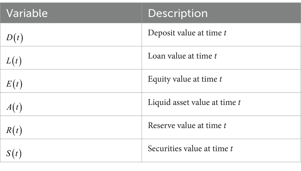
Table 1. Bank balance sheet component variables.

Table 2

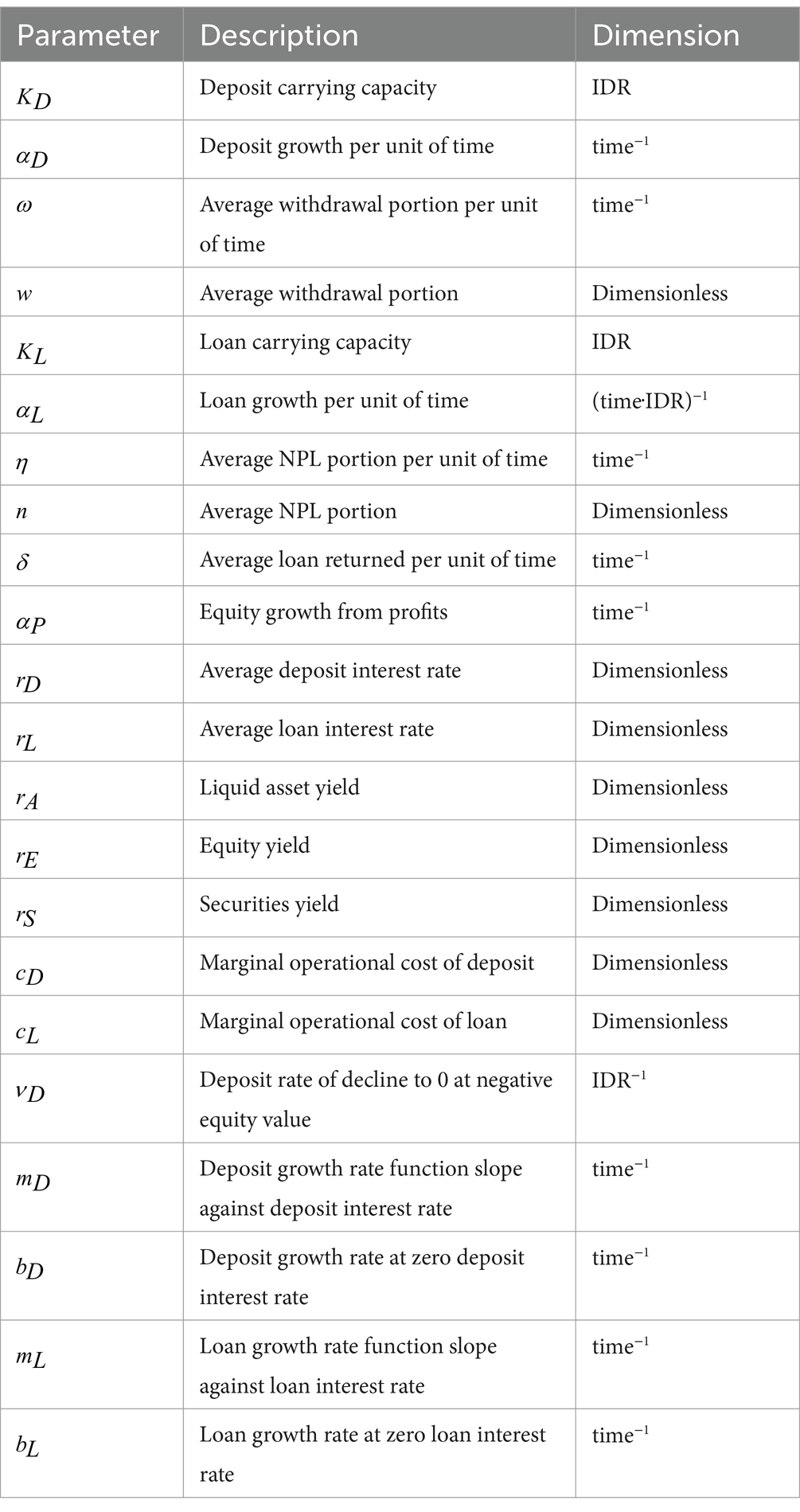
Table 2. Description and dimension of banking model parameters.

Table 3

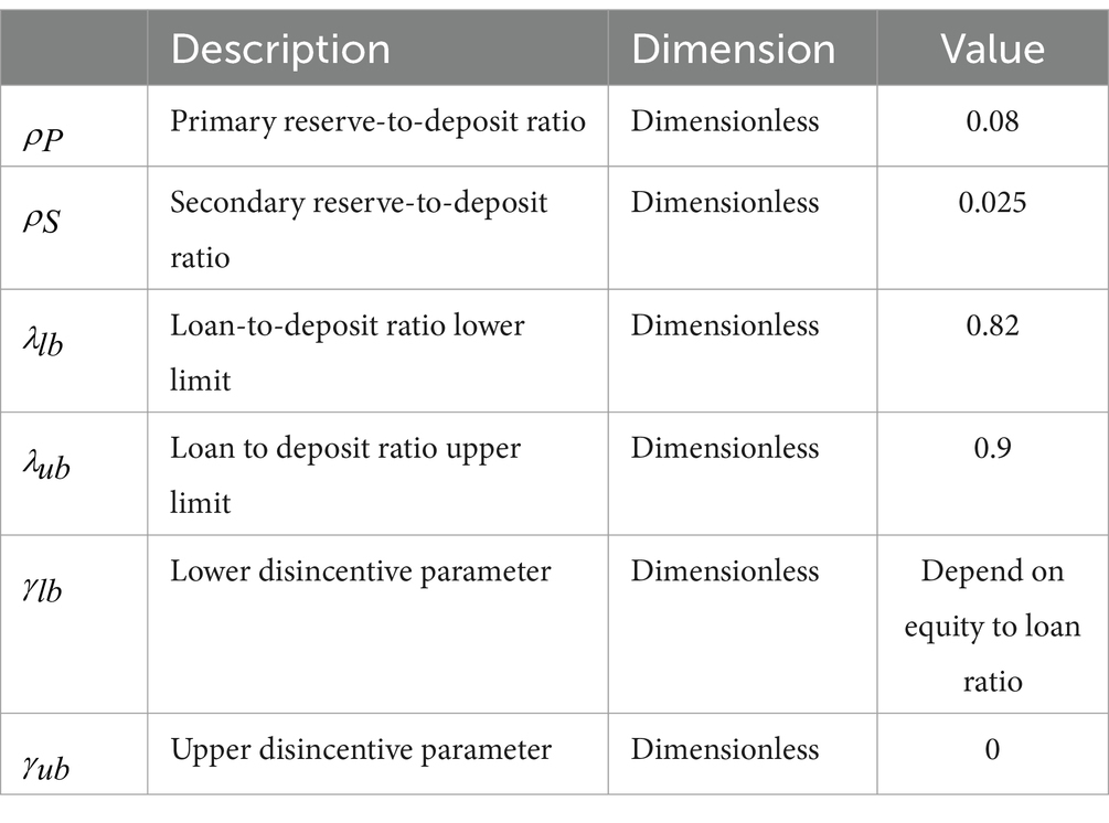
Table 3. Description and dimension of RIM parameters.

Table 4

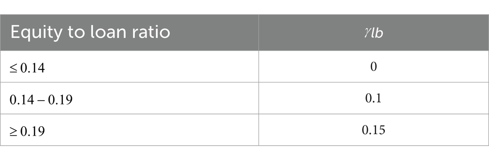
Table 4. Lower disincentive parameter value.

2.2 Mathematical methods of root finding and approximation

Due to interdependence among variables and quite a large number of parameters being observed, numerical methods for the equilibrium analysis and the estimation of parameters are inevitable. Define a vector $X$ containing variables $D,L$ , and $E$ , and $Y$ containing parameters in Table 2. Equation 1 can be rewritten as follows:

$\begin{array}{ll}\frac{dX}{dt}=F\left(t;X,Y\right)\text{,}& (13)\end{array}$

where $F$ is a non-linear equation in ${\Re }^3$ . The equilibrium points of system (Equation 13) are defined by finding $X$ such that $F\left(t;X,Y\right)=0$ . Due to interdependence among variables, analytics solutions are impossible to obtain. As explained in Nocedal and Wright (25) or Burden and Faires (26), the Broyden method, a quasi-Newton technique for locating the roots of a system of non-linear equations, is utilized. The Jacobian matrix (or its inverse) is approximated using the following iterative technique. Let $X_n$ and $G\left(X_n\right)$ respectively be the values of $X$ and $F$ at the $n$th-iteration.

$X_{n+1}=X_n+B_{n}G\left(X_n\right),n=0,1,\dots ,k_{\text{max}}\text{,}$

where $B_n$ approximates the inverse Jacobian matrix derived from Equation 11.

$B_{n+1}=B_n+\frac{\left(p_n-B_n{f}_n\right)}{p_n^T{f}_n}{p}_n^T\text{,}$

which $p_n=X_{n+1}-X_n$ , and $f_n=G\left(X_{n+1}\right)-G\left(X_n\right)$ .

Based on observations on data over a long time period, the interest rates of deposits and loans have fluctuated behavior and seem to follow a sinusoidal function. One of the series containing sinusoidal functions is the Fourier series. Define $N_i$ the number of terms being used for interest rate- $i$ , where $i=1$ for deposit and $i=2$ for loan. $T_i$ are the time lengths of data being used. In this research, we define for all $i,N_i=2,T_i=10$ years. The formula for the Fourier series is the following.

$r_i\left(t\right)=p_0^i+{\displaystyle \sum }_{n=1}^{N_i}{p}_n^{i}cos\left(\frac{2n\pi t}{T_i}\right)+q_n^{i}sin\left(\frac{2n\pi t}{T_i}\right)\text{.}$

We find parameters $p_n^i$ and $q_n^i$ that suit the data using the curve fitting method. In the equilibrium analysis, the interest rate values need to be constant, so we use the average value of the interest rate in the observed time period.

A different approach is employed in the estimation of $Y$ , due to quite a large number of parameters being estimated. We use an optimization approach that applies metaheuristic numerical method called Spiral Optimization Algorithm (SOA), which is a population-based algorithm that explores the search space using spiral trajectories.

Let ${\overline{X}}_t^i$ be the real data of a particular bank at time $t$ , ${\overline{X}}_t^1,{\overline{X}}_t^2\text{,}$ and ${\overline{X}}_t^3$ are deposit, loan, and equity data. We define the optimization problem, which is derived from the Mean Absolute Percentage Error (MAPE).

$\begin{array}{ll}\underset{Y}{min}\frac{1}{3}{\displaystyle \sum }_1^3\left(\frac{1}{N}{\displaystyle \sum }_{t=1}^N\frac{\left({\overline{X}}_t^i-X_t^i\right)}{{\overline{X}}_t^i}\right)\text{.}& (14)\end{array}$

In the SOA method, first, we define the initial search points $Y_i,i=1,2,\dots ,M$ , where $M$ is a previously defined number for the size of the population. We generate these points using the Sobol Sequence that gives uniform partitions of each point. Set the center point $Y_C$ of the centroid of the initial population. At each iteration, update the search points using a spiral trajectory as follows.

$\begin{array}{ll}{Y}_{n+1}=S_k\left(r,\theta \right)Y_n-\left(S_k\left(r,\theta \right)-I_k\right)Y_C\text{,}& (15)\end{array}$

where $r$ is the convergence rate, $0<r<1$ , and $\theta$ is the rotation angle, $0<\theta <2\pi$ . Matrix $I_k$ in Equation (15) is an $k\times k$ identity matrix, and $S_n\left(r,\theta \right)=r{R}^{\left(k\right)}\left({\theta }_{12},{\theta }_{13},\dots ,{\theta }_{k-1},{\theta }_k\right)$ with $R^{\left(k\right)}\left({\theta }_{12},{\theta }_{13},\dots ,{\theta }_{k-1},{\theta }_k\right)$ is the multiplication among all rotation matrices $R_{ij}^{\left(k\right)}\left({\theta }_{ij}\right)$ for all $i\ne j,1\le i,j\le k\text{.}$ We commonly have constant rotation angle $\theta ={\theta }_{ij}$ for all $i\ne j$ . A detailed algorithm of SOA can be found in Tamura and Yasuda (27) and Sidarto et al. (28).

The obtained value of the MAPE formula in Equation 14 is set as the measure of prediction accuracy for the estimation results. If the value is less than 10%, it is considered excellent forecasting accuracy. If it is between 10% and 20%, it is considered a good forecasting accuracy. We ran the algorithm and adjusted some algorithm parameters, such as $r$ and $\theta$ , so we obtained at least the good one.

2.3 Data implementation

In this study, data were obtained from the financial statements of banks in Indonesia, which are classified based on bank groups based on their core capital, which is called KBMI (Kelompok Bank Berdasarkan Modal Inti). Commercial banks are classified into four groups: KBMI 1 is banks with core capital of less than IDR 6 trillion; KBMI 2 is banks with core capital between IDR 6 trillion and IDR 14 trillion; KBMI 3 is banks with core capital between IDR 14 trillion and IDR 70 trillion; and KBMI 4 is banks with core capital of more than IDR 70 trillion.

Real data banks are selected from each KBMI; a private bank, Bank Victoria (KBMI 1); a regional development bank, BPD East Java (KBMI 2); a private bank, Bank Mega (KBMI 3); and a state-owned bank, Bank Rakyat Indonesia (KBMI 4). The selection of banks being considered is only one of each KBMI because we show the implementation of the system for the observation of individual banks.

The data provided by financial statements is presented in ${10}^6$ IDR. This value is then divided by a chosen number to facilitate optimization. Each data point from KBMI 1 data is divided by ${10}^7$ , KBMI 2 and KBMI 3 data is divided by ${10}^8$ , and KBMI 4 data is divided by ${10}^9$ . The relevant regulations from the central bank for determining the portion of bank reserve are taken from Bank Indonesia (18, 19, 21–23, 29).

The source of bank balance sheet component data was obtained from each bank’s quarterly financial reports with a time period between January 2014 and December 2023. Actual deposit and loan interest rates are obtained from Bank Indonesia and the Financial Services Authority (Otoritas Jasa Keuangan/OJK). Data on deposit interest rates was determined based on the type of bank, and data on loan interest rates is taken from each bank’s financial report.

Before solving the system of Equation 1 using the 4^th-order Runge–Kutta method, or specifically ODE45 in MATLAB, we estimated the values of all parameters by applying the SOA method to the optimization problem (Equation 14). The obtained parameter values were then used to determine the equilibrium of the model. In determining the equilibrium, the operational costs were approximated by a linear function according to Equation 5, and the deposit and loan interest rates were taken from the average value in one period. The equilibrium $D^{\ast },L^{\ast },E^{\ast }$ were obtained based on the following equation:

$\{\begin{array}{l}0={\alpha }_D{D}^{\ast }\left(1-\frac{D^{\ast }}{K_D}\right)-\omega D\left(t\right),\hfill \\ \begin{array}{l}0={\alpha }_L{L}^{\ast }\left({\alpha }_{\mathit{AD}}{D}^{\ast }+E^{\ast }-{\alpha }_{AL}{L}^{\ast }\right)\\ \mathrm{}\left(1-\frac{L^{\ast }}{K_L}\right)-\left(\eta +\delta \left(1-n\right)\right)L^{\ast },\end{array}\hfill \\ 0={\alpha }_P{P}^{\ast }-\eta L\left(t\right)\text{,}\hfill \end{array}\text{ (16)}$

where $P^{\ast }$ is the profit value when the deposit, loan, and equity are in the equilibrium points. This system of equations is difficult to solve analytically because it contains exponential and polynomial components, so we use numerical methods described in Section 2.2. There are a few things to consider in finding solutions:

• In the Broyden method, a fairly good guess of the starting point is needed so that the solution can converge. The guess value can be obtained by substituting $D^{\ast }$ to create a graph of the $L^{\ast }$ value against $E^{\ast }$ based on Equation 16, so that two curves are obtained. The intersection of the two curves indicates the values of $L^{\ast }$ and $E^{\ast }$ , which can be substituted to obtain the $D^{\ast }$value.

• Parameter values of ${\alpha }_{\mathit{AD}}$ and ${\alpha }_{AL}$in Equations 11, 12 have 9 different variations due to

Three conditions of the values of the mandatory minimum capital-loan ratio and the higher threshold as in Equation 9, where the ratio can be less than ${\kappa }_0$ , between ${\kappa }_0$ and ${\kappa }_1$ , and larger than ${\kappa }_1$ .

Three conditions of the values of the deposit-to-loan ratio with respect to their LDR ratio in Equation 8.

• In the calculation, values of ${\alpha }_{\mathit{AD}}$ and ${\alpha }_{AL}$ are set according to certain conditions. When the obtained solution does not meet the conditions used to obtain ${\alpha }_{\mathit{AD}}$ and ${\alpha }_{AL}$ , then the solution is discarded.

The stability analysis of obtained equilibrium points is carried out using the Routh-Hurwitz stability criteria. These point values are also used as an initial value in performing sensitivity analysis, which is performed by changing a parameter value and recomputing the equilibrium stability analysis based on the new parameter value. This study uses $\eta$ and $\omega$ as the sensitivity analysis parameters because these parameters are significant factors of the liquidity and solvency risks.

The steps of sensitivity analysis are as follows:

1. Start by establishing equilibrium at a specific value of either $\eta$ or $\omega$ .

2. In the first iteration, the parameters $\eta$ or $\omega$ are obtained from the SOA results.

3. Parameter values are added or subtracted from the preceding value to change the value of $\eta$ or $\omega$ .

4. With the new parameters $\eta$ or $\omega$ , the equilibrium is determined by the Broyden method with an initial guess from the previous iteration equilibrium.

5. The stability of the new equilibrium is determined by the Routh-Hurwitz stability criterion.

6. The process is repeated until the parameter value of $\eta$ or $\omega$ reaches the upper limit (maximum 1) and lower limit (minimum 0) that have been set.

7. An equilibrium graph is made against the parameter value by including stability indicators.

3 Results and discussion

In this section, we show the solutions to the system in Equations 1–12 for appointed banks, the equilibrium points of the system, and the sensitivity analysis using the NPL factor $\eta$ and the withdrawal factor $\omega \text{.}$ Figure 1 shows the value of each component in IDR, as stated in the balance sheet. The parameter optimization using SOA results in an MAPE value for each component from each bank, as stated in Table 5. See Appendix A for the obtained parameter values. Simulation for the bank’s components value fitness is indicated with the average MAPE value from each component, with the average MAPE value attributed to each bank below 10%, indicating a good fit for simulation.

Figure 1

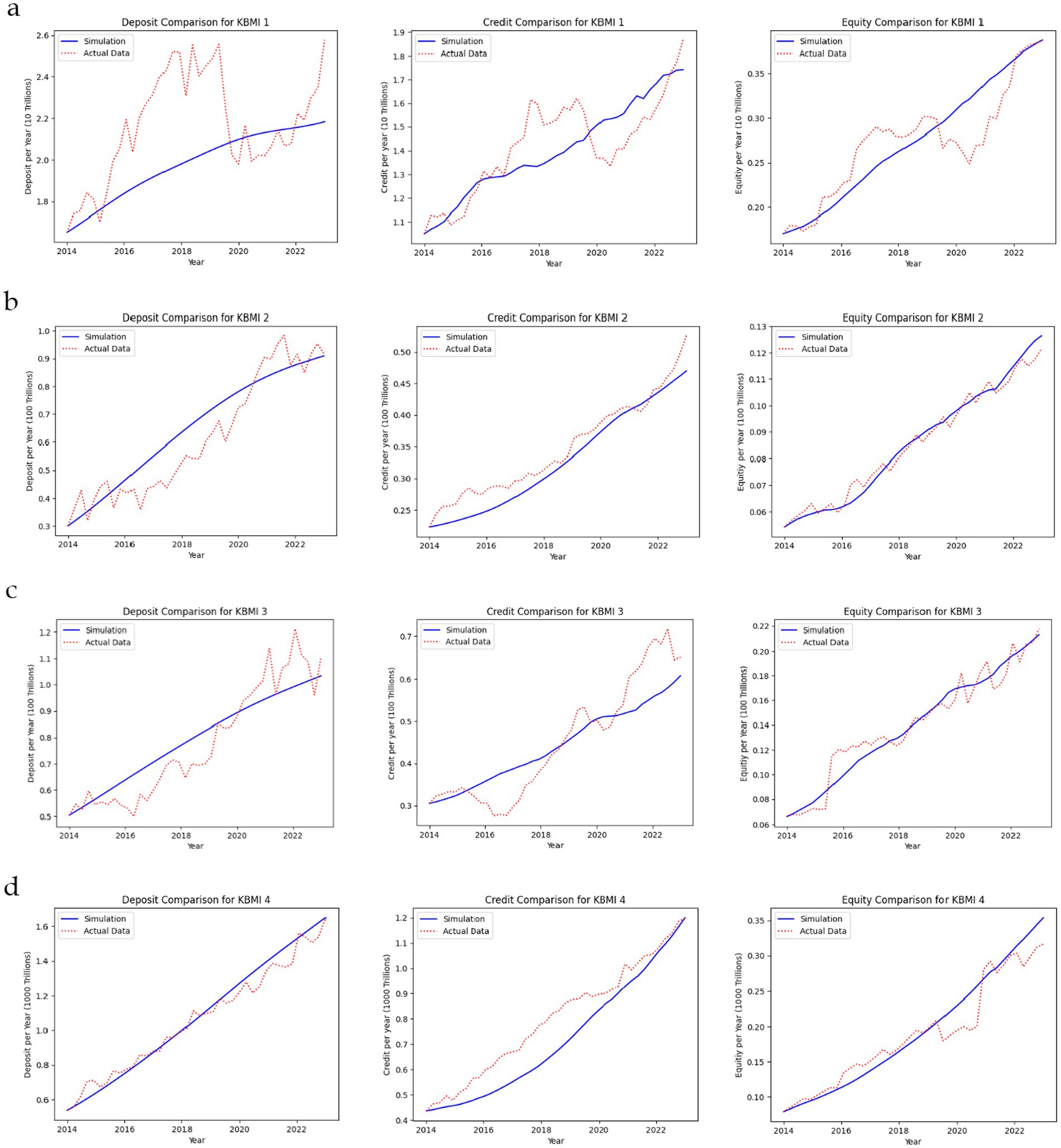
Figure 1. Simulation of bank’s components value. (a) Bank Victoria (KBMI 1). (b) BPD East Java (KBMI 2). (c) Bank Mega (KBMI 3). (d) BRI (KBMI 4).

Table 5

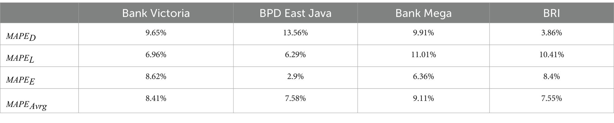
Table 5. MAPE values for each bank.

Figure 1 and Table 5 show the following:

• In the case of Bank Victoria, the model cannot capture big changes in value. While some parameter values can make the model adapt to small changes, the model is still based on the exponential growth model, which is better suited to observing changes in the trend’s values. As the average MAPE is used as the objective function, even though the deposit fit is not good, this is still considered the best fit by the spiral optimization algorithm, and the average MAPE value is less than 10%.

• The average MAPE value for BPD East Java and BRI are better than that of Bank Victoria and Bank Mega. These results can be attributed to the type of banks. Bank Victoria and Bank Mega are private banks, while BPD East Java and BRI are state-owned. More stable data leads to a better fit, and from the data chosen for this analysis, the state-owned banks are more stable than the private banks. This stability may result from an economically stable region in the case of BPD East Java or from the large core capital held by BRI. Further studies are required to compare the stability of state-owned banks with privately owned banks.

• Based on the original data in Figure 2, the deposit values of all banks are always larger than the loan values. However, later, in Table 6, the loan equilibrium points of Bank Victoria and BRI overshoot the deposit equilibrium points. The position of deposit and loan equilibrium points of BPD East Java are almost the same. The equilibrium points’ position for Bank Mega is almost the same as their initial solution.

Figure 2

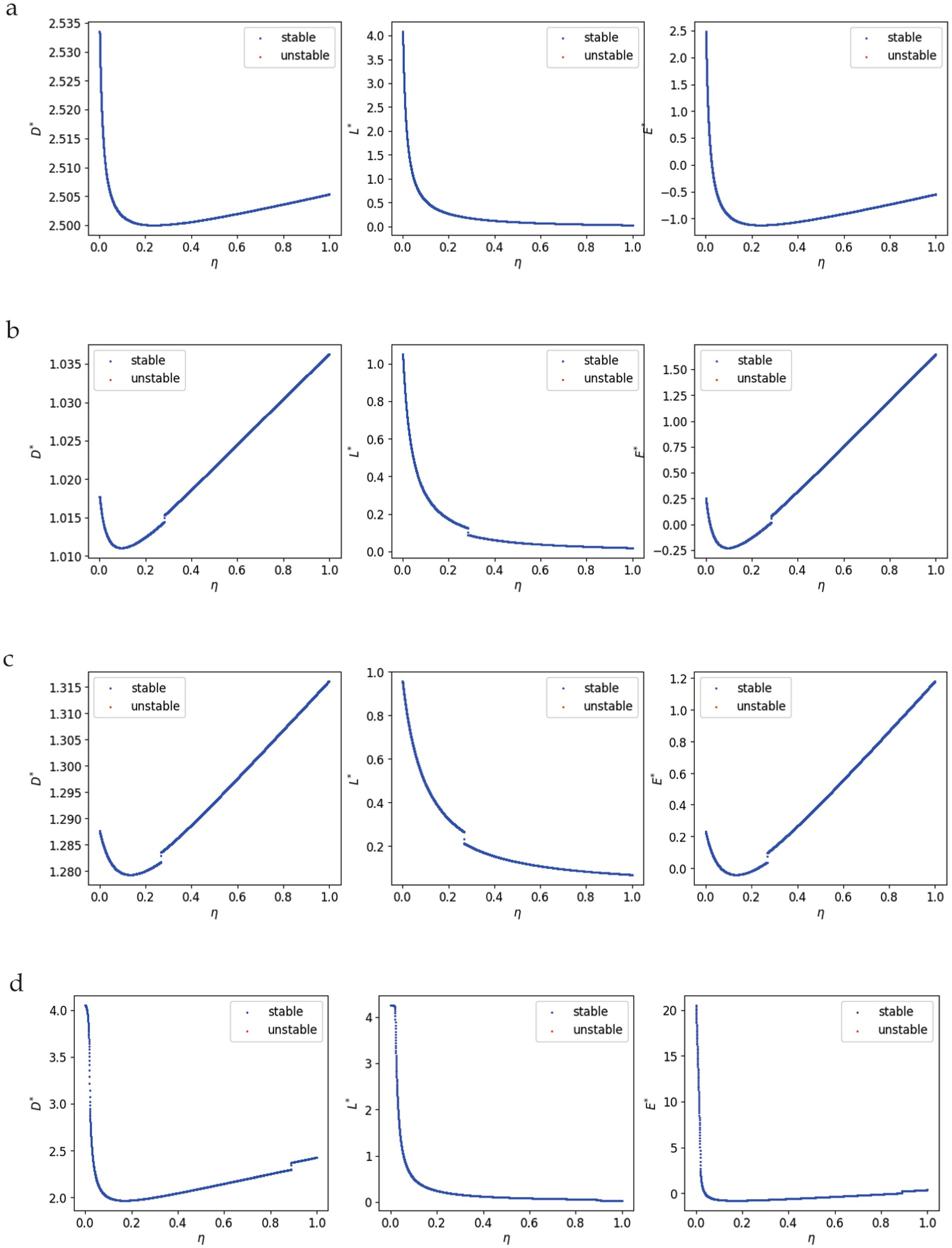
Figure 2. Sensitivity analysis for 𝜂 variation. (a) Bank Victoria (KBMI 1). (b) BPD East Java (KBMI 2). (c) Bank Mega (KBMI 3). (d) BRI (KBMI 4).

Table 6

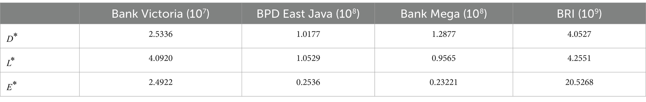
Table 6. Banks equilibrium points.

From the system, we identified more than one equilibrium point. Here, we only consider the equilibrium point to be positive and stable, as shown in Table 6. In the sensitivity analysis, the results are categorized as stable equilibrium or unstable equilibrium. A stable equilibrium indicates that the bank’s component value is almost certain to reach the equilibrium value. An unstable equilibrium has a lower probability of reaching the equilibrium value, or the solution could blow up to infinity or fall to minus infinity, impacting the bank’s ability to operate normally. Banks that have at least one component with a stable negative equilibrium value have a higher likelihood of going bankrupt than those that have at least one component with an unstable negative equilibrium value.

The results of the sensitivity analysis of the NPL value to equilibrium points in Figure 2 show that the obtained equilibrium points are all in blue color. It means that they are all stable. The behavior of the equilibrium points for each component is described in the following paragraphs.

When the NPL value rises, the loan equilibrium depicted in the center graph of all banks in Figure 2 declines rapidly. When the loan equilibrium reaches zero, the pace of decline slows. Long-term high non-performing loan (NPL) values make it more likely for banks to lose their loan balances.

The left and right graphs of all banks in Figure 2 show very similar behaviors for the deposit and equity equilibrium points, respectively. For low NPL levels, they are declining, but then they start to rise again. According to Equation 8, the growth rate of the deposit ${\alpha }_D$ is influenced by the equity value, and it appears that the behavior of the deposit equilibrium mimics that of the equity equilibrium.

The equity equilibrium decreases until a certain $\eta$ then increases, which is the reflection of the behavior of the equity value. According to Equation 1, the equity growth rate depends on the difference between the portion of profit value and the portion of loan value. For the low value of NPL, the increase in profit cannot withstand the increase of the loan, so the equity decreases. For a large value of NPL, even though the profits decrease, the value of the loan is much smaller, so the equity will increase.

The equity equilibrium for high NPL value is negative for Bank Victoria, suggesting that if the manager does nothing to control the non-performing loan, there may be an insolvency condition. The situation is different with BPD East Java, where the negative value is only for certain values of NPL.

As the NPL value rises, so do the equity equilibriums of Bank Mega and BPD East Java. The rising NPL does not appear to be an issue. The behavior of the original related solution in Figure 2 is consistent with the original equilibrium points of the deposit for BPD East Java and Bank Mega in Table 6, where they are almost identical or larger than those of the loan. It indicates that deposit growth is outpacing loan growth. Strong deposit growth influences the rise in liquid assets, which ultimately leads to a profit and an increase in quantity. It could be the cause of the NPL growth’s seeming lack of issues for both banks.

However, in this sensitivity analysis, the values of other parameters remain constant, as shown in Appendices A, B. Their values cannot remain constant with these outcomes, particularly for the parameters of deposit and equity growth, if the situation is changing. There may be a psychological impact of putting the banks in serious danger of going bankrupt, which causes customers and bank owners to lose faith in the bank’s management in the handling of their funds.

Now, we discuss the results of the sensitivity analysis for the withdrawal parameter $\omega$ . With the exception of BRI, Figure 3 illustrates that if the bank’s withdrawal parameter is more than 50%, even than 40% for BPD East Java, the bank will become bankrupt since the equilibrium points of equity, loans, and deposits are zero. Because loan value is reliant on reserves and liquid assets, it will go to zero as deposit value does. Zero loan value results in zero equity value since the bank’s profit is linked to loans. However, the unstable status, highlighted in red in Figure 3, for some equilibrium points means the values could just not be permanent. They can increase to positive values or decrease to negative values for equity values.

Figure 3

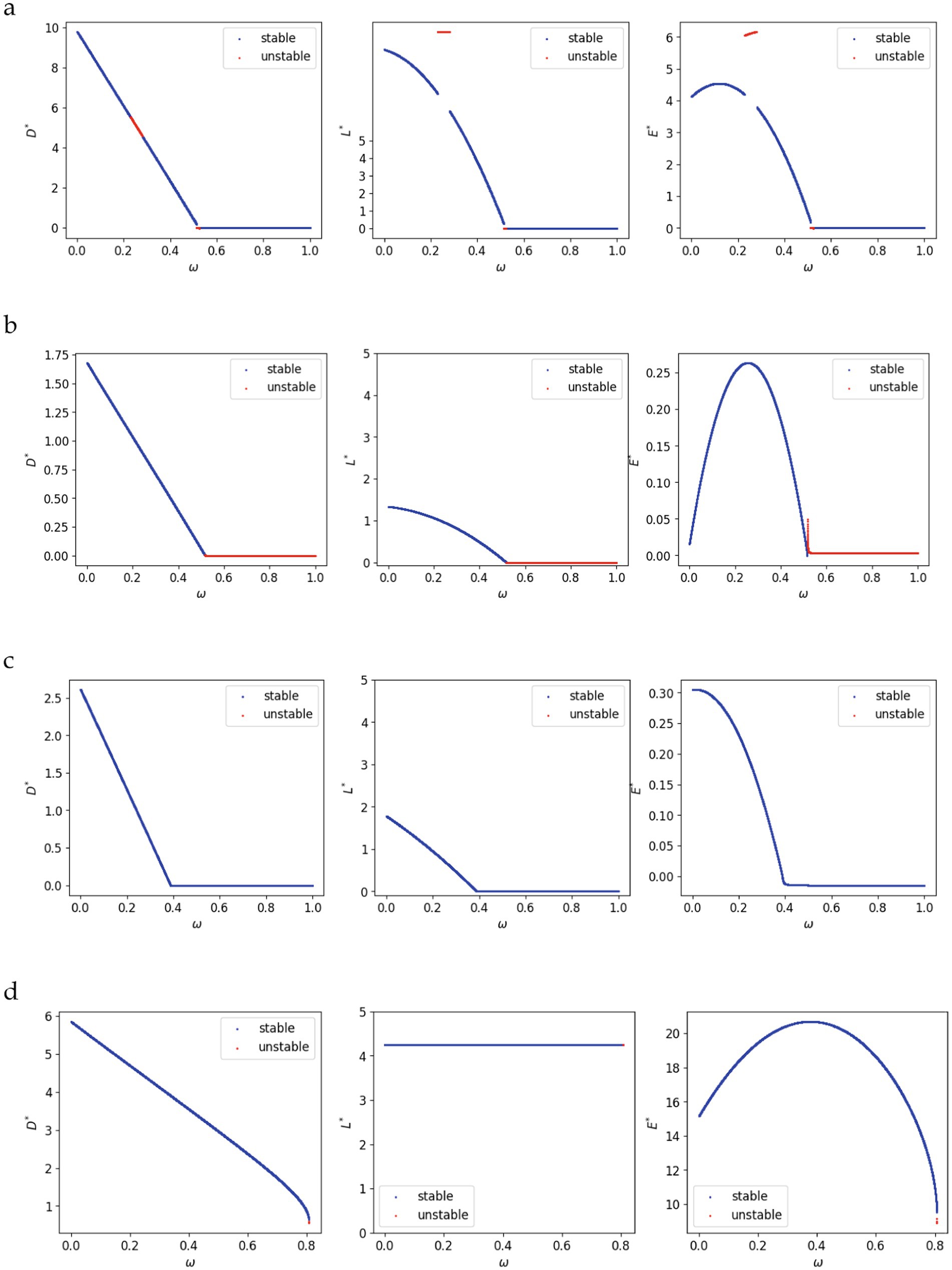
Figure 3. Sensitivity analysis for 𝜔 variation. (a) Bank Victoria (KBMI 1). (b) BPD East Java (KBMI 2). (c) Bank Mega (KBMI 3). (d) BRI (KBMI 4).

The deposit equilibrium in Figure 3d for BRI decreases but does not approach zero if the withdrawal parameter value increases. The loan equilibrium remains constant at its carrying capacity $K_L$ for all values of the withdrawal parameter $\omega$ . It appears that the strong growth of loans has already separated from the growth of deposits. Conversely, for small values of $\omega$ up to around 40%, deposit growth has little effect on the equity equilibrium; after that, a high value of $\omega$ causes it to deteriorate.

Based on the data used, the conditions of each bank determine the sensitivity analysis of parameter $\omega$ . It is not necessarily the case that banks in a higher KBMI category have a stable equilibrium than those in a lower KBMI. Furthermore, when banks from different KBMI groups are analyzed, no specific pattern has emerged from the movement of equity equilibrium. Therefore, more investigation is required to ascertain how KBMI groups affect a bank’s ability to withstand changes in the $\omega$ parameter.

4 Conclusion

Using data from Indonesian banks, the process of optimizing and simulating the value of bank balance sheet components produces good simulation results, with the average MAPE below 10% for each bank observed. Based on the simulation results, the following conclusions can be drawn:

• An increase in the average proportion of NPLs results in a lower equilibrium value of the loan. Under the same conditions, the equity value decreases to a certain level before rising again. When the equilibrium equity increases with an average proportion of NPLs greater than a specific threshold, the deposit value also rises. However, changes in deposit value are significantly smaller than those in loan or equity value.

• An increase in the average portion of deposit withdrawals leads to a decrease in the deposit and loan equilibrium value. Under the same conditions, the equity equilibrium value can rise to a certain average portion of deposit withdrawals before declining, or it can decrease continuously.

• While the model is good for observing trends, it can produce a bad fit when the value fluctuations are too high. This result is caused by the base model, which is the exponential growth. Changes in some parameters’ values over time give a better fit for small fluctuations.

• The unstable status of equilibrium points suggests the possibility of other stable equilibrium points emerging from the system. This could become a research problem for further study.

Based on the model’s performance, several conclusions can be drawn:

• While the model can be used to predict a bank component’s value at a specific time, it focuses on long-term trends, so short-term fluctuations are usually not captured accurately.

• Because the exponential growth model is not suited to handle data fluctuation, there are some model limitations, including

It is not advisable to apply the model to banks that are known for instability or are too involved in some internal problems.

A significant amount of actual data is required for modeling, so the model is not suited for a new bank that does not have a proper number of financial reports. It may still not be stable enough in its operation.

If the bank is or was a subsidiary of a larger bank, further care must be taken because this could lead to distorted data.

• High error data or outliers can create problems for the MAPE formula as an error metric. Therefore, it may be more beneficial to use another error metric, such as RMSE, which has the drawback of requiring more computation.

Based on the study, we could propose several recommendations for the regulator:

• Setting an upper limit on the average portion of NPL is suggested. This regulation needs to be accompanied by a better assessment of bank loan products and data collection on loan risk in Indonesia.

• The average portion of deposit withdrawals has different effects on each bank; therefore, the regulator needs to see the trend of the bank’s component value. Based on the analysis of the bank’s profile, the regulator can also set policies by adjusting regional conditions. The average portion of deposit withdrawals is regulated indirectly by using other financial instruments, such as bonds, or by adjusting savings and/or loan interest rates at certain banks.

For further research, we can consider modeling operational costs and securities that fluctuate with respect to time or as a function of time. This approach requires more data on these variables and aims to approximate the parameters of the function quite accurately. Another suggestion is to modify the existing model so that the deposit is more sensitive to the bank’s condition when the loan and equity values are zero or negative. This adjustment could reflect the immediate cause of customer dissatisfaction with the bank’s condition, which can be contagious in real life.

Data availability statement

Publicly available datasets were analyzed in this study. This data can be found at: https://bit.ly/KodeTAAloysius2024.

Author contributions

AV: Data curation, Investigation, Resources, Software, Visualization, Writing – original draft, Writing – review & editing. NS: Conceptualization, Formal analysis, Funding acquisition, Methodology, Project administration, Supervision, Validation, Writing – review & editing.

Funding

The author(s) declare that financial support was received for the research and/or publication of this article. We are grateful to have a grant for publication from PPMI (Penelitian, Pengabdian Masyarakat, dan Inovasi), Industrial and Financial Mathematics Research Group, Institut Teknologi Bandung.

Conflict of interest

The authors declare that the research was conducted in the absence of any commercial or financial relationships that could be construed as a potential conflict of interest.

Generative AI statement

The authors declare that no Gen AI was used in the creation of this manuscript.

Publisher’s note

All claims expressed in this article are solely those of the authors and do not necessarily represent those of their affiliated organizations, or those of the publisher, the editors and the reviewers. Any product that may be evaluated in this article, or claim that may be made by its manufacturer, is not guaranteed or endorsed by the publisher.

Supplementary material

The Supplementary material for this article can be found online at: https://www.frontiersin.org/articles/10.3389/fams.2025.1517447/full#supplementary-material

References

1. Hawkins, J. (2007) Bank restructuring in South-East Asia. Available online at: https://www.bis.org/publ/plcy06h.pdf (Accessed January 14, 2025).

Google Scholar

2. Caravaggio, A, and Sodini, M. Non-linear dynamics in coevolution of economic and environmental systems. Front Appl Math Stat. (2018) 4:26. doi: 10.3389/fams.2018.00026

Crossref Full Text | Google Scholar

3. Blyuss, KB, Kyrychko, YN, and Blyuss, OB. Complex dynamics near extinction in a predator-prey model with ratio dependence and Holling type III functional response. Front Appl Math Stat. (2022) 8:1083815. doi: 10.3389/fams.2022.1083815

Crossref Full Text | Google Scholar

4. Fakhry, NH, Naji, RK, Smith, SR, and Haque, M. Prey fear of a specialist predator in a tri-trophic food web can eliminate the superpredator. Front Appl Math Stat. (2022) 8:963991. doi: 10.3389/fams.2022.963991

Crossref Full Text | Google Scholar

5. McLean, SD, Juul Hansen, EA, Pop, P, and Craciunas, SS. Configuring ADAS platforms for automotive applications using metaheuristics. Front Robot AI. (2022) 8:762227. doi: 10.3389/frobt.2021.762227

PubMed Abstract | Crossref Full Text | Google Scholar

6. Saini, DK, Saini, H, Gupta, P, and Mabrouk, AB. Prediction of malicious objects using prey-predator model in internet of things (IoT) for smart cities, computers & industrial engineering (2022) 168:108061. doi: 10.1016/j.cie.2022.108061

PubMed Abstract | Crossref Full Text | Google Scholar

7. Sumarti, N., Nurfitriyana, R., and Nurwenda, W. (2014). A dynamical system of deposit and loan volumes based on the Lotka-Volterra model. In AIP conference proceedings (Vol. 1587, No. 1, pp. 92–94). American Institute of Physics.

Google Scholar

8. Sumarti, N, Fadhlurrahman, A, and Widyani, HR. The dynamical system of deposit and loan volumes of a commercial bank containing interbank lending and saving factors. Southeast Asian Bull Math. (2018) 42:757–72.

Google Scholar

9. Ansori, MF, Sidarto, KA, and Sumarti, N. Model of deposit and loan of a bank using spiral optimization algorithm. J Indones Math Soc. (2019a) 25:292–301. doi: 10.22342/jims.25.3.826.292-301

Crossref Full Text | Google Scholar

10. Ansori, M. F., Sidarto, K. A., and Sumarti, N. (2019b). Logistic models of deposit and loan between two banks with saving and debt transfer factors. AIP conference proceedings (Vol. 2192, No. 1, p. 060002). AIP Publishing LLC.

Google Scholar

11. Ansori, MF, Sidarto, KA, Sumarti, N, and Gunadi, I. Dynamics of Bank’s balance sheet: a system of deterministic and stochastic differential equations approach. Int J Math Comput Sci. (2021a) 16:871–84.

Google Scholar

12. Ansori, MF, Sumarti, N, and Sidarto, KA. An algorithm for simulating the banking network system and its application for analyzing macroprudential policy. Comput Res Model. (2021b) 13:1275–89. doi: 10.20537/2076-7633-2021-13-6-1275-1289

Crossref Full Text | Google Scholar

13. Ansori, MF, Sumarti, N, and Sidarto, KA. Analyzing a macroprudential instrument during the Covid-19 pandemic using border collision bifurcation. Rect@. (2021c, 2021) 22:113–25. doi: 10.24309/recta.2021.22.2.04

Crossref Full Text | Google Scholar

14. Ansori, M.F. (2021) Mathematical models for banking and its applications for analysing macroprudential instrument, doctoral dissertation, Institut Teknologi Bandung

Google Scholar

15. Atangana, A, and Khan, MA. Modeling and analysis of competition model of bank data with fractal-fractional Caputo-Fabrizio operator. Alex Eng J. (2020) 59:1985–98. doi: 10.1016/j.aej.2019.12.032

Crossref Full Text | Google Scholar

16. Ananth, C, Arabov, N, Nasimov, D, Khuzhayorov, H, and Ananth Kumar, T. Modelling of commercial banks capitals competition dynamics. Int J Early Child Spec Educ. (2022) 14:4124–32. doi: 10.9756/INTJECSE/V14I5.476

Crossref Full Text | Google Scholar

17. Aqsha, M. A. (2022) Model Dinamika Perbankan menggunakan Sistem Persamaan Diferensial Deterministik dengan Analisis Sensitivitas dan Kestabilannya (banking dynamics model using deterministic differential equation system with sensitivity and stability analysis), Master thesis, Institut Teknolog Bandung.

Google Scholar

18. Bank Indonesia (2018a). Peraturan Bank Indonesia Nomor 20/3/PBI/2018 Tentang Giro Wajib Minimum Dalam Rupiah Dan Valuta Asing Bagi Bank Umum Konvensional, Bank Umum Syariah, Dan Unit Usaha Syariah.

Google Scholar

19. Bank Indonesia. (2018b). Peraturan Bank Indonesia Nomor 20/4/PBI/2018 tanggal 3 April 2018 tentang Rasio Intermediasi Makroprudensial dan Penyangga Likuiditas Makroprudensial bagi Bank Umum Konvensional, Bank Umum Syariah, dan Unit Usaha Syariah.

Google Scholar

20. Bank Indonesia. (2019). Peraturan Anggota Dewan Gubernur No- mor 21/22/PADG/2019 tentang Rasio Intermediasi Makroprudensial dan Penyangga Likuiditas Makroprudensial bagi Bank Umum Konvensional, Bank Umum Syariah, dan Unit Usaha Syariah.

Google Scholar

21. Bank Indonesia. (2022a). Peraturan Anggota Dewan Gubernur Nomor 24/14/PADG/2022 tentang Perubahan Kelima atas Peraturan Anggota Dewan Gubernur Nomor 21/22/PADG/2019 tentang Rasio Intermediasi Makroprudensial dan Penyangga Likuiditas Makroprudensial bagi Bank Umum Konvensional, Bank Umum Syariah, dan Unit Usaha Syariah.

Google Scholar

22. Bank Indonesia. (2022b). Peraturan Bank Indonesia Nomor 24/16/PBI/2022 tentang Perubahan Keempat atas Peraturan Bank Indonesia Nomor 20/4/PBI/2018 tentang Rasio Intermediasi Makroprudensial dan Penyangga Likuiditas Makroprudensial bagi Bank Umum Konvensional, Bank Umum Syariah, dan Unit Usaha Syariah.

Google Scholar

23. Bank Indonesia. (2024). Kebijakan Insentif Likuiditas Makroprudensial. Bandung.

Google Scholar

24. Sumarti, N, and Ansori, MF. Matematika Perbankan ITB Press (2022).

Google Scholar

25. Nocedal, J, and Wright, SJ. Numerical optimization. New York: Springer (2006).

Google Scholar

26. Burden, R, and Faires, J. Numerical analysis. 9th ed. Boston: Brooks/Cole CENGAGE Learning (2011).

Google Scholar

27. Tamura, K, and Yasuda, K. Spiral dynamics inspired optimization. J Adv Comput Intell Intell Inform. (2011) 15:1116–22. doi: 10.20965/jaciii.2011.p1116

Crossref Full Text | Google Scholar

28. Sidarto, KA, Kania, A, and Sumarti, N. Finding multiple solutions of multimodal optimization using spiral optimization algorithm with clustering. MENDEL Soft Comput J. (2017) 23:95–102. doi: 10.13164/mendel.2017.1.095

Crossref Full Text | Google Scholar

29. Bank Indonesia. (2013). PBI No.15/7/PBI/2013 tentang Perubahan Kedua Atas Peraturan Bank Indonesia Nomor 12/19/PBI/2010 Tentang Giro Wajib Mi- nimum Bank Umum Pada Bank Indonesia dalam Rupiah dan Valuta Asing.

Google Scholar