Improving immunization initiatives in the dynamics of a typhoid fever transmission model with environmental bacteria concentration

Typhoid fever is a potentially fatal disease and endemic to most parts of the world. It is a serious worldwide health issue, especially in developing countries, and is typically spread via contaminated food, water, or drink. This work introduced an SIVR-B model to explore and predict the dynamics of typhoid disease in a community. The effective reproduction number (R_Eff) of the model is calculated by manipulating the next-generation method. Then, after we computed the Typhoid fever-free equilibrium and the typhoid fever persistence equilibrium points, we demonstrated the global asymptotic stability of the equilibria. The bifurcation analysis demonstrated that the formulated typhoid model exhibits a forward bifurcation at R_Eff = 1. Further, the sensitivity of parameters is performed using normalized forward sensitivity analysis and demonstrated using numerical simulation. The work demonstrated that higher typhoid vaccination rates have a pronounced effect on lowering disease transmission. From the results, we recommended policymakers and government stakeholders should enhance immunization efforts to effectively address the dynamics of typhoid fever transmission. In addition to improving vaccination efficacy, the research work recommends reducing poor drainage systems and improving water quality to reduce the infection number.

1 Introduction

The bacteria Salmonella (S. typhi) is the main cause of typhoid fever, a potentially devastating infection that is endemic to most parts of the world and only transmitted in humans [1]. Approximately 10–20 million new cases of typhoid fever are reported worldwide each year, with over a quarter of a million fatalities, primarily in Africa [2, 3], and this shows that the disease is still a serious challenge to global public health [4].

In areas with inadequate sanitation, typhoid fever can spread rapidly and result in a mass infection when individuals drink or eat food contaminated by an infected person's excrement [5, 6]. Inadequate sanitation systems and poor water quality, which facilitate the spread of infectious agents, are major contributors to the significant rise in illness rates, especially in developing nations [3, 7, 8]. The hallmarks of Salmonella gastroenteritis include cramping in the abdomen, diarrhea (often with blood tinges), and occasionally nausea and vomiting. Salmonella bacteria are numerous and hardy, and they can survive for months in water and weeks in a dry environment [4, 9].

Despite being curable, typhoid fever is becoming increasingly difficult to eradicate due to growing resistance to various medications [4]. The lack of globally supported typhoid immunization campaigns has also been attributed to the effectiveness of drugs and the prior lack of a long-acting infant vaccine [10]. Although there are typhoid fever vaccines, their effectiveness is only partially guaranteed [4, 10].

Infectious disease mathematical modeling can be used as a tool to help public health policymakers understand the transmission dynamics of communicable diseases. The transmission of typhoid disease was studied by several researchers using various models. Among these researchers, Chamuchi et al. [11] aimed to simulate the transmission of typhoid disease by developing and examining the effects of carrier effects, diagnostics, and health education on the control of typhoid carriers in Kenya considering the SIIcR Model. From their numerical result, they concluded that reducing typhoid carriers by 9.5% could assist the Kisii county government in Kenya achieve a typhoid-free status by 2030.

Protection, Susceptible, Infected, and Treated (PSIT) is the type of mathematical model proposed and examined by Akinyi et al. [12]. The researchers Edward and Nyerere [13] developed a mathematical model for typhoid fever to assess the effects of education campaigns, vaccination, and treatment on controlling the transmission dynamics of typhoid fever in a Tanzanian community. They investigated the impact of screening and treatment on the dynamics of each subpopulation through numerical simulations. The research undertaken by Peter et al. [5], presented an SI_cIR type model with perfect vaccination to study the transmission dynamics of typhoid fever diseases in a population. The results revealed that the transmission of typhoid fever largely depends on the contact rate with infected individuals within a population. They recommended that timely detection and early treatment could reduce the infection rate.

A deterministic mathematical model of typhoid fever incorporating unprotected humans was formulated by Karunditu et al. [14]. They concluded that the disease's spread depends on the number of unprotected individuals and other factors. Wameko et al. [15] investigated the dynamics of typhoid disease in a community using a deterministic model. Their numerical simulation results revealed that applying preventive measures has a significant impact on minimizing the incidence of the disease. If all intervention strategies are implemented, the disease will be eradicated in a short period of time. Nyaber et al. [16] proposed a mathematical model for typhoid transmission that analyzes the impact of treating infected individuals on the dynamics of the disease. They considered a model that consists of a human population and pathogen population. The findings of their work indicated that effective treatment is sufficient to eradicate typhoid fever. The research work done by Jan, Rashid et al. [17], formulated an epidemic mathematical model for typhoid fever that incorporateed vaccination and carriers using the Caputo-Fabrizio operator. They demonstrated the impact of fractional order and other parameters on the dynamics of typhoid fever.

Although the studies mentioned above have provided significant insights into the dynamics of typhoid fever, none have specifically examined its transmission dynamics while incorporating the impact of vaccination interventions alongside bacterial concentrations in the environment. Therefore, this study aims to fill this gap by investigating an issue that has received limited attention in previous research. Hence, the objective of this research is to analyze the interactions among vaccination efforts, environmental bacterial presence, and the transmission of typhoid fever, with the aim of providing a more comprehensive understanding of how these factors influence the spread of the disease.

2 Baseline model assumptions and formulation

In this section, the human and bacteria population are considered in the model construction. At time t the human population is grouped into four disjoint subclasses: Susceptible (S), Infected (I), Vaccinated (V), and Recovered (R).

2.1 Model assumptions

I. The population is uniform and mixes homogeneously,

II. Recruited newborns who received the vaccine join the Vaccinated class, but recruited newborns who have not received vaccine join the Susceptible class,

III. Susceptible individuals decrease due to consuming food or water contaminated with S. typhi that is able to transmit the disease,

IV. The vaccination given is not a perfect vaccine.

Individuals are recruited into the population at a rate π, with a fraction p vaccinated and the remaining (1−p) remaining susceptible. These susceptible individuals are vaccinated at a rate δ.

When susceptible people consume food or water contaminated with Salmonella bacterium, they contract the bacteria that causes typhoid fever $\lambda =\frac{\beta B}{K+B}$, where B(t) is the bacteria in the environment, K is the Salmonella bacteria concentration in food or water, and β is the ingestion rate of Salmonella. The infected subclass increases S.typhi bacteria in the environment by human waste contamination rate η. After receiving treatment, members of the infected subclass can join the recovered subclass at a rate of ε. Individuals from the vaccinated class also contribute to the recovered subclass at a rate of ϕ. The human population assumed μ as the natural death rate, and the infective class die at an induced death rate ω, and μ_b is the decay rate of S.typhi bacteria from the environment. We consider that vaccinated individuals can become infected at a rate of θλ due to vaccine inefficacy, providing only partial protection. The broken line drawn from B to S indicates the contact between susceptible people and food or water contaminated with Salmonella bacterium. The descriptions of the model parameters are listed in Table 1.

Table 1

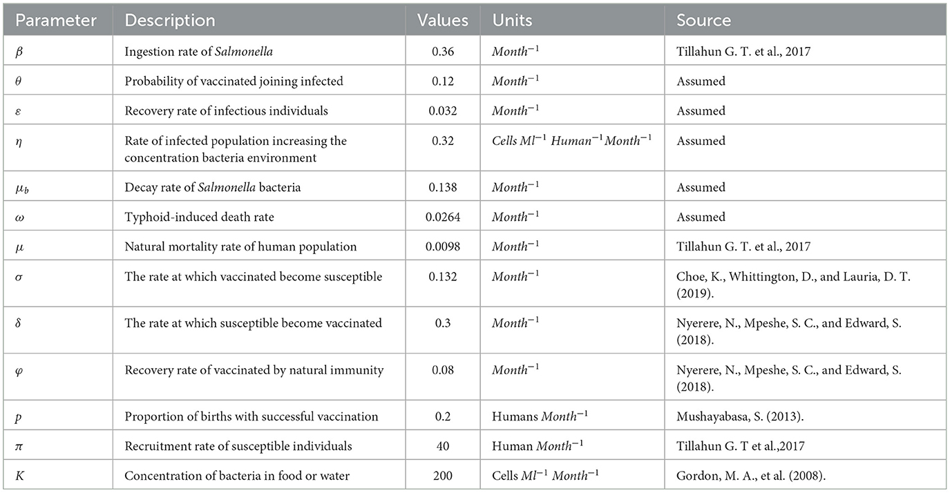
Table 1. Description of parameters in the Model (1) and their values.

The model comprises the following system of differential equations based on the presumptions and the compartmental diagram in Figure 1 with initial conditions S(0)>0, V(0)≥0, I(0)≥0, R(0)≥0, B(0)≥0.

$\begin{array}{ll}\begin{array}{c}\frac{dS}{dt}=\left(1-p\right)\pi +\sigma V-\lambda S-(\delta +\mu )S\\ \frac{dV}{dt}=p\pi +\delta S-\theta \lambda V-\left(\sigma +\phi +\mu \right)V\\ \frac{dI}{dt}=\lambda S+\theta \lambda V-\left(\epsilon +\omega +\mu \right)I\\ \frac{dR}{dt}=\phi V+\epsilon I-\mu R\\ \frac{dB}{dt}=\eta I-{\mu }_{b}B\end{array}\}& (1)\end{array}$

Figure 1

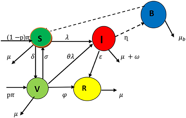
Figure 1. Schematic representation of typhoid fever transmission dynamics through compartments.

3 Model analysis

3.1 Invariant region and positivity of the solutions

Theorem 3.1: The model's possible solutions are all uniformly bounded within the proper subset Ω = Ω_H×Ω_B where Ω_H $=\left\{(S,V,I,R)\in {R^4}_{+}:N(t)\le \frac{\pi }{u}\right\}$ is a subset for human population and ${\Omega }_B=\left\{B\in R_{+}:B\le n\frac{\pi }{u}\right\}$ is a subset associated with environmental bacterial infections.

Proof: N = S+V+I+R yields the entire human population N (t) under the initial conditions N(0) = N₀ = S₀+V₀+I₀+R₀ and B (0) = B₀ for S.typhi bacteria in the environment. Establishing a differentiation of N and with respect to time (t), we obtain

$\begin{array}{ll}\frac{dN}{dt}=\frac{dS}{dt}+\frac{dV}{dt}+\frac{dI}{dt}+\frac{dR}{dt}& (2)\end{array}$

Substituting Equation 1 in place of Equation 2 and assuming no disease-induced death rate (i.e making = ω = 0 ), we have

$\begin{array}{ll}\frac{dN}{dt}\le \pi -uN(t)& (3)\end{array}$

Rearranging and integrating both sides of Equation 3, we get

$\begin{array}{ll}N(t)\le \frac{\pi }{u}+\left(N_O-\frac{\pi }{u}\right)e^{-ut}& (4)\end{array}$

When time moves to ∞ in Equation 4, N(t) converges to π/u; this indicates that there are feasible model solutions for the local population.

$\begin{array}{ll}{\text{Ω}}_{H=}\left\{(S,V,I,R)\in {R^4}_{+}:N(t)\le \frac{\pi }{u}\right\}& (5)\end{array}$

For bacteria environment since N(t) ≤ π/u, it means that I ≤ π/u. We have from the last Equation 1 that

$\begin{array}{ll}\frac{dB}{dt}=\eta I-{\mu }_{b}B\le \eta N-{\mu }_{b}B\le \eta \frac{\pi }{\mu }-{\mu }_{b}B& (6)\end{array}$

Evaluating Equation 6 with B(0) = B₀ as a stating condition yields

$\begin{array}{ll}B(t)\le \frac{\eta \pi }{\mu {\mu }_b}+\left(B_0-\frac{\eta \pi }{\mu {\mu }_b}\right)e^{-{\mu }_{b}t}& (7)\end{array}$

As t tends to infinity, Equation 7 becomes $B(t)\le \frac{n\pi }{\mu }$. Therefore, the feasible solution of the bacteria population enters the region

$\begin{array}{ll}{\text{Ω}}_B=\left\{B\in R_{+}:B\le \frac{n\pi }{\mu }\right\}& (8)\end{array}$

Therefore, from Equations 5, 8 the feasible region of the model is given by

$\begin{array}{l}\Omega ={\Omega }_H\times {\Omega }_B=\{\left(S,V,I,R\right)\in R_{+}^4:N\left(t\right)\le \frac{\pi }{\mu },B\in R_{+}\\ :B\le \frac{\pi n}{\mu }\}\end{array}$

Theorem 3.2: Let $\Omega =\{\left(S,V,I,R,B\right)\in R_{+}^{5}S\left(0\right)>0,V\left(0\right)\ge 0,I\left(0\right)\ge 0,R\left(0\right)\ge 0,B\left(0\right)\ge O\}$ then the solution { S, V, I, R, B} are positive for all t≥ 0.

Proof: From the fifth equation of model (1)

$\begin{array}{ll}\frac{dB}{dt}\ge -B{\mu }_b& (9)\end{array}$

By using comparison theorem, Equation 9 is solved as, we get (t) $\ge e^{-{\mu }_{b}t+C}$,

$\begin{array}{l}B(t)\ge B(0).e^{-{\mu }_{b}t}\ge 0,whereB(0)=e^{C}att=0\end{array}$

From the first equation of model (1), we have

$\begin{array}{ll}\frac{dS}{dt}\ge -(\frac{\beta B}{K+B}+(\delta +\mu ))S& (10)\end{array}$

By comparison theorem, integrating Equation 10 with initial conditions S(0) = S₀ yields

$\begin{array}{l}S(t)\ge S_0{e}^{-\left(\frac{\beta B}{K+B}+(\delta +\mu )\right)t}\ge 0\end{array}$

After substituting the solution of B(t), we get

$\begin{array}{l}S(t)\ge S_0{e}^{-\left(\frac{\beta B(0).e^{-{\mu }_{b}t}}{K+B(0).e^{-{\mu }_{b}t}}+(\delta +\mu )\right)t}\ge 0\end{array}$

Similarly, we can prove the positivity of the other variables as

$\begin{array}{l}V\left(t\right)\ge V_0{e}^{-\left(\frac{\text{β}B\left(0\right).e^{-{\mu }_{b}t}}{K+B\left(0\right).e^{-{\mu }_{b}t}}+\left(\sigma +\phi +\mu \right)\right)t}\ge 0,I(t)\\ \ge I(0)e^{-\left(\epsilon +\eta +\omega +\mu \right)}\ge 0\end{array}$

and (t) ≥R(0) e^−μt≥0. Thus S(t), V(t), I(t), R(t,) and B(t) are positive for all t ≥0

3.2 Typhoid fever-free equilibrium

We denote the typhoid fever-free equilibrium by E⁰. By setting the right-hand side of the equations in system (1) to zero and simultaneously solving for the uninfected compartments S, V, and R, we obtain the typhoid fever-free equilibrium as:

$\begin{array}{ll}{E}^0=(S^0,V^0,I^0,{R,}^0{B}^0)=(\frac{\pi k_3}{k_4},\frac{\pi k_5}{k_6},0,\frac{\varphi \pi k_5}{\mu k_6},0)& (11)\end{array}$

where k₁ = δ+μ k₂ = σ+φ+μ, k₃ = − k₂(1−p)−p σ, k₄= σ δ−k₂k₁;

$\begin{array}{l}{k}_5=-k_4(1-p)-k_1{k}_{3}and{k}_6=\sigma k_4\end{array}$

3.3 Effective reproduction number

When an infected person enters a vaccinated community, the average number of secondary cases produced is known as the effective reproduction number R_Eff. It is computed using the next-generation matrix approach, J [18, 19]. Using the principle

$\begin{array}{ll}F=\left\{\begin{array}{c}\frac{\beta BS}{K+B}+\frac{\theta \beta BV}{K+B}\\ 0\end{array}\right\}andV=\left\{\begin{array}{l}(\epsilon +\omega +\mu )I\\ -\eta I+{\mu }_{b}B\end{array}\right\}& (12)\end{array}$

Then, from Equation 12, the Jacobian matrices evaluated at the FFEP are obtained as:

$f=\left[\begin{array}{cc}0& \frac{\beta (S^0+\theta V^0)}{K}\\ 0& 0\end{array}\right],v=\left[\begin{array}{cc}\epsilon +\omega +\mu & 0\\ -\eta & {\mu }_b\end{array}\right]$

Computing the inverse of v, we get

$\begin{array}{l}{v}^{-1}=\frac{1}{\det \left(v\right)}Adjoint\left(v\right)=\frac{1}{{\mu }_b\left(\epsilon +\omega +\mu \right)}\left[\begin{array}{cc}{\mu }_b& 0\\ \eta & \epsilon +\omega +\mu \end{array}\right]\\ =\left[\begin{array}{cc}\frac{1}{(\epsilon +\omega +\mu )}& 0\\ \frac{\eta }{{\mu }_b\left(\epsilon +\omega +\mu \right)}& \frac{1}{{\mu }_b}\end{array}\right]\end{array}$

Then using the principle, the next-generation matrix is given by

$\begin{array}{l}G=f{v}^{-1}=\left[\begin{array}{cc}0& \frac{\beta (S^0+\theta V^0)}{K}\\ 0& 0\end{array}\right]\left[\begin{array}{cc}\frac{1}{(\epsilon +\omega +\mu )}& 0\\ \frac{\eta }{{\mu }_b\left(\epsilon +\omega +\mu \right)}& \frac{1}{{\mu }_b}\end{array}\right]\\ =\left[\begin{array}{cc}\frac{\beta \eta (S^0+\theta V^0)}{K{\mu }_b\left(\epsilon +\omega +\mu \right)}& \frac{\beta (S^0+\theta V^0)}{K{\mu }_b}\\ 0& 0\end{array}\right]\end{array}$

The eigenvalue of a matrix G determined by det (G- λI) = 0 and the dominant eigenvalue becomes the effective reproduction number of the model. Hence,

$\begin{array}{l}{R}_{Eff}=\frac{\text{βηπ}(\delta \theta +\sigma +\phi +u)(1-p)+p(\theta (\delta +u)+\sigma )}{k{\text{μ}}_b(\epsilon +\omega +\mu )\left[\mu (\mu +\delta +\phi +u)+\delta \phi \right]}\end{array}$

3.4 Local stability typhoid fever-free equilibrium point

Theorem 3.3: The typhoid fever-free equilibrium E⁰ of the model (1) is locally asymptotically stable (LAS) if R_Eff <1, otherwise it is unstable.

Proof: The Jacobian matrix of the model in Equation 1 is given by

$\begin{array}{l}J=\left[\begin{array}{ccccc}\frac{\beta B}{K+B}-(\delta +\mu )& \sigma & 0& 0& \frac{-\beta S}{K+B}+\frac{\beta B}{{(K+B)}^2}\\ \delta & \frac{\theta \beta B}{K+B}-(\sigma +\phi +\mu )& 0& 0& -\frac{\theta \beta V}{K+B}+\frac{\theta \beta BV}{{(K+B)}^2}\\ \frac{\beta B}{K+B}& \frac{\theta \beta B}{K+B}& -(\epsilon +\omega +\mu )& 0& \frac{\beta S}{K+B}-\frac{\beta BS}{{(K+B)}^2}+\frac{\theta \beta BV}{K+B}-\frac{\theta \beta BV}{{(K+B)}^2}\\ 0& \phi & \epsilon & -u& 0\\ 0& 0& \eta & 0& -{\mu }_b\end{array}\right]\end{array}$

If we evaluated at the typhoid fever-free equilibrium point E⁰, we get

$\begin{array}{ll}J=\left[\begin{array}{ccccc}-(\delta +\mu )& \sigma & 0& 0& \frac{-\beta S^0}{K}\\ \delta & -(\sigma +\phi +\mu )& 0& 0& -\frac{\theta \beta V^0}{K}\\ 0& 0& -(\epsilon +\omega +\mu )& 0& \frac{\beta S^0}{K}+\frac{\theta \beta V^0}{K}\\ 0& \phi & \epsilon & -\mu & 0\\ 0& o& \eta & 0& -{\mu }_b\\ \end{array}\right]& (13)\end{array}$

To make the proof more clarified, the Jacobian is block-triangular; this allows us to partition it and compute eigenvalues separately. Let us use submatrix, as infected and healthy:

Healthy states (S,V,R):

$\begin{array}{l}{J}_1=\left[\begin{array}{ccc}-(\delta +\mu )& \sigma & 0\\ \delta & -(\sigma +\phi +\mu )& 0\\ 0& 0& -\mu \\ \end{array}\right]\end{array}$

Infected states (I,B):

$\begin{array}{l}{J}_2=\left[\begin{array}{cc}-(\epsilon +\omega +\mu )& \frac{\beta S^0}{K}+\frac{\theta \beta V^0}{K}\\ \eta & -{\mu }_b\\ \end{array}\right]\end{array}$

Since J₁ is a lower triangular, the eigenvalues are its diagonal entries:

$\left(-u-\lambda \right)\left|\begin{array}{cc}-\left(\delta +\mu \right)-\lambda & \sigma \\ \delta & \left(\sigma +\phi +\mu \right)-\lambda \end{array}\right|=0$

The first eigenvalue is −u = λ₁ and the other eigenvalues are obtained from the characteristic equation given by

$\begin{array}{l}(-(\delta +\mu )-\lambda )(-(\sigma +\varphi +\mu )-\lambda )-\sigma \delta =0.\\ {\lambda }^2+A\lambda +B=0\end{array}$

where

$\begin{array}{l}A=\delta +\mu +\sigma +\varphi +\mu >0,\\ B=\delta \sigma +\delta \varphi +\delta \mu +\mu \sigma \\ +\mu \varphi +{\mu }^2-\sigma \delta =\delta \varphi +\delta \mu +\mu \sigma +\mu \varphi +{\mu }^2>0\end{array}$

Hence the eigenvalues of the matrix J₁are negative from the Hurwitz criterion.

The eigenvalues of J₂ determine the stability of the infected states. The characteristic equation is:

$\left|\begin{array}{cc}-\left(\epsilon +\omega +\mu \right)-\lambda & \frac{\beta S^0}{K}+\frac{\text{θβ}{V}^0}{K}\\ \eta & -{\mu }_b-\lambda \end{array}\right|=0$

The corresponding characteristic equation is given by

$\begin{array}{l}{\lambda }^2+\left(\epsilon +\mu +\omega +{\mu }_b\right)\lambda +\left(\epsilon +\mu +\omega \right){\mu }_b-\frac{\beta \eta (S^0+\theta V^0)}{K}\\ =0& (14)\end{array}$

where

$\begin{array}{l}{a}_1=\epsilon +\mu +\omega +{\mu }_b>0,\\ a_2=\left(\epsilon +\mu +\omega \right){\mu }_b-\frac{\beta \eta (S^0+\theta V^0)}{K},\\ =\left(\epsilon +\mu +\omega \right){\mu }_b\left(1-\frac{\beta \eta (S^0+\theta V^0)}{K{\mu }_b\left(\epsilon +\mu +\omega \right)}\right)\\ =\left(\epsilon +\mu +\omega \right){\mu }_b\left(1-R_{Eff}\right)>0\end{array}$

Therefore, the disease-free equilibrium point is LAS whenever R_Eff <1.

3.5 Global stability of typhoid fever-free equilibrium

We utilized the Castillo-Chávez et al. [20] technique to show the globally stability of typhoid fever-free equilibrium as it used by Alemneh and Alemu [21]. The Castillo-Chávez et al. [20] method divides the population into two as

$\begin{array}{l}\frac{dx}{dt}=F_1\left(x,z\right),\\ \frac{dz}{dt}=F_2(x,z),F_2(x,0)=0& (15)\end{array}$

xϵℝ³ shows the number of uninfected individuals (susceptible, vaccinated, and recovered) while zϵℝ² is the number of infected human individuals and bacteria in the environment. Let the typhoid fever-free equilibrium be denoted by (x⁰, 0). The two basic axioms that guarantee the global stability of typhoid fever-free equilibrium are:

H₁: For $\frac{dx}{dt}=F_1(x,0)$, x⁰, is globally asymptotically stable.

$H_2:F_2(x,z)=Az-\overline{F_2}(x,z)$ where $\overline{F_2}(x,z)\ge 0$ for (x, z) ϵ Ω and the

matrix A = D_z $F_2(x^0,0)$ denotes an M-matrix.

Theorem 3.4: The typhoid fever-free equilibrium point of the model (1) is globally asymptotically stable (GAS) if the system in Equation 15 satisfies the axioms (H₁) and (H₂) for R_Eff <1 otherwise unstable.

Proof: Let x = (S(t),V(t), R(t)) and z = (I(t), B(t)) represent the number of uninfected and infected individuals, respectively. Define E⁰ = (x⁰, 0), x⁰= $(\frac{\pi k_3}{k_4},\frac{\pi k_5}{k_6},\frac{\varphi }{\text{π}}{k}_5\mu k_6)$ .

$\begin{array}{ll}{F}_1(x,z)=\left(\begin{array}{c}(1-p)\pi +\sigma V-\frac{\beta B}{K+B}S-(\delta +\mu )S\\ p\pi +\delta S-\frac{\theta \beta B}{K+B}V-(\sigma +\phi +\mu )V\\ \phi V+\epsilon I-\mu R\end{array}\right)& (16)\end{array}$

The reduced system according to the condition H_1: becomes

$\begin{array}{l}\frac{dS}{dt}=\left(1-p\right)\pi +\sigma V-\left(\delta +\mu \right)S\\ \frac{dV}{dt}=p\pi +\delta S-\left(\sigma +\phi +\mu \right)V\\ \frac{dR}{dt}=\phi V-\mu R& (17)\end{array}$

Solving Equation 17 one by one, we have

$\begin{array}{ll}S(t)=\frac{\left[(1-p)\pi +\sigma V^0\right]}{(\delta +\mu )}+\frac{c}{e^{(\delta +\mu )t}}& (18)\end{array}$

From Equation 18, as t approaches ∞, $\frac{c}{e^{(\delta +\mu )t}}$ approaches to zero.

Substitute $V^0=\frac{\pi (\sigma +\mu P)}{\sigma (\phi +\mu )+\mu (\sigma +\phi +\mu )}$ we get $S(t)=(\frac{(1-p)\pi +\sigma (\frac{\pi (\sigma +\mu P)}{\delta (\phi +\mu )+\mu (\sigma +\phi +\mu )})}{(\delta +\mu )})$

$\begin{array}{l}\left(\frac{\left(1-p\right)\pi +\sigma \left(\frac{\pi \left(\sigma +\mu P\right)}{\delta \left(\phi +\mu \right)+\mu \left(\sigma +\phi +\mu \right)}\right)}{\left(\delta +\mu \right)}\right)\mathrm{=}\\ \frac{\pi \left(\sigma +(\phi +\mu )(1-p)\right)}{\delta \left(\phi +\mu \right)+\mu \left(\sigma +\phi +\mu \right)}=S^0\end{array}$

Similarly, we show for R and V

$\begin{array}{l}\underset{t\to \infty }{\lim }[p\pi +\delta \left(\frac{\pi (\sigma +\left(\phi +\mu \right)\left(1-p\right))}{\delta \left(\phi +\mu \right)+\mu (\sigma +\phi +\mu )}\right)+\frac{C}{e^{\left(\sigma +\phi +\mu \right)t}}\\ =V^{0}and\underset{t\to \infty }{\lim }\frac{\phi \pi (\sigma +\mu P)}{\mu \left(\delta \left(\phi +\mu \right)+\mu (\sigma +\phi +\mu \right)}+\frac{c}{e^{\text{μ}t}}=R^0\end{array}$

Therefore, as → ∞ x(t) → x⁰. Thus, x⁰ = $(\frac{\pi k_3}{k_4},\frac{\pi k_5}{k_6},\frac{\varphi \text{π}{k}_5}{\mu k_6})$ is globally asymptotically stable. Now to prove the second condition, we have

$\begin{array}{ll}{F}_2(x,z)=\left(\begin{array}{c}\frac{\text{β}B}{K+B}S+\frac{\text{θβ}B}{K+B}V-(\epsilon +\omega +\mu )I\\ \eta I-{\mu }_{b}B\\ \end{array}\right)& (19)\end{array}$

Using condition H₂ the matrix A = D_z F₂(x, 0) of Equation 19, evaluated at typhoid fever-free equilibrium point given by

$\begin{array}{l}A=\left[\begin{array}{cc}-(\epsilon +\omega +\mu )& \frac{\beta K{S}^0}{K}+\frac{\theta \beta V^0}{K}\\ \eta & -{\mu }_b\end{array}\right]\end{array}$

Hence from $\overline{F_2}(x,z)=AZ-F_2(x,z)$, we have

$\begin{array}{l}\overline{F_2}(x,z)=\left[\begin{array}{c}\beta B(\frac{S^0}{K}-\frac{S}{K+B})+\beta B(\frac{V^0}{K}-\frac{V}{K+B})\\ 0\end{array}\right]\end{array}$

Since S⁰ ≥ S, V⁰≥ V and $\frac{1}{K}\ge \frac{1}{K+B}$, thus $\overline{F_2}(x,z)\ge$ 0 (x, z)ϵΩ. Thus, H_1: and H_2: are satisfied, so, the typhoid fever-free equilibrium point E⁰ is GAS. This result is also supported by the theorem 3.6 in Section 3.6.

3.6 Endemic equilibrium point

The endemic equilibrium point exists when R_Eff > 1. Let E¹ = (S^*, V^*, I^*, R^*, B^*) ≠0 denote the endemic equilibrium of model (1) and it is obtained by setting all the derivatives in model (1) to zero, i.e.,

$\begin{array}{l}\frac{dS}{dt}=\frac{dV}{dt}=\frac{dI}{dt}=\frac{dR}{dt}=\frac{dB}{dt}=0\end{array}$

We obtained

$\begin{array}{l}{V}^{\ast }=\frac{\left(\epsilon +\omega +\mu \right)\left(k{\mu }_b+\eta I^{\ast }\right)-\beta \eta \pi }{\text{βη}\left(\sigma -\left(\phi +\mu \right)+\mu \theta \right)},\\ S^{\ast }=\frac{\left(\epsilon +\omega +\mu \right)\left(k{\mu }_b+\eta I^{\ast }\right)\left[\sigma -\left(\phi +\mu \right)\right]-\beta \eta \pi }{\text{βη}\left(\sigma -\left(\phi +\mu \right)+\mu \theta \right)},\end{array}$

$R^{\ast }=\frac{\phi \left(\epsilon +\omega +\mu \right)\left(k{\text{μμ}}_b+\text{ημ}{I}^{\ast }\right)-\phi \beta \eta \pi +\beta \eta \left(\sigma -\left(\phi +\mu \right)+\mu \theta \right)I^{\ast }}{\text{ηβμ}\left(\sigma -\left(\phi +\mu \right)+\mu \theta \right)},B^{\ast }=\frac{\eta }{{\mu }_b}{I}^{\ast }$

Where I^* is the positive root of the following quadratic function

$\begin{array}{ll}{\eta }^{2}MT{I^{*}}^2+Q{I}^{*}+L=0& (20)\end{array}$

with

$\begin{array}{l}M=\left(\epsilon +\omega +\mu \right),T=-\sigma \delta +\delta \phi +\delta \mu +\mu \phi +{\mu }^2\\ Q=\eta [\left(1-p\right)\pi r+\sigma \eta \beta \pi -rp-\delta k{\mu }_b\sigma M\delta k{\mu }_{b}M\\ ++\delta k{\mu }_b\mu M-2\mu k{\mu }_b\sigma M+2k{\mu }_b\phi M+2{\mu }^{2}k{\mu }_{b}M\\ -\delta Mk{\mu }_b\sigma +\delta \phi Mk{\mu }_b+\delta \phi Mk{\mu }_b+\delta \theta \beta \eta \pi -\mu Mk{\mu }_b\sigma \\ +\mu \phi Mk{\mu }_b+{\mu }^{2}M{\mu }_b+\mu M\eta ]\\ L=\left(1-p\right)\pi rk{\mu }_b+\delta k^2{\mu }_b^{2}M\mu \\ -\delta k{\mu }_b\text{βπ}\eta +\sigma \eta Mk{\mu }_b-\delta k^2{\mu }_b^{2}M\sigma \\ +\delta k^2{\mu }_b^{2}M\phi +\delta k^2{\mu }_b^{2}M\mu -\delta k{\mu }_b\text{θβ}\eta \pi -2\mu k^2{\mu }_b^{2}M\sigma \\ +2\mu k^2{\mu }_b^{2}M\phi +2{\mu }^2{k}^2{\mu }_b^{2}M+2{\mu }_b\text{βπηθ}\end{array}$

Theorem 3.5: For R_Eff>1, there is a unique endemic equilibrium point and no endemic equilibrium elsewhere.

Proof: For the disease to be endemic $\frac{dI}{dt}>0,\frac{dB}{dt}>0$. Hence,

$\begin{array}{l}\frac{\text{β}BS}{K+B}+\frac{\text{θβ}B}{K+B}V>\left(\epsilon +\omega +\mu \right)I\Rightarrow \left(\epsilon +\omega +\mu \right)I\\ \\ <\frac{\text{β}BS}{K+B}+\frac{\text{θβ}B}{K+B}V\\ \Rightarrow I<\frac{\beta BS+\theta \beta BV}{(K+B)\left(\epsilon +\omega +\mu \right)}and\text{ η}I>{\mu }_{b}B\Rightarrow {\mu }_{b}B& (21)\end{array}$

$\begin{array}{l}<\text{η}I\Rightarrow B<\frac{\text{η}I}{{\mu }_b},\\ \Rightarrow 1<\frac{\text{ηβ}{S}^0}{{\mu }_b(K+B^0)\left(\epsilon +\omega +\mu \right)}\\ +\frac{\text{ηθβ}{V}^0}{{\mu }_b(K+B^0)\left(\epsilon +\omega +\mu \right)}& (22)\end{array}$

Since B⁰≥0, then Equation 22 is reduced to

$\begin{array}{l}1<\frac{\text{ηβ}{S}^0+\text{ηθβ}{V}^0}{{\mu }_{b}k(\epsilon +\omega +\mu )}\Rightarrow 1<R_{Eff}implies{R}_{Eff}>1\end{array}$

3.7 Local stability of EEP and bifurcation analysis

The local stability of the endemic equilibrium is established by demonstrating the existence of a forward bifurcation of the system using the center manifold technique, which is employed due to the mathematical difficulty of endemic equilibrium stability. A forward bifurcation indicates that the endemic equilibrium is locally asymptotically stable if R_Eff> 1 but near unity.

Using the approach of the center manifold theory [20, 22], we demonstrated the bifurcation analysis of the typhoid fever model in Equation 1. Let β = β^* be a bifurcation parameter at R_Eff = 1, so that

$\beta ={\beta }^{\ast }=\frac{k{\text{μ}}_b\left(\epsilon +\omega +\mu \right)[\mu \left(\delta +\phi +\sigma +\mu \right)+\delta \phi ]}{\text{ηπ}\left(\delta \theta +\mu +\sigma +\phi )\left(1-p\right)+p(\theta \left(\delta +\mu \right)+\sigma )\right)},$

and we assume that S = z₁, V= z₂, I = z₃, R = z₄, B = z₅ and the model (1) is given by

$\begin{array}{ll}\{\begin{array}{c}(1-p)\pi +\sigma z_2-\frac{\beta z_5{z}_1}{K+z_5}-\left(\delta +\mu \right)z_1=0\\ p\pi +\delta z_1-\frac{\text{θβ}{z}_5{z}_2}{K+z_5}-\left(\sigma +\phi +\mu \right)z_2=0\\ \frac{\beta z_5{z}_1}{K+z_5}+\frac{\text{θβ}{z}_5{z}_2}{K+z_5}-\left(\epsilon +\omega +\mu \right)z_3=0\\ \phi z_2+\epsilon z_3-\mu z_4=0\\ \eta z_3-{\mu }_b{z}_5=0\end{array}& (23)\end{array}$

The Jacobian matrix of the system [9] around the typhoid-free equilibrium point evaluated at R_Eff = 1 is

$J=\left[\begin{array}{ccccc}-\left(\delta +\mu \right)& \sigma & 0& 0& \frac{-\beta z_1^0}{k}\\ \delta & -\left(\sigma +\phi +\mu \right)& 0& 0& -\frac{\theta \beta z_2^0}{k}\\ 0& 0& -(\epsilon +\omega +\mu )& 0& \frac{\beta z_1^0}{k}+\frac{\theta \beta z_2^0}{k}\\ 0& \phi & \epsilon & -\mu & 0\\ 0& o& \eta & 0& -{\mu }_b\end{array}\right]$

The right eigenvector W$={(w_{1,}{w}_{2,}{w}_{3,}{w}_{4,}{w}_{5,})}^t$ associated with this simple zero eigenvalue can be obtained from JW = 0.

$\begin{array}{l}{w}_2=\left[\frac{\text{δβ}{z}_1^0+\theta \beta z_2^0\left(\delta +\mu \right)}{k\left(\delta \sigma -\left(\delta +\mu \right)\left(\sigma +\phi +\mu \right)\right)}\right]w_5,\\ w_1=\left[\frac{\text{σθβ}{z}_2^0+\beta z_1^0\left(\sigma +\phi +\mu \right)}{k\left(\delta \sigma -\left(\delta +\mu \right)\left(\sigma +\phi +\mu \right)\right)}\right]w_5,\\ w_3=\frac{{\mu }_b}{\eta }{w}_5,w_4=\frac{1}{\text{ μη}}\left[\frac{\varphi x}{y}+\frac{\epsilon {\mu }_b}{\eta }\right]w_5\end{array}$

where $x=\delta \beta {z_1}^0+\theta \beta {z_2}^0(\delta +\mu )$ and y = k(δσ−(δ+μ)((σ+φ+μ). The left eigenvector = ${(v_{1,}{v}_{2,}{v}_{3,}{v}_{4,}{v}_{5,})}^t$, associated with this simple zero eigenvalue, can be obtained from VJ = 0 and given by

$\begin{array}{l}{v}_1=0,v_2=0v_4=0v_3=v_3>0and{v}_5=\frac{(\epsilon +\eta +\omega +\mu )}{\eta }{v}_3\\ \end{array}$

We do not require the derivative of f₁, f₂, and f₄since the first, second, and fourth components of V are all zero. Additionally, since the expression for f₅ is linear, all its second-order partial derivatives are zero. From the derivatives the only ones that are non-zero are derivatives from f₃ and are listed below.

$\begin{array}{l}\frac{{\partial }^2{f}_3(E^0)}{\partial z_2\partial z_5}=\frac{{\partial }^2{f}_3(E^0)}{\partial z_5\partial z_2}=\frac{\theta \beta }{k}\frac{{\partial }^2{f}_3(E^0)}{\partial z_1\partial z_5}=\frac{{\partial }^2{f}_3(E^0)}{\partial z_5\partial z_1}\\ =\frac{\beta }{k}and\frac{{\partial }^2{f}_3(E^0)}{\partial z_5\partial z_{\beta }}=(\frac{{z_1}^0}{k}+\frac{\theta {z_2}^0}{k})\end{array}$

The signs of the derived bifurcation coefficients a and b reflect the direction of the bifurcation at R_Eff = 1.

$\begin{array}{l}a={\displaystyle \sum _{k,i,j=1}^5{v}_k{w}_i{w}_j}\frac{{\partial }^2{f}_k}{\partial x_i\partial x_j}=-\frac{2v_3{w}_5^2\beta }{k^2}\\ \left[\frac{\text{δθβ}{z}_1^0+{\theta }^2\beta z_2^0\left(\delta +\mu \right)+\sigma \theta \beta z_2^0+\beta z_1^0\left(\sigma +\phi +\mu \right)}{\left(\left(\phi +\mu \right)\left(\delta +\mu \right)+\mu \sigma \right)}\right]<0\\ b={\displaystyle \sum _{k,i=1}^5{v}_k{w}_i}\frac{{\partial }^2{f}_k}{\partial x_i\partial x_{\beta }}=v_3{w}_5\frac{{\partial }^2{f}_3(E_{0)}}{\partial z_5\partial \beta }\\ =v_3{w}_5\left(\frac{z_1^0}{k}+\frac{\theta z_2^0}{k}\right)>0,\end{array}$

Consequently, a supercritical bifurcation takes place in the model since the bifurcation coefficient, b, is inherently positive and a is negative. Thus, the theorem is inferred from the outcome.

Theorem 3.6. Whenever R_Eff > 1 but near unity, the following are true:

i. The endemic equilibrium is locally asymptotically stable.

ii. The model illustrates forward bifurcation.

iii. The DFE point is globally asymptotically stable.

3.8 Endemic equilibrium point global stability

Theorem 3.7: The point E^* is globally asymptotically stable if R_Eff>1, otherwise unstable.

Proof: We construct the Lyapunov function given by

$\begin{array}{l}L=(S-S^{\ast }-S^{\ast }\ln \frac{S}{S^{\ast }})+(V-V^{\ast }-V^{\ast }\ln \frac{V}{V^{\ast }})\\ +(I-I^{\ast }-I^{\ast }\ln \frac{I}{I^{\ast }})+\frac{\beta B^{\ast }{S}^{\ast }}{\eta I^{\ast }(K+B^{\ast )}}(B-B^{\ast }-B^{\ast }\ln \frac{B}{B^{\ast }})& (24)\end{array}$

Taking the derivative of L in Equation 24 alongside the solutions of equation of model (1) yields

$\begin{array}{l}\frac{dL}{dt}=\left(1-\frac{S^{\ast }}{S}\right)\frac{dS}{dt}+\left(1-\frac{V^{\ast }}{V}\right)\frac{dV}{dt}+\left(1-\frac{I^{\ast }}{I}\right)\frac{dI}{dt}\\ +\frac{\beta B^{\ast }{S}^{\ast }}{\eta I^{\ast }(K+B^{\ast )}}\left(1-\frac{B^{\ast }}{B}\right)\frac{dB}{dt}& (25)\end{array}$

At endemic equilibrium steady state, we have

$\begin{array}{ll}\begin{array}{c}\left(1-p\right)\pi =-\sigma V^{\ast }+\frac{\beta B^{\ast }}{K+B^{\ast }}{S}^{\ast }+\left(\delta +\mu \right)S^{\ast }\\ p\pi =-\delta S^{\ast }+\frac{\text{θβ}{B}^{\ast }}{K+B^{\ast }}{V}^{\ast }+\left(\sigma +\phi +\mu \right)V^{\ast }\\ \frac{\frac{\beta B^{\ast }}{K+B^{\ast }}{S}^{\ast }+\frac{\text{θβ}{B}^{\ast }}{K+B^{\ast }}{V}^{\ast }}{I^{\ast }}=\left(\epsilon +\omega +\mu \right)\\ {\mu }_b=\frac{\eta I^{\ast }}{B^{\ast }}\end{array}\}& (26)\end{array}$

Substituting Equation 25 in Equation 26 and simplify

$\begin{array}{l}\left(1-\frac{S^{\ast }}{S}\right)\frac{dS}{dt}=\left(1-\frac{S^{\ast }}{S}\right)\left[-\sigma V^{\ast }+\frac{\beta B^{\ast }}{K+B^{\ast }}{S}^{\ast }+\left(\delta +\mu \right)S^{\ast }+\sigma V-\frac{\text{β}B}{K+B}S-\left(\delta +\mu \right)S\right]\\ \le \frac{\beta B^{\ast }{S}^{\ast }}{K+B^{\ast }}\left(1-\frac{S^{\ast }}{S}\right)\left[(1-\frac{BS\left(K+B^{\ast }\right)}{S^{\ast }{B}^{\ast }\left(K+B\right)})\right]\\ \left(1-\frac{V^{\ast }}{V}\right)\frac{dV}{dt}=\left(1-\frac{V^{\ast }}{V}\right)\left[-\delta S^{\ast }+\frac{\text{θβ}{B}^{\ast }}{K+B^{\ast }}{V}^{\ast }+\left(\sigma +\phi +\mu \right)V^{\ast }+\delta S-\frac{\text{θβ}B}{K+B}V-\left(\sigma +\phi +\mu \right)V\right]\\ \le \frac{\text{θβ}{B}^{\ast }{V}^{\ast }}{K+B^{\ast }}\left(1-\frac{V^{\ast }}{V}\right)\left[(1-\frac{BV(K+B^{\ast })}{B^{\ast }{V}^{\ast }(K+B)})\right]\\ \left(1-\frac{I^{\ast }}{I}\right)\frac{dI}{dt}=\left(1-\frac{I^{\ast }}{I}\right)\left[\frac{\text{β}B}{K+B}S+\frac{\text{θβ}B}{K+B}V-\left(\frac{\beta B^{\ast }}{K+B^{\ast }}{S}^{\ast }+\frac{\text{θβ}{B}^{\ast }}{K+B^{\ast }}{V}^{\ast }\right)\frac{I}{I^{\ast }}\right]\\ =\left(1-\frac{I^{\ast }}{I}\right)\left[\frac{\beta B^{\ast }{S}^{\ast }}{K+B^{\ast }}\left(\frac{BS\left(K+B^{\ast }\right)}{B^{\ast }{S}^{\ast }\left(K+B\right)}-\frac{I}{I^{\ast }}\right)+\frac{\text{θβ}{B}^{\ast }{V}^{\ast }}{K+B^{\ast }}\left(\frac{BV\left(K+B^{\ast }\right)}{B^{\ast }{V}^{\ast }\left(K+B\right)}-\frac{I}{I^{\ast }}\right)\right]\\ \frac{\beta B^{\ast }{S}^{\ast }}{\eta I^{\ast }(K+B^{\ast )}}\left(1-\frac{B^{\ast }}{B}\right)\frac{dB}{dt}=\frac{\beta B^{\ast }{S}^{\ast }}{\eta I^{\ast }(K+B^{\ast )}}\left(1-\frac{B}{B^{\ast }}\right)\left[\text{η}I-\frac{\eta I^{\ast }}{B^{\ast }}B\right]=\frac{\beta B^{\ast }{S}^{\ast }}{(K+B^{\ast )}}(1+\frac{I}{I^{\ast }}-\frac{B}{B^{\ast }}-\frac{B^{\ast }I}{B{I}^{\ast }})\end{array}$

For the function $ℒ(x)=1-x+lnx$, we know that x > 0 leads to $ℒ(x)\le 0.$ And if x = 1, then $ℒ(x)=0.$ Note that

$\begin{array}{l}\frac{\beta B^{\ast }{S}^{\ast }}{K+B^{\ast }}\left(1-\frac{S^{\ast }}{S}\right)\left[\left(1-\frac{BS\left(K+B^{\ast }\right)}{S^{\ast }{B}^{\ast }\left(K+B\right)}\right)\right]+\frac{\beta B^{\ast }{S}^{\ast }}{K+B^{\ast }}\left(1-\frac{I^{\ast }}{I}\right)\left[\left(\frac{BS\left(K+B^{\ast }\right)}{B^{\ast }{S}^{\ast }\left(K+B\right)}-\frac{I}{I^{\ast }}\right)\right]==\frac{\beta B^{\ast }{S}^{\ast }}{K+B^{\ast }}\left[2-\frac{S^{\ast }}{S}-\frac{I}{I^{\ast }}+\frac{B\left(K+B^{\ast }\right)}{B^{\ast }\left(K+B\right)}-\frac{BS\left(K+B^{\ast }\right)}{B^{\ast }{S}^{\ast }\left(K+B\right)}\frac{I^{\ast }}{I}\right]\le \frac{\beta B^{\ast }{S}^{\ast }}{K+B^{\ast }}\left[\frac{B}{B^{\ast }}-\ln \left(\frac{B}{B^{\ast }}\right)-\frac{I}{I^{\ast }}+ln(\frac{I}{I^{\ast }})\right]\\ =\frac{\text{θβ}{B}^{\ast }{V}^{\ast }}{K+B^{\ast }}\left(1-\frac{V^{\ast }}{V}\right)\left[\left(1-\frac{\text{θβ}BV\left(K+B^{\ast }\right)}{B^{\ast }{V}^{\ast }\left(K+B\right)}\right)\right]+\frac{\text{θβ}{B}^{\ast }{V}^{\ast }}{K+B^{\ast }}\left(\frac{BV(K+B^{\ast })}{B^{\ast }{V}^{\ast }(K+B)}-\frac{I}{I^{\ast }}\right)=\le \frac{\text{θβ}{B}^{\ast }{V}^{\ast }}{K+B^{\ast }}\left[\frac{B}{B^{\ast }}-\ln \left(\frac{B}{B^{\ast }}\right)-\frac{I}{I^{\ast }}+\ln \left(\frac{I}{I^{\ast }}\right)\right]<\frac{\beta B^{\ast }{V}^{\ast }}{K+B^{\ast }}\left[\frac{B}{B^{\ast }}-\ln \left(\frac{B}{B^{\ast }}\right)-\frac{I}{I^{\ast }}+ln(\frac{I}{I^{\ast }})\right]\end{array}$

Since 0 <θ <1.

Moreover,

$\frac{\beta B^{\ast }{S}^{\ast }}{(K+B^{\ast }}\left(1-\frac{B^{\ast }}{B}\right)\left[\frac{I}{I^{\ast }}-\frac{B}{B^{\ast }}\right]=\frac{\beta B^{\ast }{S}^{\ast }}{(K+B^{\ast }}\left(1+\frac{I}{I^{\ast }}-\frac{B}{B^{\ast }}-\frac{B^{\ast }I}{B{I}^{\ast }}\right)\le \frac{\beta B^{\ast }{S}^{\ast }}{(K+B^{\ast }}\left[\frac{B}{B^{\ast }}-\ln \left(\frac{B}{B^{\ast }}\right)+\frac{I}{I^{\ast }}-ln(\frac{I}{I^{\ast }})\right]$

Therefore, the equation is receded as follows

$\begin{array}{l}\frac{dL}{dt}\le \frac{\beta B^{\ast }{S}^{\ast }}{K+B^{\ast }}\left[\frac{B}{B^{\ast }}-\ln \left(\frac{B}{B^{\ast }}\right)-\frac{I}{I^{\ast }}+ln(\frac{I}{I^{\ast }})\right]\\ +\frac{\text{θβ}{B}^{\ast }{V}^{\ast }}{K+B^{\ast }}\left[\frac{B}{B^{\ast }}-\ln \left(\frac{B}{B^{\ast }}\right)-\frac{I}{I^{\ast }}+ln(\frac{I}{I^{\ast }})\right]\\ +\frac{\beta B^{\ast }{S}^{\ast }}{(K+B^{\ast }}\left[\frac{B}{B^{\ast }}-\ln \left(\frac{B}{B^{\ast }}\right)+\frac{I}{I^{\ast }}-ln(\frac{I}{I^{\ast }})\right]\le 0& (27)\end{array}$

This implies that $\frac{dL}{dt}$ ≤ 0 by arithmetic and geometric means. In addition, L = 0 if V = V^*, S = S^*, I = I^*, R = R^*, and B = B^*. According to LaSalle's [23] variance principle, the endemic equilibrium is globally asymptotically attained whenever R_Eff> 1.

3.9 Sensitivity analysis

We used the normalized forward sensitivity index definition from Blower and Dowlatabadi [24]; Nyerere et al. [25]; Engida et al. [26] to do sensitivity analysis. The sensitivity index of

$\begin{array}{l}{R}_{Eff}=\frac{\text{βηπ}(\delta \theta +\sigma +\phi +u)(1-p)+p(\theta (\delta +u)+\sigma )}{k{\text{μ}}_b(\epsilon +\omega +\mu )\left[\mu (\mu +\delta +\phi +u)+\delta \phi \right]}\end{array}$

to some of the parameters, for instance

$\begin{array}{l}{S}_{\beta }^{R_{Eff}}=\frac{\partial R_0}{\partial \beta }\frac{\beta }{R_0}=\frac{R_0}{\beta }\frac{\beta }{R_0}=1>0\\ S_{\omega }^{R_{Eff}}=-\frac{\omega }{\left(\epsilon +\omega +\mu \right)}<0\\ S_p^{R_{Eff}}=\frac{\text{βηπ}\left(\delta (1-p)+p+\left(\delta +\mu \right)\right)}{k{\text{μ}}_b\left(\epsilon +\omega +\mu \right)\left[\mu \left(\mu +\delta +\phi +u\right)+\delta \phi \right]}>0\\ S_p^{R_{Eff}}=-\left(\frac{p\left(\delta \theta +\mu +\sigma +\phi )+\left(\delta \theta +\mu \theta +\sigma \right)\right)}{(\delta \theta +\mu +\sigma +\phi )\left(1-P\right)+p\left(\delta \theta +\mu \theta +\sigma \right)}\right)<0\end{array}$

Similarly, the other parameters are computed and their sensitivity indices are in Table 2.

Table 2

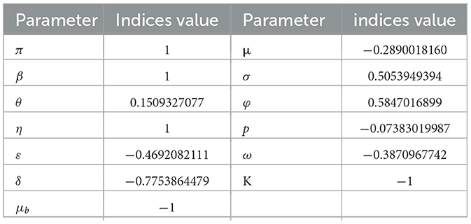
Table 2. Sensitivity indices of parameter values.

According to Table 2, the parameters with positive indices (β, θ, σ, ϕ, η, and π) show that, as their values rise, so does the effective reproduction number. If their values are raised, it suggests that they influence the spread of the disease within the population. Furthermore, as their values rise, the factors with negative sensitivity indices (ε, ω, μ, δ, μ_b, K, and p) have an impact on the effective reproduction number, which will lower the endemicity of the bacteria in the population. Figure 2 shows the reproduction number's sensitivity indices in relation to the basic parameters.

Figure 2

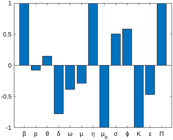
Figure 2. The local elasticity indices of R_Eff with respect to parameters of the model (1).

4 Numerical simulation

To show the analytical findings for the proposed model, we conducted a numerical computation [19, 27]. This is carried out using a set of parameter values that are listed in the table below and that in particular come from the literature, together with certain parameter considerations. The Runge-Kutta method of order four was used to execute numerical simulations of the model using the built-in MAPLE function ode45. We considered different initial conditions for the human and bacteria population. The following initial conditions, S(0) = 10, 000 I(0) = 100 V(0) = 0 R(0) = 0 B(0) = 10, with parameters in Table 1 are used for simulation.

4.1 Representation of the model when R_Eff <1 and R_Eff>1

Figure 3a demonstrates the dynamical behavior of bacteria in the environment and susceptible, vaccinated, infected, and recovered subpopulations. Additionally, the period is assumed to be between 0 and 10 months, and the initial population size for the compartmental population susceptible, vaccinated, infected, recovered, and bacteria in the environment is assumed to be respectively 10,000, 100, 0, 0, and 100. The numerical solution is convergent to the DFE point E⁰. It indicates that there are no bacteria in the environment or infected individuals for a long time and shows that there is a disease-free state that is R_Eff <1.

Figure 3

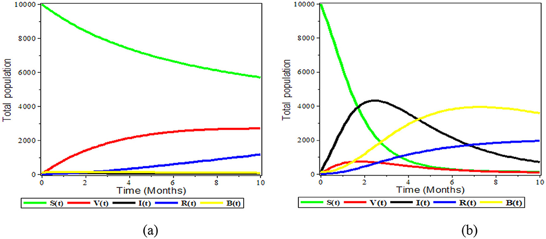
Figure 3. Graphical representation of the model (1) (a) left R_Eff < 1 and (b) right R_Eff > 1.

The susceptible and vaccinated populations decline while the number of infected grows, as can be seen in Figure 3b above. Furthermore, the infected population is entirely above the vaccinated compartment graph and, as time passes, the vaccinated compartment graph approaches the time axis graph. This suggests that the vaccinated population is close to zero and demonstrates the inefficiency of the vaccination. We observed that the disease is endemic when R_Eff is greater than one.

4.2 The effect of varying δ and φ on the population

Figures 4a–d above illustrates the impact of a combined effect of vaccination rate and vaccine efficiency. One can observe from Figure 4a that these combined effects allow reducing the size of infected individuals, and Figure 4b shows the S. typhi bacteria population as the number of vaccinations increases and its effectiveness become perfect. On the other side, the Figure 4c vaccine population and Figure 4d recovered population grow in number as the number of vaccinations increases and its effectiveness become perfect. Thus, a simultaneous increase of the effective vaccination rate and vaccine efficiency greatly reduced the proportion of the infected population. Therefore, boosting and improving the immunization rate as well as increasing the vaccine efficacy is an effective control measure against typhoid.

Figure 4

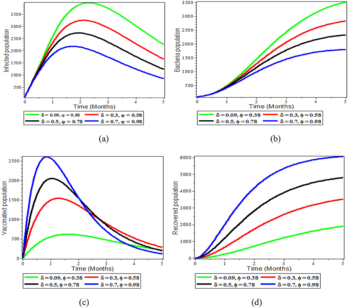
Figure 4. Graphs showing the sensitivity of model (1) varying δ and φ; (a) Infected population; (b) Bacteria population; (c) Vaccinated population; (d) Recovered population.

4.3 The effect of varying β infected population

The ingestion rate of S. typhi bacterium population is directly correlated with the disease transmission rate, as shown in Figures 5a–d below. Figures 5a, b demonstrate that, as the ingestion rate mechanisms increases, both the bacterial and infected populations increase.

Figure 5

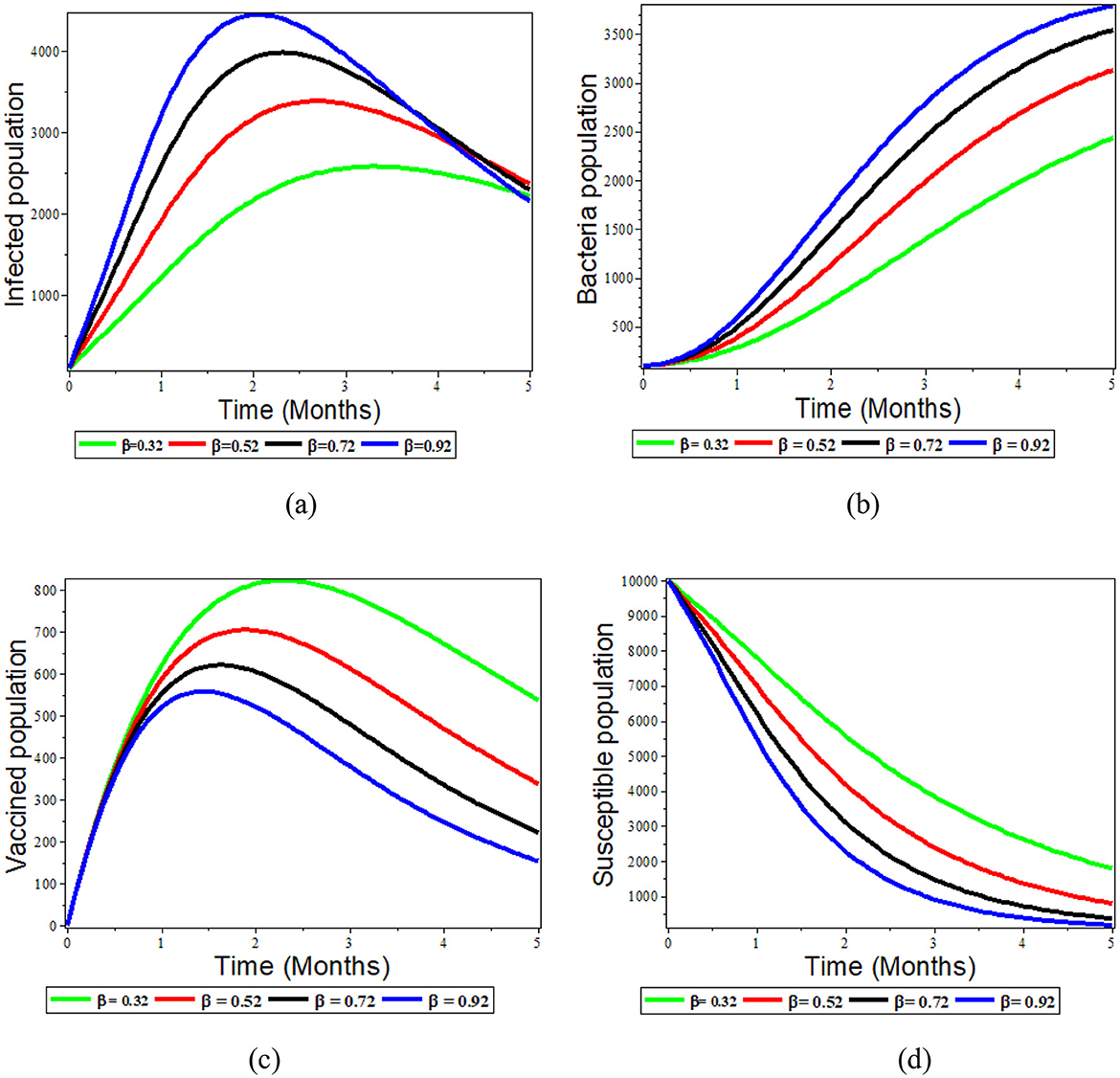
Figure 5. Graphs showing the effect of varying β on the population; (a) Infected population; (b) Bacteria population; (c) Vaccinated population; (d) Susceptible population.

Although the rate of disease transmission is inversely proportional to the number of susceptible, recovered, and vaccinated individuals, Figures 5c, d demonstrate that when the rate of ingestion increases, the number of susceptible and vaccinated individuals decreases. Therefore, ingestion rates are thus reduced when efforts are made to expand access to clean water and proper sanitation and hygiene for food handlers.

4.5 The effect of varying η on bacteria population

In this section, we illustrated the effect of varying the parameter value of η while the other parameters are fixed. From Figure 6a, the number of bacteria increases as the infectious individuals increase, contaminating the environment with S. typhi. This again leads to an increase in the number of infected people, as is shown in Figure 6b. Conversely, from Figure 6c, increasing the value of η brings a decrease in the number of susceptible people due to the increment infectious individuals and S. typhi population. The vaccine population also moves down, as is seen in the Figure 6d. Therefore, we recommend working on strategies to reduce the number of infections contaminating the environment with S. typhi. such as avoiding raw fruit and vegetables, peeling fruit yourself, and not eating the peel.

Figure 6

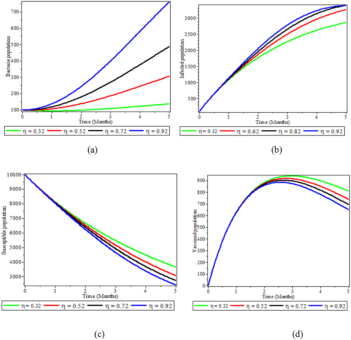
Figure 6. Graphs showing the effect of varying η on bacteria population; (a) Bacteria population; (b) Infected population; (c) Susceptible population; (d) Vaccinated population.

4.6 The effect of varying ε on bacteria population

As illustrated in Figures 7a–c, we demonstrated how the recovery of infected individuals affects the populations of bacteria, infected people, and recovered people. When we treat individuals with infections at higher rates with antibiotics and fluids, the number of infectious individuals decreases, as shown in Figure 7a. This leads to an increased number of recovered individuals, as depicted in Figure 7b. As Figure 7c also demonstrates, an increase of treatment to infectious individuals produces a reduction in the number of S. typhi bacteria population in the environment. Therefore, treatment of infected individuals is a good strategy that significantly affects bacteria concentration reduction in the environment.

Figure 7

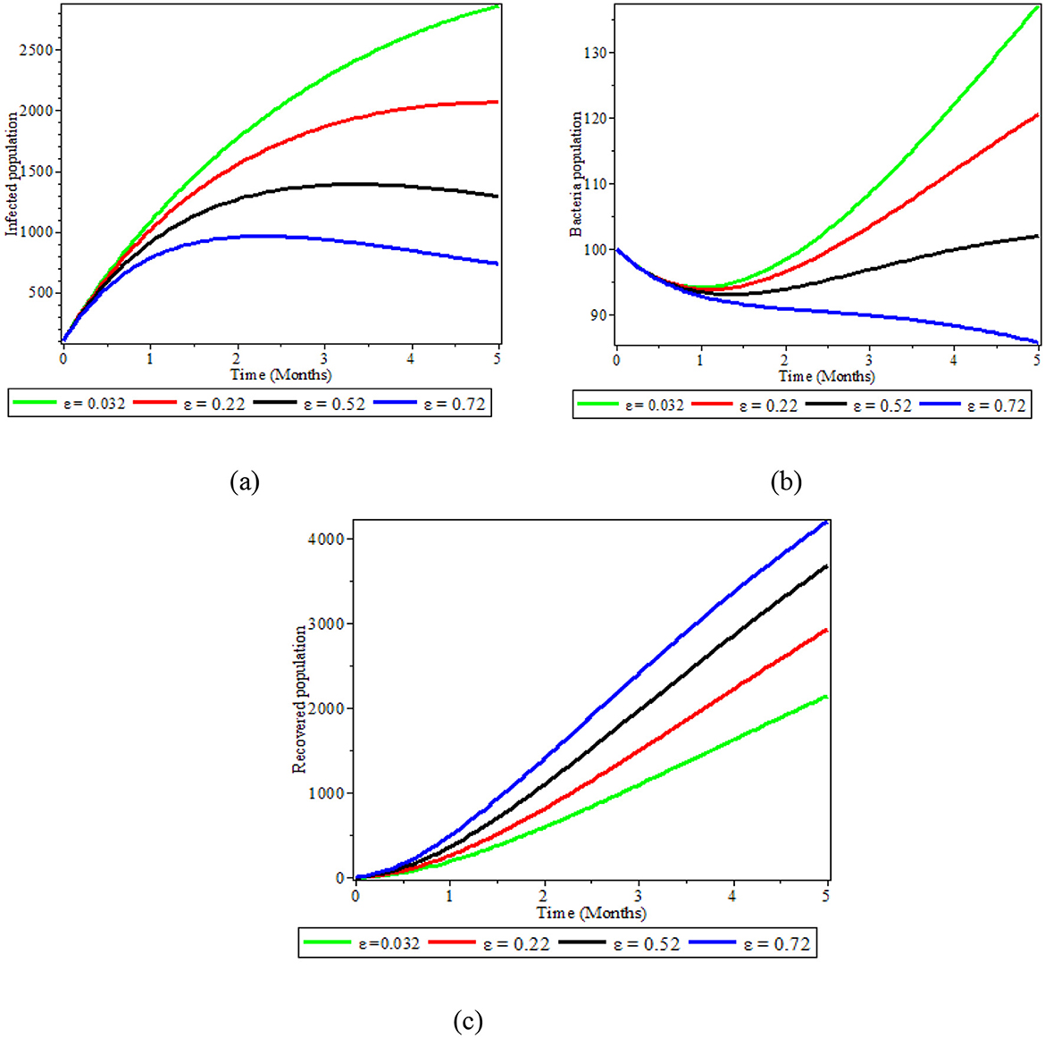
Figure 7. Graphs showing the effect of varying ε on populations; (a) Infected population; (b) Bacteria population; (c) Recovered population.

4.7 The effect of immunization on human and bacteria population

Figures 8a, b illustrates the significance of immunization in the population. As illustrated in Figure 8a, the deficiency of vaccination in the population increases the number of infected people and puts the susceptible population at risk of infection; the number of infected individuals drastically drops after the vaccination is made available to the public. We can also observe from Figure 8b that the presence of immunization in the human population reduces the bacteria in the environment. Therefore, people should get vaccinated against typhoid fever before visiting a high-risk area. However, one should still use caution when eating, drinking, and interacting with others because the typhoid vaccine is only 50–80% effective.

Figure 8

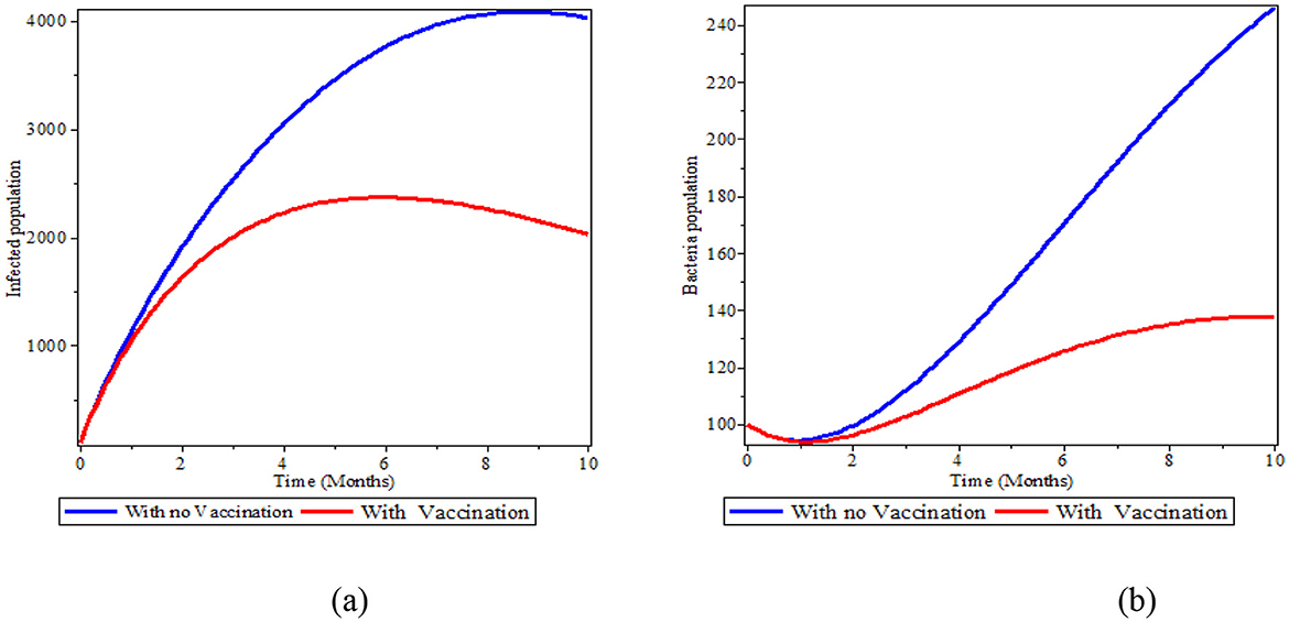
Figure 8. The effect of immunization in the infected human and bacteria population; (a) Infected population; (b) Bacteria population.

The correlation between the R_eff and β, ε, δ, φ, and η is depicted in Figures 9a–d. Figure 9a illustrates how the vaccination approaches can affect the likelihood of disease transmission within a community. Working on decreasing transmission rate below 0.2 and increasing the immunity label of susceptible individuals above 0.2 decreases the R_eff below 20%. Therefore, boosting the vaccination susceptible individuals at a higher rate dramatically lowers R_eff, which in turn lowers the probability of an outbreak.

Figure 9

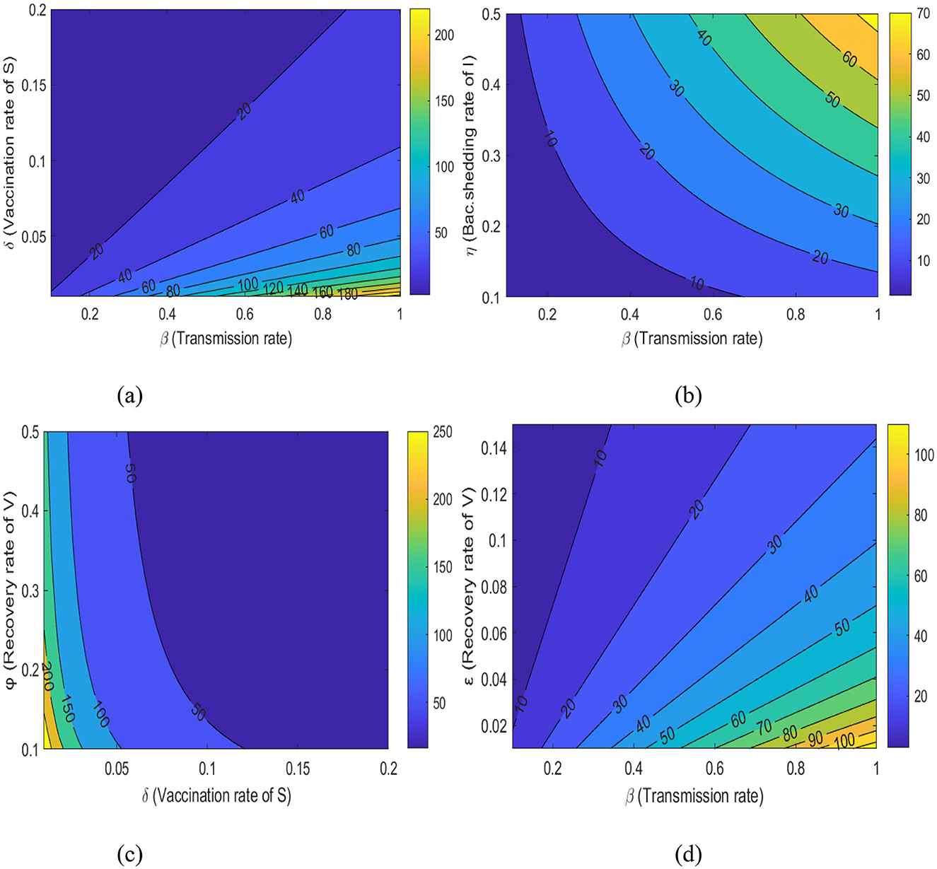
Figure 9. A contour plot illustrates the relationship between (a) R_eff with β and δ, (b) R_eff with β and η, (c) R_eff with δ and ϕ, and (d) R_eff with β and ε.

Figure 9b illustrates how variations in the shedding rate of environmental bacteria by infected individuals affects the likelihood of disease transmission within a community. If the disease transmission rate decreased below 0.4 and the shading rate increased above 0.5, R_eff can be reduced below 10%. Therefore, implementing interventions targeting sanitary deficiencies and promoting hygienic practices in the community can lower R_eff, which in turn reduces the probability of disease persistence.

Figure 9c also illustrates how the immunity rate of susceptible individuals, and consequently the recovery rate of vaccinated individuals, affects the probability of disease transmission within a community.

Boosting disease vaccination rates above 0.15 and increasing the recovery rate of vaccinated individuals above 0.15 decreases the R_eff below 50%. Finally, Figure 9d shows that increasing the recovery rate of vaccinated individuals above 0.15 and reducing the disease transmission rate below 0.2 reduces the R_eff below 20%. Therefore, we should work on interventions in the community to lesser R_eff, which in turn lowers the probability of an outbreak of the disease.

5 Results and conclusion

In this work, we studied the dynamics of typhoid fever transmission by taking into consideration S. typhi bacteria population in the environment and dividing the people into four subpopulations. After exploring a few mathematical ideas, including boundedness and equilibrium investigation, we estimated the effective reproduction number using the next-generation matrix. Moreover, we evaluated stability and confirmed that the proposed model is asymptotically stable both locally and globally for both typhoid fever-free equilibrium and endemic equilibrium points. The sensitivity analysis and numerical simulation were presented to show the practical significance of the parameters in the proposed typhoid model. By modifying the model's parameter values, a simulation study and evaluation are carried out. The pictorial representation shows that when the rates of β and η increase, the diseases propagate in the community. On the other side, as the values of the parameters ε and δ increase, the disease's ability to replicate diminishes. Typhoid vaccination rates have a substantial effect on the rate of disease transmission. Therefore, improving immunization initiatives is vital for controlling the transmission dynamics of typhoid fever. Additionally, proper disposal of feces and urine should be encouraged, and drinking water from domestic sources should be boiled or disinfected to eliminate bacteria. Additionally, it is strongly suggested that fruits should be washed with fresh water before consumption. Sanitation food and periodic medical exams should be required.

Data availability statement

The original contributions presented in the study are included in the article/supplementary material, further inquiries can be directed to the corresponding author.

Ethics statement

Ethical approval was not required for the study involving humans in accordance with the local legislation and institutional requirements. Written informed consent to participate in this study was not required from the participants or the participants' legal guardians/next of kin in accordance with the national legislation and the institutional requirements. The manuscript presents research on animals that do not require ethical approval for their study.

Author contributions

HT: Conceptualization, Supervision, Validation, Visualization, Writing – original draft. YZ: Formal analysis, Investigation, Methodology, Writing – original draft. EB: Supervision, Visualization, Writing – review & editing. GT: Conceptualization, Formal analysis, Investigation, Supervision, Writing – review & editing.

Funding

The author(s) declare that no financial support was received for the research and/or publication of this article.

Acknowledgments

Our sincere gratitude goes out to the reviewers of the research paper.

Conflict of interest

The authors declare that the research was conducted in the absence of any commercial or financial relationships that could be construed as a potential conflict of interest.

Generative AI statement

The author(s) declare that no Gen AI was used in the creation of this manuscript.

Publisher's note

All claims expressed in this article are solely those of the authors and do not necessarily represent those of their affiliated organizations, or those of the publisher, the editors and the reviewers. Any product that may be evaluated in this article, or claim that may be made by its manufacturer, is not guaranteed or endorsed by the publisher.

References

1. Heymann DL. Control of Communicable Diseases Manual (No. Ed. 19). American Public Health Association (2008).

Google Scholar

2. Crump JA, Luby SP, Mintz ED. The global burden of typhoid fever. Bull World Health Organ. (2004) 82:346–53.

Google Scholar

3. Mushayabasa S. A simple epidemiological model for typhoid with saturated incidence rate and treatment effect. Int J Math Comput Sci. (2013) 6:688–95. doi: 10.5281/zenodo.1088092

Crossref Full Text | Google Scholar

4. World Health Organization (WHO). Salmonella (Non-Typhoidal): World Health Organization. Geneva (2018).

Google Scholar

5. Peter OJ, Ibrahim MO, Akinduko OB, Rabiu M. Mathematical model for the control of typhoid fever. IOSR J Math. (2017) 13:60–6. doi: 10.9790/5728-1304026066

Crossref Full Text | Google Scholar

6. González-Guzmán J. An epidemiological model for direct and indirect transmission of typhoid fever. Math Biosci. (1989) 96:33–46. doi: 10.1016/0025-5564(89)90081-3

PubMed Abstract | Crossref Full Text | Google Scholar

7. Ashurst JV, Truong J, Woodbury B. Salmonella typhi. Florida, FL: StatPearls Publishing (2022).

Google Scholar

8. Choe K, Whittington D, Lauria DT. The economic benefits of surface water quality improvements in developing countries: a case study of davao, philippines. In: The Economics of Water Quality. Davao: Routledge (2019). pp. 371–89.

Google Scholar

9. Gordon MA, Graham SM, Walsh AL, Wilson L, Phiri A, Molyneux E, et al. Epidemics of invasive Salmonella enterica serovar enteritidis and S. enterica Serovar typhimurium infection associated with multidrug resistance among adults and children in Malawi. Clin Infect Dis. (2008) 46:963–9. doi: 10.1086/529146

PubMed Abstract | Crossref Full Text | Google Scholar

10. Maurice J. A first step in bringing typhoid fever out of the closet. Lancet. (2012) 379:699–700. doi: 10.1016/S0140-6736(12)60294-3

Crossref Full Text | Google Scholar

11. Chamuchi MN, Sigey JK, Okello JA, Okwoyo JM. SIICR model and simulation of the effects of carriers on the transmission dynamics of typhoid fever in kisii town kenya. SIJ Trans Comput Sci Eng Appl. (2014) 2:109–16. doi: 10.9756/SIJCSEA/V2I4/0203250101

Crossref Full Text | Google Scholar

12. Akinyi OC, Mugisha JYT, Manyonge A, Ouma C, Maseno K. A model on the impact of treating typhoid with antimalarial: dynamics of malaria concurrent and co-infection with typhoid. Int J Math Anal. (2015) 9:541–51. doi: 10.12988/ijma.2015.412403

Crossref Full Text | Google Scholar

13. Edward S, Nyerere N. Modelling typhoid fever with education, vaccination and treatment. Eng Math. (2016) 1:44–52. doi: 10.11648/j.ijtam.20160202.30

Crossref Full Text | Google Scholar

14. Karunditu JW, Kimathi G, Osman S. Mathematical modeling of typhoid fever disease incorporating unprotected humans in the spread dynamics. J Adv Math Comput Sci. (2019) 32:1–11. doi: 10.9734/jamcs/2019/v32i330144

Crossref Full Text | Google Scholar

15. Wameko M, Koya P, Wodajo A. Mathematical model for transmission dynamics of typhoid fever with optimal control strategies. Int J Indus Math. (2020) 12:28396.

Google Scholar

16. Nyaberi HO, Musaili JS. Mathematical modeling of the impact of treatment on the dynamics of typhoid. J Egypt Math Soc. (2021) 29:1–11. doi: 10.1186/s42787-021-00125-8

Crossref Full Text | Google Scholar

17. Jan R, Boulaaras S, Alnegga M, Abdullah FA. Fractional-calculus analysis of the dynamics of typhoid fever with the effect of vaccination and carriers. Int J Numer Model Electron Netw Devices Fields. (2024) 37:e3184. doi: 10.1002/jnm.3184

Crossref Full Text | Google Scholar

18. Van den Driessche P, Watmough J. Reproduction numbers and sub-threshold endemic equilibria for compartmental models of disease transmission. Math Biosci. (2002) 180:2948. doi: 10.1016/S0025-5564(02)00108-6

Crossref Full Text | Google Scholar

19. Simorangkir G, Aldila D, Rizka A, Tasman H, Nugraha ES. Mathematical model of tuberculosis considering observed treatment and vaccination interventions. J Interdiscip Math. (2021) 24:1717–37. doi: 10.1080/09720502.2021.1958515

Crossref Full Text | Google Scholar

20. Castillo-Chavez C, Song B. Dynamical models of tuberculosis and their applications. Math Biosci Eng. (2004) 1:361. doi: 10.3934/mbe.2004.1.361

PubMed Abstract | Crossref Full Text | Google Scholar

21. Alemneh HT, Alemu NY. Mathematical modeling with optimal control analysis of social media addiction. Infect Dis Model. (2021) 6:405–19. doi: 10.1016/j.idm.2021.01.011

PubMed Abstract | Crossref Full Text | Google Scholar

22. Tilahun GT, Alemneh HT. Mathematical modeling and optimal control analysis of COVID-19 in Ethiopia. J Interdiscip Math. (2021) 24:2101–20. doi: 10.1080/09720502.2021.1874086

Crossref Full Text | Google Scholar

23. La Salle JP. The Stability of Dynamical Systems. Pennsylvania: Society for Industrial and Applied Mathematics (1976). doi: 10.1137/1.9781611970432

Crossref Full Text | Google Scholar

24. Blower SM, Dowlatabadi H. Sensitivity and uncertainty analysis of complex models of disease transmission: an HIV model, as an example. International Statistical Review/Revue Internationale de Statistique. (1994) 62:229–43. doi: 10.2307/1403510

Crossref Full Text | Google Scholar

25. Nyerere N, Mpeshe SC, Edward S. Modeling the impact of screening and treatment on the dynamics of typhoid fever. World J Model Simul. (2018) 14:298–306.

Google Scholar

26. Engida HA, Theuri DM, Gathungu D, Gachohi J, Alemneh HT. A mathematical model analysis for the transmission dynamics of leptospirosis disease in human and rodent populations. Comput Math Methods Med. (2022) 2022:1806585. doi: 10.1155/2022/1806585

PubMed Abstract | Crossref Full Text | Google Scholar

27. Alemneh HT, Makinde OD, Theuri DM. Eco-epidemiological model and analysis of msv disease transmission dynamics in maize plant. Int J Math Math Sci. (2019) 24:7965232. doi: 10.1155/2019/7965232

Crossref Full Text | Google Scholar