Dynamic complexity of a delayed spatiotemporal predator-prey model

This study investigates a delayed spatiotemporal predator-prey model that incorporates key ecological mechanisms, including the Allee effect, fear-induced prey behavior, Holling type II predation with cooperative hunting, toxicity with delayed effects, and both nonlinear (for prey) and linear (for predators) fishing pressures. Using tools from the theory of partial differential equations, stability analysis, and Hopf bifurcation theory, we derive the conditions under which stable coexistence or instability emerges. Our results reveal that system stability is maintained below a critical delay threshold, beyond which oscillatory dynamics arise. In the spatial domain, diffusion can either stabilize populations or lead to heterogeneous patterns such as Turing structures and predator-prey segregation, particularly when diffusion is low and delays are significant. Numerical simulations support and illustrate the analytical findings, showing a variety of dynamic behaviors consistent with observed ecological patterns. This work highlights how the interplay between ecological processes, time delays, and spatial effects governs predator-prey dynamics and offers insights relevant to ecosystem management.

1 Introduction

The study of predator-prey interactions has long been fundamental in ecological modeling. Understanding how species coexist and how their populations fluctuate over time and space is essential for both theoretical ecology and natural resource management [1–6]. Natural ecosystems are often subject to various biological and environmental factors that influence species dynamics. In particular, resource competition [7], predation [8], fear effects [9, 10], and anthropogenic disturbances such as fishing play a major role in shaping population dynamics. Numerous studies have explored these dynamics using ordinary and partial differential equations [6, 11–14], allowing for a comprehensive representation of these complex interactions. For example, in Chakraborty et al. [15], the authors investigated a predator-prey model incorporating prey refuge and additional food sources for predators. Supplemental feeding is an effective strategy in integrated pest management and conservation programs. Their findings show that a high level of prey refuge can negate the benefits of supplemental food, making prey control difficult. However, when prey refuge is limited and predators have access to an optimal level of additional food, prey (pest) populations can be effectively regulated.

In this study, we propose a spatiotemporal predator-prey model that incorporates several key ecological factors. First, we integrate the Allee effect [16], which reflects the difficulty prey face in reproducing at low densities, when cooperation among individuals becomes insufficient. The Allee effect, represented by $F(b,N)=\frac{aN}{b+N}$, where N is the prey density and b is the density threshold below which reproduction is strongly reduced, is crucial for many animal and plant populations. This effect is particularly significant in situations where reproduction depends directly on the presence of a sufficient number of individuals [46–50].

Furthermore, the fear effect alters prey behavior in response to predator presence [14, 17, 18]. This mechanism is modeled by a scaling term $R(c,P)=\frac{1}{1+cP}$, which reduces prey activity and limits their access to resources, significantly affecting their reproduction rate. Moreover, the fear effect can amplify the Allee effect under certain conditions, thus altering the system dynamics and reducing the prey population in a more complex manner than a simple density effect. Recent studies also emphasize the combined roles of fear of predation, supplemental food availability, and selective predation in shaping ecological stability [19]. Fear can temporarily protect prey by reducing predator encounters, but simultaneously limits prey access to essential resources. Supplemental food supports predator persistence, while selective predation, where predators avoid infected prey, can significantly alter disease transmission and population dynamics in both temporal and spatial settings.

Another fundamental aspect of the model is the incorporation of a Holling type II functional response combined with cooperative predation. The Holling type II functional response describes a saturable consumption rate, reflecting a predator's physiological limitation. However, certain predator species hunt cooperatively, which enhances their efficiency when in groups. This cooperative hunting behavior is integrated into the model through a term that modifies the capture probability as a function of predator density.

Introducing toxicity [14] and its delayed effects adds another critical dimension to the model. Prey accumulates toxins that do not act immediately but instead cause delayed mortality, introducing a memory effect into the system. In contrast, predators experience the effects of toxicity instantaneously when consuming intoxicated prey. This temporal lag in toxin effects can induce instabilities and influence coexistence patterns and population regulation. In Shukla et al. [20], the authors studied the spatial dynamics of a nutrient–phytoplankton system under toxic effects and found that toxicity can lead to spatially inhomogeneous distributions, producing diverse patterns such as stripes, spots, or mixtures thereof. Their findings revealed that certain levels of toxicity could drive spatio-temporal oscillations, further emphasizing the potential for toxicity to generate complex dynamical behaviors in ecological systems.

Incorporating spatial diffusion into our predator-prey models is essential for realistically capturing the movement and distribution of biological populations. Diffusion terms model the natural tendency of individuals to migrate across space, which can interact with local dynamics to generate spatial heterogeneity. For instance, Shukla et al. [20] investigated the effects of cross-diffusion in an algal bloom model and demonstrated that spatial interactions could lead to the formation of complex patterns depending on environmental parameters. Their analysis highlights how spatial diffusion can either stabilize or destabilize homogeneous equilibria, depending on system conditions, and emphasizes the necessity of including such mechanisms in ecological models.

Finally, we account for resource exploitation through fishing. Prey are subject to a nonlinear Michaelis–Menten-type fishing pressure [21–23], which reflects capture saturation at high abundance levels. Predators, on the other hand, experience linear fishing pressure [24–26], corresponding to an extraction rate proportional to their density. These two forms of harvesting allow us to assess the effects of fisheries management on population stability and resilience to anthropogenic pressures [27–30].

The main objective of this study is to analyze the stability of the coexistence equilibrium of both species and explore the spatiotemporal dynamics of the system using advanced mathematical tools. We rely on eigenvalue analysis to identify equilibrium stability conditions, Hopf bifurcation theory [31–33] to examine the emergence of oscillatory behaviors due to time delays, and parabolic and elliptic partial differential equations to study spatial patterns emerging in population distribution. Numerical simulations are also conducted to illustrate the effects of various parameters on species coexistence and spatial population structuring.

This study makes a significant contribution to predator-prey system modeling by simultaneously incorporating multiple ecological and bioeconomic factors. The results will provide a deeper understanding of how spatial diffusion [34–36], delayed toxicity [12, 37–44]), and predator cooperation influence population stability and persistence. Furthermore, the inclusion of fishing pressure in the model makes our study particularly relevant to marine resource management policies and the conservation of exploited species. By combining theoretical analysis with numerical simulations, we aim to characterize the system's dynamic transitions and identify the conditions that promote species coexistence.

The predator-prey system studied is described by the following partial differential equations:

$\begin{array}{ll}\{\begin{array}{l}\frac{\partial N(x,t)}{\partial t}=d_1\Delta N+N\left(\frac{aN}{(b+N)(1+cP)}-d-eN\right)-\frac{(f+gP)NP}{1+h(f+gP)N}\\ -{\theta }_{1}NN(t-\tau )-\frac{q_1{E}_{1}N}{m_1{E}_1+m_{2}N},\\ \frac{\partial P(x,t)}{\partial t}=d_2\Delta P-mP+\frac{k(f+gP)NP}{1+h(f+gP)N}-{\theta }_{2}P-q_2{E}_{2}P,\\ \frac{\partial N(x,t)}{\partial \nu }=\frac{\partial P(x,t)}{\partial \nu }=0,\forall x\in \partial \Omega ,\forall t>0\\ N(x,t)=N_0(x,t)\ge 0,P(x,t)=P_0(x,t)\ge 0,\\ x\in \Omega ,t\in \left[-\tau ,0\right].\end{array}& (1)\end{array}$

Ω is a smooth and bounded open region in ℝ^N (where N ≥ 1), and ∂Ω represents its smooth boundary. The operator Δ corresponds to the Laplacian in ℝ^N. The unit outward normal vector on ∂Ω is denoted as S. The usage of homogeneous Neumann boundary conditions implies that the population under consideration cannot migrate or move across the boundaries of the given domain. Furthermore, we make the assumptions that N₀(x, t) and P₀(x, t) belong to the space C([−τ, 0], X), where X is defined by:

$X=\left\{v,w\in W^{2,2}(\Omega ):\frac{\partial v(t,x)}{\partial \nu }=\frac{\partial w(t,x)}{\partial \nu }=0,x\in \partial \Omega \right\}$

and the inner product 〈·, ·〉. For the sake of convenience, we limit our study to the one-dimensional spatial domain Ω = (0, lπ) throughout this paper. The parameters used in the model are defined in Table 1.

Table 1

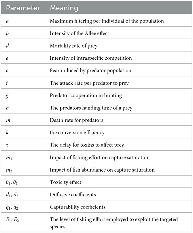
Table 1. The meaning of bioeconomical parameters.

The organization of this article is as follows. In the Section 1, we analyze the temporal model without considering the spatial dimension to better understand its intrinsic dynamics. We study the existence, positivity, and boundedness of the solutions, followed by an analysis of local stability. The Section 2 is dedicated to the study of the spatiotemporal model, where we establish the existence and boundedness of solutions, derive an a priori estimate for positive solutions, and formulate conditions for the non-existence of non-constant positive solutions. A stability analysis of the system is also conducted. In the Section 3, we examine the direction of the Hopf bifurcation and analyze the stability of the emerging periodic solutions. Finally, the Section 4 is devoted to numerical simulations, which illustrate the theoretical results on the effect of delay on stability and examine the influence of diffusion coefficients on the model's dynamics. These analyses are followed by a discussion aimed at interpreting the obtained results and highlighting their biological implications.

2 Temporal model study

We consider the following model:

$\begin{array}{ll}\{\begin{array}{l}\frac{dN}{dt}=N\left(\frac{aN}{(b+N)(1+cP)}-d-eN\right)-\frac{(f+gP)NP}{1+h(f+gP)N}\\ -{\theta }_{1}NN(t-\tau )-\frac{q_1{E}_{1}N}{m_1{E}_1+m_{2}N}\\ \frac{dP}{dt}=-mP+\frac{k(f+gP)NP}{1+h(f+gP)N}-{\theta }_{2}P-q_2{E}_{2}P\end{array}& (2)\end{array}$

With specified initial conditions x(θ) = φ(θ) > 0 and y(θ) = ψ(θ) > 0 for all θ ∈ [−τ, 0], where φ and ψ are continuous functions.

2.1 Existence, positivity, and boundedness of the solution

2.1.1 Positivity

Theorem 1. The set {(N, P) ∈ ℝ² : N ≥ 0, P ≥ 0} is positively invariant for Equation 2.

Proof. Note that the planes N = 0 and P = 0 are invariant. Indeed,

${\displaystyle \frac{\text{d}N(t)}{\text{d}t}{|}_{N=0}=0\text{and\hspace{1em}}\frac{\text{d}P(t)}{\text{d}t}{|}_{P=0}=0.}$

This means that if solutions reach N = 0 or P = 0, they do not become negative. Thus, starting with strictly positive initial conditions N(0) > 0 and P(0) > 0, solutions remain in the positive domain for all t > 0.

In conclusion, the set {(N, P) ∈ ℝ²:N ≥ 0, P ≥ 0} is positively invariant for Equation 2.

2.1.2 Boundedness

Theorem 2. All solutions of system (Equation 2), with positive initial values, are bounded.

Proof. Examine the inequality below:

$\frac{dN}{dt}\le N(a-d-eN).$

This implies that N is bounded above by $\frac{a-d}{e}$.

Now define $U=N+\frac{1}{k}P$ where k is a positive constant, and let Φ be a positive constant. We get:

$\frac{dU}{dt}+\Phi U=\frac{dN}{dt}+\frac{1}{k}\frac{dP}{dt}+\Phi U.$

Substituting the system's equations yields:

$\begin{array}{l}\frac{dU}{dt}+\Phi U=N\left(\frac{aN}{(b+N)(1+cP)}-d-eN\right)-\frac{(f+gP)NP}{1+h(f+gP)N}\\ -{\theta }_{1}NN(t-\tau )-\frac{q_1{E}_{1}N}{m_1{E}_1+m_{2}N}\\ +\frac{1}{k}(-mP+\frac{k(f+gP)NP}{1+h(f+gP)N}\\ -{\theta }_{2}P-q_2{E}_{2}P)+\Phi \left(N+\frac{1}{k}P\right).\end{array}$

Simplify this expression to get:

$\frac{dU}{dt}+\Phi U\le aN+(\Phi -d)N+\frac{1}{k}(\Phi -m)P.$

Using the bound $N\le \frac{a-d}{e}$, we obtain:

$\frac{dU}{dt}+\Phi U\le \frac{a(a-d)}{e}+(\Phi -d)N+\frac{1}{k}(\Phi -m)P.$

By choosing Φ ≤ min{d, m}, we have:

$\frac{dU}{dt}+\Phi U\le \omega =\frac{a(a-d)}{e}.$

Thus, the inequality becomes:

$U(t)\le \frac{\omega }{\Phi }+U(t_0)e^{-\Phi (t-t_0)}.$

Therefore,

$lim{\displaystyle \underset{t\to \infty }{sup}}U(t)\le \frac{\omega }{\Phi },$

Concluding that the solution of the system is bounded.

2.1.3 Existence and uniqueness of solution

We consider the following delayed system

$\begin{array}{ll}\dot{X}=g\left(X(t),X(t-\tau )\right),& (3)\end{array}$

where X = (N, P)^T represents the state vector, and the function g is defined as

$g=\left(\begin{array}{c}{g}_1\\ g_2\end{array}\right),$

with

$\begin{array}{l}\{\begin{array}{l}{g}_1=N\left(\frac{aN}{(b+N)(1+cP)}-d-eN\right)-\frac{(f+gP)NP}{1+h(f+gP)N}-{\theta }_{1}NN(t-\tau )\\ -\frac{q_1{E}_{1}N}{m_1{E}_1+m_{2}N}\\ g_2=-mP+\frac{k(f+gP)NP}{1+h(f+gP)N}-{\theta }_{2}P-q_2{E}_{2}P\end{array}\end{array}$

Theorem 3. Equation 2 has only one possible solution.

Proof. The function g : ℝ² × ℝ² → ℝ² is well-defined and continuous. Moreover, for each g_i (i = 1, 2), the partial derivatives exist and are assumed to be continuous and bounded. As a result, g satisfies the Lipschitz condition locally, ensuring the existence and uniqueness of a local solution X(t) according to the Cauchy-Lipschitz theorem for functional differential equations with delay [11].

2.2 Local stability

In this section, we initially identify and characterize all the equilibrium points of Equation 2, followed by an analysis of their local stability.

2.2.1 Equilibrium points

We concentrate exclusively on the dynamic study of internal equilibrium points. To find these, we need to solve the following system:

$\begin{array}{l}\{\begin{array}{l}\frac{aN}{(b+N)(1+cP)}-d-eN-\frac{(f+gP)P}{1+h(f+gP)N}-{\theta }_{1}N-\frac{q_1{E}_1}{m_1{E}_1+m_{2}N}=0\\ -m+\frac{k(f+gP)N}{1+h(f+gP)N}-{\theta }_2-q_2{E}_2=0\end{array}\end{array}$

Hence, the internal equilibrium can be expressed as E^*(N^*, P^*), where

$P^{*}=-\frac{f-\frac{1}{k{N}^{*}}(fh{N}^{*}+1)(m+{\theta }_2+E_2{q}_2)}{g-g\frac{h}{k}(m+{\theta }_2+E_2{q}_2)}=-\frac{C+L{N}^{*}}{D{N}^{*}}$

with

$\begin{array}{l}\{\begin{array}{l}L=f\left(-k+h{\theta }_2+hm+h{E}_2{q}_2\right)\\ C=m+{\theta }_2+E_2{q}_2\\ D=g\left(h{\theta }_2-k+hm+h{E}_2{q}_2\right)\end{array}\end{array}$

N^* is the solution to the proposed equation:

$\begin{array}{l}{Z}_7{N^{*}}^7+Z_6{N^{*}}^6+Z_5{N^{*}}^5+Z_4{N^{*}}^4+Z_3{N^{*}}^3+Z_2{N^{*}}^2+Z_1{N}^{*}\\ +Z_0=0\end{array}$

Where:

$\{\begin{array}{l}{Z}_7=D{A}_3{m}_2\left(-D+Lc\right)\left(e+{\theta }_1\right)\\ Z_6=Y_{13}+X_{14}\\ Z_5=Y_{21}+X_{12}+X_{13}+Y_{12}\\ Z_4=X_{11}+Y_{14}+Y_{15}+Y_{16}\\ Z_3=Y_{31}+Y_{32}+Y_{33}\\ Z_2=Y_{22}+Y_{23}\\ Z_1=C^2(Ccg\left(A_2+b{m}_2\right)-bD{A}_2\left(g+cf\right)\\ +3Lbcg{A}_2)\\ Z_0=C^{3}bcg{A}_2\end{array}$

And:

$\{\begin{array}{l}{X}_{11}=-D^2{A}_1{B}_1+L^{3}cg{A}_2+Lf{D}^2{A}_2-L^{2}gD{A}_2+Cf{D}^2{m}_2\\ X_{12}=-D^2{A}_1{A}_3-e{D}^2{A}_2{B}_1+L^{3}cg{m}_2+Lf{D}^2{m}_2\\ -L^{2}gD{m}_2\\ X_{13}=D^2(A_2{A}_3+B_1{m}_2)(a-d)+ebD{A}_3{m}_2(Lc-D)\\ X_{14}=-D^2(e{A}_2{A}_3+e{B}_1{m}_2-a{A}_3{m}_2+d{A}_3{m}_2+{\theta }_1{A}_2{A}_3)\\ Y_{12}=D(-{\theta }_{1}D{A}_2{B}_1+c{A}_2(eL{B}_1+C{A}_{3}e)+Cc{m}_2(B_{1}e\\ +d{A}_3\left)\right)+DLc{\theta }_1{B}_1(A_2+b{m}_2)+D(Cc{\theta }_1\\ +Lcd\left)\right(A_2{A}_3+B_1{m}_2)-b{D}^2(A_2{A}_3+B_1{m}_2\left)\right({\theta }_1+e)\\ Y_{13}=D(-{\theta }_{1}D{B}_1{m}_2+eCc{A}_3{m}_2+Lc(e{B}_1{m}_2+A_2{A}_{3}e)\\ +Lc{A}_3(d{m}_2+{\theta }_1{A}_2))+c{\theta }_1{m}_{2}D(C{A}_3+L{B}_1)\\ +Db{\theta }_1{A}_3{m}_2(-D+Lc)\\ Y_{14}=D(-2CL{m}_2(g+cf)+Cc{A}_1{A}_3+Lc(A_1{B}_1-Lf{A}_2)\\ +Lb{m}_2(fD-Lg))+Lbc{A}_{3}D(A_1+d{A}_2)\\ +DLcd{A}_2{B}_1+Dbe(-D{A}_2{B}_1+Cc(A_2{A}_3+B_1{m}_2\left)\right)\\ Y_{15}=D\left(A_2{B}_1\right(aD+eLbc)+Cc{A}_2(B_{1}e+d{A}_3)\\ +Ccd{m}_2(B_1+b{A}_3))+Lbc{B}_{1}D(d{m}_2+{\theta }_1{A}_2)\\ +Cbc{\theta }_{1}D(A_2{A}_3+B_1{m}_2)\\ Y_{16}=-b{D}^2{A}_3(A_1+d{A}_2)-d{D}^2{B}_1(A_2+b{m}_2)\\ +{\theta }_{1}D{A}_2{B}_1(Cc-bD)+L^{2}c{m}_2(3Cg-bfD+Lbg)\\ Y_{21}=D\left(Lc\right(A_1{A}_3-Lf{m}_2)-bdD{A}_3{m}_2+({\theta }_1\\ +e\left)\right(bc{A}_3(L{A}_2+C{m}_2)\left)\right)+LDbc{m}_2(B_{1}e+d{A}_3)\\ Y_{22}=C(bf{D}^2{A}_2-CcfD{A}_2-CbgD{m}_2+3L^{2}bcg{A}_2\\ +bcD{A}_1{B}_1)+3CDLbcg{m}_2-Cbcf{D}^2{m}_2\\ +bcd{D}^2{A}_2{B}_1\\ Y_{23}=-b{D}^2{A}_2{B}_1(a-d)-C^{2}D{A}_2(bD-cg)\\ Y_{31}=b{D}^2{A}_1{A}_2{A}_3\\ Y_{32}=b{D}^2(A_2^2{A}_3+B_1^2{m}_2)\\ Y_{33}=b{D}^2{A}_3{m}_2(a-d)\end{array}$

2.2.2 Characteristic equation

We consider the following equation:

$\begin{array}{ll}det\left(\lambda I-J-R{e}^{-\lambda \tau }\right)=0& (4)\end{array}$

where

$\begin{array}{l}J=\left(\begin{array}{cc}{J}_1& J_2\\ J_3& J_4\end{array}\right),R=\left(\begin{array}{cc}-{\theta }_1{N}^{*}& 0\\ 0& 0\end{array}\right)\end{array}$

and

$\begin{array}{l}\{\begin{array}{l}{J}_1=N^{*}a\frac{N^{*}+2b}{(Pc+1){(N+b)}^2}-d-2N^{*}e-P^{*}\frac{f+P^{*}g}{{(N^{*}fh+N^{*}{P}^{*}gh+1)}^2}\\ -{\theta }_1{N}^{*}-E_1^2{m}_1\frac{q_1}{{(N^{*}{m}_2+E_1{m}_1)}^2}\\ J_2=-N^{*2}a\frac{c}{{(P^{*}c+1)}^2(N^{*}+b)}-\frac{N^{*}}{{(N^{*}fh+N^{*}{P}^{*}gh+1)}^2}(N^{*}h{P}^2{g}^2\\ +2N^{*}h{P}^{*}fg+2P^{*}g+N^{*}h{f}^2+f)\\ J_3=\frac{k(f+P^{*}g)}{{(N^{*}fh+N^{*}{P}^{*}gh+1)}^2}{P}^{*}\\ J_4=-m+N^{*}k\frac{f+2P^{*}g+N{f}^{2}h+N{P}^2{g}^{2}h+2N^{*}Pfgh}{{(N^{*}fh+N^{*}{P}^{*}gh+1)}^2}-{\theta }_2-q_2{E}_2\end{array}\end{array}$

After simplifying Equation 5, we obtain the following equation:

$\begin{array}{ll}{\lambda }^2+{\alpha }_0\lambda +{\beta }_0+\left({\theta }_1{N}^{*}\lambda +{\gamma }_0\right)e^{-\lambda \tau }=0,& (5)\end{array}$

where

$\begin{array}{l}{\alpha }_0=-J_1-J_4,{\beta }_0=J_1{J}_4-J_2{J}_3,{\gamma }_0=-{\theta }_1{N}^{*}{J}_4.\end{array}$

2.2.3 Stability analysis without delay

By substituting τ = 0 into Equation 6, we obtain

$\begin{array}{l}{\lambda }^2+\left({\alpha }_0+{\theta }_1{N}^{*}\right)\lambda +{\beta }_0+{\gamma }_0=0.\end{array}$

Let us make the following assumptions:

• (H₀) ${\alpha }_0+{\theta }_1{N}^{*}>0$ and β₀ + γ₀ > 0

Theorem 4. If assumption (H₀) holds, then according to the Routh–Hurwitz criterion, the system is locally asymptotically stable.

2.2.4 Stability analysis with delay

When τ ≠ 0, by substituting λ = iω into Equation 6 and separating the real and imaginary parts, we obtain

$\begin{array}{ll}{\omega }^2-{\beta }_0={\theta }_1{N}^{*}\omega sin\left(\omega \tau \right)+{\gamma }_{0}cos\left(\omega \tau \right)& (6)\end{array}$

$\begin{array}{ll}{\alpha }_0\omega =-{\theta }_1{N}^{*}\omega cos\left(\omega \tau \right)+{\gamma }_{0}sin\left(\omega \tau \right),& (7)\end{array}$

which implies that

$\begin{array}{ll}{\omega }^4+\left({\alpha }_0^2-2{\beta }_0-{\left({\theta }_1{N}^{*}\right)}^2\right){\omega }^2+{\beta }_0^2-{\gamma }_0^2=0.& (8)\end{array}$

Let z = ω², then Equation 9 becomes

$\begin{array}{ll}{z}^2+\left({\alpha }_0^2-2{\beta }_0-{\left({\theta }_1{N}^{*}\right)}^2\right)z+{\beta }_0^2-{\gamma }_0^2=0.& (9)\end{array}$

Let us make the following assumptions:

• (H₁) ${\beta }_0^2-{\gamma }_0^2<0$

• (H₂) ${\beta }_0^2-{\gamma }_0^2⩾0$, ${\left({\alpha }_0^2-2{\beta }_0-{\theta }_2^2\right)}^2-4\left({\beta }_0^2-{\gamma }_0^2\right)⩾0$ and ${\alpha }_0^2-2{\beta }_0-{({\theta }_1{N}^{*})}^2<0$

• (H₃) ${\beta }_0^2-{\gamma }_0^2⩾0$, ${\left({\alpha }_0^2-2{\beta }_0-{({\theta }_1{N}^{*})}^2\right)}^2-4\left({\beta }_0^2-{\gamma }_0^2\right)⩽0$ or ${\alpha }_0^2-2{\beta }_0-{({\theta }_1{N}^{*})}^2>0$

• (H₄) ${\beta }_0^2-{\gamma }_0^2⩾0$, ${\left({\alpha }_0^2-2{\beta }_0-{({\theta }_1{N}^{*})}^2\right)}^2-4\left({\beta }_0^2-{\gamma }_0^2\right)⩾0$ and ${\alpha }_0^2-2{\beta }_0-{({\theta }_1{N}^{*})}^2>0$

Theorem 5. Suppose that the conditions (H₀) hold. If one of the conditions (H₃) or (H₄) is satisfied, then Equation 2 is locally asymptotically stable for all τ ≥ 0.

Next, we demonstrate under what conditions Equation 2 experiences a Hopf bifurcation by considering the delay τ as a bifurcation parameter. The necessary condition for a shift in stability of the interior equilibrium E^* is that the characteristic Equation 6 possesses purely imaginary roots. Thus, to derive the stability criterion, we substitute $\tau =\widehat{\tau }$ and $\omega =\widehat{\omega }$ into Equations 7 and 8, and by solving these equations for $cos(\widehat{\omega }\widehat{\tau })$ or $sin(\widehat{\omega }\widehat{\tau })$, we obtain:

${\widehat{\tau }}_n=\frac{1}{\widehat{\omega }}arccos\left[\frac{{\gamma }_0({\widehat{\omega }}^2-{\beta }_0)-{\theta }_1{N}^{*}{\alpha }_0{\widehat{\omega }}^2}{{({\theta }_1{N}^{*})}^2{\widehat{\omega }}^2+{\gamma }_0^2}\right]+\frac{2\pi n}{\widehat{\omega }},$

where n ∈ N. The transversality condition for Hopf bifurcation at $\tau =\widehat{\tau }$ is ${\left[\frac{d\mu }{d\tau }\right]}_{\tau =\widehat{\tau }}>0$. Let λ = μ + iω be the root of Equation 6 satisfying $\mu (\widehat{\tau })=0$ and $\omega (\widehat{\tau })=\widehat{\omega }$. Differentiating both sides of this equation with respect to τ, we get

$\begin{array}{l}{Q}_1{\left[\frac{d\mu }{d\tau }\right]}_{\tau =\widehat{\tau }}+Q_2{\left[\frac{d\omega }{d\tau }\right]}_{\tau =\widehat{\tau }}=M_3,\\ -Q_2{\left[\frac{d\mu }{d\tau }\right]}_{\tau =\widehat{\tau }}+Q_1{\left[\frac{d\omega }{d\tau }\right]}_{\tau =\widehat{\tau }}=M_4,\end{array}$

where

$\begin{array}{l}{Q}_1={\alpha }_0-{\gamma }_0\widehat{\tau }cos(\widehat{\omega }\tau )-{\theta }_1{N}^{*}\widehat{\tau }\widehat{\omega }sin(\widehat{\omega }\widehat{\tau })+{\theta }_1{N}^{*}cos(\widehat{\omega }\widehat{\tau })\\ Q_2=-2\widehat{\omega }-{\gamma }_0\widehat{\tau }sin(\widehat{\omega }\widehat{\tau })+{\theta }_1{N}^{*}sin(\widehat{\omega }\widehat{\tau })+{\theta }_1{N}^{*}\widehat{\omega }\widehat{\tau }cos(\widehat{\omega }\widehat{\tau })\\ Q_3={\gamma }_0\widehat{\omega }sin(\widehat{\omega }\widehat{\tau })-{\theta }_1{N}^{*}\widehat{\omega }\widehat{\tau }cos(\widehat{\omega }\widehat{\tau })\\ Q_4={\theta }_1{N}^{*}{\gamma }_0{\widehat{\omega }}^{2}sin(\widehat{\omega }\widehat{\tau })cos(\widehat{\omega }\widehat{\tau })\end{array}$

Thus,

${\left[\frac{d\mu }{d\tau }\right]}_{\tau =\widehat{\tau }}=\frac{Q_3{Q}_1-Q_4{Q}_2}{Q_1^2+Q_2^2}.$

The transversality condition ${\left[\frac{d\mu }{d\tau }\right]}_{\tau =\widehat{\tau }}>0$ for the occurrence of Hopf bifurcation at $\tau =\widehat{\tau }$ is properly satisfied as long as Q₃Q₁ − Q₄Q₂ > 0. Consequently, we obtain the following result:

Theorem 6. Suppose that condition (H₀) holds. If (H₁) or (H₂) is satisfied, then Equation 2 is locally asymptotically stable for $\tau <\widehat{\tau }$ and becomes unstable when $\tau >\widehat{\tau }$. Furthermore, when $\tau =\widehat{\tau }$, Equation 2 undergoes a Hopf bifurcation at (N^*, P^*) provided that M₃M₁ − M₄M₂ > 0.

3 Spatiotemporal model study

3.1 Existence and boundedness of the solution

Theorem 7. For Equation 1, we have the following results:

1. If N₀(x, t) ≥ 0 and P₀(x, t) ≥ 0, then Equation 1 has a unique positive solution (N(x, t), P(x, t)) for x ∈ Ω and t ∈ (0, ∞).

2. If (N(x, t), P(x, t)) is a solution of Equation 1, then

${\displaystyle \underset{t\to +\infty }{lim sup}}N(x,t)⩽\frac{a-d}{e}.$

Moreover, there exist constants C₁ and C₃ such that

$\parallel N(·,t){\parallel }_{C(\overline{\Omega })}⩽C_1\text{and\hspace{1em}}\parallel P(·,t){\parallel }_{C(\overline{\Omega })}⩽C_3.$

Proof. 1. We define

$\begin{array}{l}\begin{array}{l}\phi (N,P)=N\left(\frac{aN}{(b+N)(1+cP)}-d-eN\right)-\frac{(f+gP)NP}{1+h(f+gP)N}\\ -{\theta }_{1}NN(t-\tau )-\frac{q_1{E}_{1}N}{m_1{E}_1+m_{2}N}\\ \psi (N,P)=-mP+\frac{k(f+gP)NP}{1+h(f+gP)N}-{\theta }_{2}P-q_2{E}_{2}P\end{array}\end{array}$

then

$\begin{array}{ll}\begin{array}{l}{\phi }_P=\frac{-acN}{(b+N){(1+cP)}^2}-\frac{fN+h{f}^2{N}^2+2gNP+2hfg{N}^{2}P+f{g}^2{N}^2{P}^2}{{(1+h(f+gP)N)}^2}⩽0\\ {\psi }_N=\frac{k(f+gP)P}{{(1+h(f+gP)N)}^2}⩾0\end{array}& (10)\end{array}$

Next, the Equation 1 forms a mixed quasimonotone system in the set $\overline{R_{+}^2}=\left\{(N,P)/N⩾0,P⩾0\right\}$. Consider the following ordinary differential equation model:

$\begin{array}{ll}\{\begin{array}{l}\dot{N}(t)=N\left(\frac{aN}{(b+N)(1+cP)}-d-eN\right)-{\theta }_{1}NN(t-\tau )\\ -\frac{q_1{E}_{1}N}{m_1{E}_1+m_{2}N},\\ \dot{P}(t)=-mP+\frac{k(f+gP)NP}{1+h(f+gP)N}-{\theta }_{2}P-q_2{E}_{2}P,\\ N(t)=\overline{N_0},P(t)=\overline{P_0}.t\in [-\tau ,0]\end{array}& (11)\end{array}$

Where $\overline{N_0}={sup}_{\overline{\Omega }}{N}_0(x,t)$ and $\overline{P_0}={sup}_{\overline{\Omega }}{P}_0(x,t)$, ∀t ∈ [−τ, 0]. Let $(\tilde{N},\tilde{P})$ be the unique solution of the Equation 11. Then (N, P) = (0, 0) and $(\overline{N},\overline{P})=(\tilde{N},\tilde{P})$, are respectively the lower and upper solutions of the system 1. Thus, the Equation 1 has a unique globally defined solution (N(x, t), P(x, t)), which satisfies

$\begin{array}{ll}0⩽N(x,t)⩽\tilde{N}(t),0⩽P(x,t)⩽\tilde{P}(t)& (12)\end{array}$

The strong maximum principle ensures that N(x, t) > 0 and P(x, t) > 0.

$\begin{array}{l}\begin{array}{l}\frac{\partial N(x,t)}{\partial t}-d_1\Delta N=N\left(\frac{aN}{(b+N)(1+cP)}-d-eN\right)\\ -\frac{(f+gP)NP}{1+h(f+gP)N}-{\theta }_{1}NN(t-\tau )\\ -\frac{q_1{E}_{1}N}{m_1{E}_1+m_{2}N}\\ ⩽N(a-d-eN)\end{array}\end{array}$

Thus, using the comparison principle, we obtain

$\begin{array}{l}{\displaystyle \underset{t\to +\infty }{lim sup}}{\displaystyle \underset{\overline{\Omega }}{max}}N(x,t)⩽\frac{a-d}{e}\end{array}$

The maximum principle ensures that $\parallel N(.,t){\parallel }_{C(\overline{\Omega })}⩽C_1$, ∀t ⩾ 0.

Define $n(t)={\int }_{\Omega }N(x,t)dx$ and $p(t)={\int }_{\Omega }P(x,t)dx$, then

$\begin{array}{l}\begin{array}{l}\frac{\text{d}n(t)}{\text{d}t}={\displaystyle {\int }_{\Omega }}\frac{\text{d}N(x,t)}{\text{d}t}dx\\ ={\displaystyle {\int }_{\Omega }}N\left(\frac{aN}{(b+N)(1+cP)}-d-eN-{\theta }_{1}N(t-\tau )\right)\\ -\frac{(f+gP)NP}{1+h(f+gP)N}dx\\ -{\displaystyle {\int }_{\Omega }}\frac{q_1{E}_{1}N}{m_1{E}_1+m_{2}N}dx+d_1{\displaystyle {\int }_{\Omega }}\Delta Ndx\\ ={\displaystyle {\int }_{\Omega }}N\left(\frac{aN}{(b+N)(1+cP)}-d-eN-{\theta }_{1}N(t-\tau )\right)\\ -\frac{(f+gP)NP}{1+h(f+gP)N}dx-{\displaystyle {\int }_{\Omega }}\frac{q_1{E}_{1}N}{m_1{E}_1+m_{2}N}dx\end{array}\end{array}$

And for p(t):

$\begin{array}{l}\begin{array}{l}\frac{\text{d}p(t)}{\text{d}t}={\displaystyle {\int }_{\Omega }}\frac{\text{d}P(x,t)}{\text{d}t}dx\\ =d_2{\displaystyle {\int }_{\Omega }}\Delta Pdx+{\displaystyle {\int }_{\Omega }}-mP+\frac{k(f+gP)NP}{1+h(f+gP)N}\\ -{\theta }_{2}P-q_2{E}_{2}Pdx\\ ={\displaystyle {\int }_{\Omega }}-mP+\frac{k(f+gP)NP}{1+h(f+gP)N}-{\theta }_{2}P-q_2{E}_{2}Pdx\end{array}\end{array}$

which leads to

$\begin{array}{l}\begin{array}{l}\frac{\text{d}}{\text{d}t}\left(kn+p\right)⩽-m\left(kn+p\right)+\left(a-d+mk\right)n\\ ⩽-m\left(kn+p\right)+\left(a-d+mk\right)C_1|\Omega |\end{array}\end{array}$

We have

$\begin{array}{l}\begin{array}{l}{\displaystyle {\int }_{\Omega }}P(x,t)dx⩽kn(t)+p(t)\\ ⩽(kn(0)+p(0))e^{-mt}\\ +\frac{(a-d+mk)C_1|\Omega |}{m}\left(1-e^{-mt}\right)\end{array}\end{array}$

This means that

$\begin{array}{r}\parallel P(·,t){\parallel }_{L^1(\Omega )}⩽k\parallel N_0(·){\parallel }_{L^1(\Omega )}+\parallel P_0(·){\parallel }_{L^1(\Omega )}\\ +\frac{(a-d+mk)C_1|\Omega |}{m}:=C.\end{array}$

According to Theorem 3.1 in Alikakos [38], we have

$\begin{array}{l}\parallel P(·,t){\parallel }_{L^{\infty }(\Omega )}⩽C_2,\end{array}$

where C₂ depends on C and $\parallel P_0(x){\parallel }_{L^{\infty }(\Omega )}$. As a result, there exists a constant C₃ such that

$\begin{array}{l}\parallel P(·,t){\parallel }_{C(\overline{\Omega })}⩽C_3.\end{array}$

3.2 A priori estimate of the positive solution

The Equation 1 reaches its corresponding steady state.

$\begin{array}{ll}\{\begin{array}{l}-d_1\Delta N=N\left(\frac{aN}{(b+N)(1+cP)}-d-eN\right)-\frac{(f+gP)NP}{1+h(f+gP)N}\\ -{\theta }_1{N}^2-\frac{q_1{E}_{1}N}{m_1{E}_1+m_{2}N},\\ -d_2\Delta P=-mP+\frac{k(f+gP)NP}{1+h(f+gP)N}-{\theta }_{2}P-q_2{E}_{2}P,\\ \frac{\partial N(x)}{\partial \nu }=\frac{\partial P(x)}{\partial \nu }=0,\forall x\in \partial \Omega .\end{array}& (13)\end{array}$

Lemma 1. [39] We suppose that $F(x,w)\in C(\bar{\Omega }\times R)$. If $w\in C^2(\Omega )\cap C^1(\bar{\Omega })$ satisfies

$\{\begin{array}{l}\Delta w(x)+F(x,w(x))\ge 0,x\in \Omega ,\\ \frac{\partial w}{\partial \nu }\le 0,x\in \partial \Omega \end{array}$

and $w(x_0)={max}_{\bar{\Omega }}w$, then F(x₀, w(x₀)) ≥ 0. Similarly, if the two inequalities are reversed and $w(x_0)={min}_{\bar{\Omega }}w$, then F(x₀, w(x₀)) ≤ 0.

Theorem 8. Let (N(x), P(x)) be non-negative and nontrivial solution of Equation 13, then it satisfies the following conditions

$\begin{array}{l}0<N(x)⩽(a-d)/(e+{\theta }_1),0<P(x)⩽\frac{k{d}_2{\left(a-d+\frac{m{d}_1}{d_2}\right)}^2}{4d_{2}m(e+{\theta }_1)}\end{array}$

Proof. Suppose that (N(x), P(x)) is a solution of Equation 13 satisfying N(x), P(x) ⩾ 0. According to the strong maximum principle, we have N(x) > 0 and P(x) > 0. From Lemma 1, we obtain that N(x, t) ⩽ (a − d)/(e + θ₁). Multiplying the first equation of 13 by k and adding it to the second equation of 13, we obtain

$\begin{array}{l}\begin{array}{l}-\left(k{d}_1\Delta N+d_2\Delta P\right)⩽kN\left(a-d-(e+{\theta }_1)N\right)+\frac{mk{d}_1}{d_2}N\\ -\frac{m}{d_2}(d_{2}P+k{d}_{1}N)\\ ⩽kN\left(a-d+\frac{m{d}_1}{d_2}-(e+{\theta }_2)N\right)\\ -\frac{m}{d_2}(d_{2}P+k{d}_{1}N)\\ ⩽k\frac{{\left(a-d+\frac{m{d}_1}{d_2}\right)}^2}{4(e+{\theta }_1)}-\frac{m}{d_2}(d_{2}P+k{d}_{1}N).\end{array}\end{array}$

It follows from Lemma 1 that

$\begin{array}{l}k{d}_{1}N+d_{2}P⩽\frac{k{d}_2{\left(a-d+\frac{m{d}_1}{d_2}\right)}^2}{4m(e+{\theta }_1)}.\end{array}$

Therefore,

$\begin{array}{l}P⩽\frac{k{d}_2{\left(a-d+\frac{m{d}_1}{d_2}\right)}^2}{4d_{2}m(e+{\theta }_1)}.\end{array}$

3.3 Non-existence of non-constant positive solutions

Theorem 9. For any fixed a, b, c, d, e, E₁, E₂, f, g, h, k, m, m₁, m₂, q₁, q₂, θ₁ and θ₂, there exists a positive constant d^* such that if $min\left\{d_1,d_2\right\}>d^{*}$, then Equation 13 has no nonconstant solutions.

Proof. Let (N(x), P(x)) be non-negative solution of Equation 13, We define $\bar{N}=|\Omega {|}^{-1}{\int }_{\Omega }N(x)dx$ and $\bar{P}=|\Omega {|}^{-1}{\int }_{\Omega }P(x)dx$. It's clear that $\int N-\bar{N}dx=0$ and $\int P-\bar{P}dx=0$. To facilitate the discussion, let χ(N, P) = (f + gP)NP/(1 + h(f + gP)N). According to the mean value theorem for bivariate functions, we have:

$\begin{array}{l}\chi (N,P)-\chi (\bar{N},\bar{P})={\chi }_N^{\prime }(\eta ,\zeta )(N-\bar{N})-{\chi }_P^{\prime }(\eta ,\zeta )(P-\bar{P})\end{array}$

Obviously ${\chi }_N^{\prime }<k_1$ and ${\chi }_P^{\prime }<k_2$, where

$\begin{array}{l}\begin{array}{l}{k}_1=f{C}_1+g{C}_1{C}_2,\\ k_2=f{C}_1+h{f}^2{C}_1^2+2g{C}_1{C}_2+2hfg{C}_1^2{C}_2+f{g}^2{C}_1^2{C}_2^2.\end{array}\end{array}$

By multiplying the first equation of 13 by $N-\bar{N}$ and integrating over Ω, we arrive at

$\begin{array}{l}{d}_1{\displaystyle \int |}\nabla (N-\overline{N}){|}^{2}dx⩽\rho {\displaystyle \int {(N-\overline{N})}^2}dx+(M_1^2\frac{ac}{b}+\frac{ac}{b^2}{M}_1^3\\ +k_2){\displaystyle \int \Vert N-\overline{N}\Vert }\Vert P-\overline{P}\Vert dx\\ ⩽\left(\rho +M_1^2\frac{ac}{2b}+\frac{ac}{2b^2}{M}_1^3+\frac{k_2}{2}\right)\int (N\\ -\overline{N}{)}^{2}dx+\left(M_1^2\frac{ac}{2b}+\frac{ac}{2b^2}{M}_1^3+\frac{k_2}{2}\right)\\ {\displaystyle \int {(P-\overline{P})}^2}dx\end{array}$

Where

$\begin{array}{l}\rho =(d+2(e+{\theta }_1)M_1+\frac{2a}{b}{M}_1+\frac{2M_1{M}_{2}ac}{b}+\frac{a{M}_1^2}{b^2}\\ +\frac{ac}{b^2}{M}_1^2{M}_2+\frac{q_1}{m_1}+k_1)\end{array}$

Likewise, by multiplying the second equation of 13 by $P-\bar{P}$ and integrating, we achieve

$\begin{array}{l}{d}_2{\displaystyle \int |}\nabla (P-\overline{P}){|}^{2}dx⩽\left(m+{\theta }_2+q_2{E}_2+k·K_2\right){\displaystyle \int {(P-\overline{P})}^2}dx\\ +\left(k{k}_1\right){\displaystyle \int \Vert N-\overline{N}\Vert }\Vert P-\overline{P}\Vert dx\\ ⩽\left(m+v_2+q_2{E}_2+k{k}_2+k\frac{k_1}{2}\right)\int (P\\ -\overline{P}{)}^{2}dx+\frac{k{k}_1^2}{2}{\displaystyle \int {(N-\overline{N})}^2}dx\end{array}$

Applying the Poincaré inequality,

$\begin{array}{l}{\mu }_1{\displaystyle {\int }_{\Omega }}{(N-\bar{N})}^2\text{d}x⩽{\displaystyle {\int }_{\Omega }}|\nabla (N-\bar{N}){|}^2\text{d}x,{\mu }_1{\displaystyle {\int }_{\Omega }}{(P-\bar{P})}^2\text{d}x\\ ⩽{\displaystyle {\int }_{\Omega }}|\nabla (P-\bar{P}){|}^2\text{d}x,\end{array}$

where μ₁ is the second eigenvalue of the Laplace operator −Δ on Ω under homogeneous Neumann boundary condition.

$\begin{array}{l}{d}_1{\mu }_1{\int }_{\Omega }{(N-\bar{N})}^2\text{d}x+d_2{\mu }_1{\int }_{\Omega }{(P-\bar{P})}^2\text{d}x⩽A{\int }_{\Omega }{(N-\bar{N})}^2\text{d}x\\ +B{\int }_{\Omega }{(P-\bar{P})}^2\text{d}x\end{array}$

where

$\begin{array}{l}\begin{array}{l}A=\rho +M_1^2\frac{ac}{2b}+\frac{ac}{2b^2}{M}_1^3+\frac{k_2}{2}+\frac{k{k}_1^2}{2}\\ B=M_1^2\frac{ac}{2b}+\frac{ac}{2b^2}{M}_1^3+\frac{k_2}{2}+m+v_2+q_2{E}_2+k{k}_2+k\frac{k_1}{2}\end{array}\end{array}$

This implies that if

$\begin{array}{l}min\left\{d_1,d_2\right\}>d^{*}=\frac{1}{{\mu }_1}max\left\{A,B\right\},\end{array}$

then we can conclude that $\nabla (N-\bar{N})=\nabla (P-\bar{P})=0$.

3.4 Stability analysis

Characteristic equation

We consider the following equation:

$det(\lambda I-D_n-J-R{e}^{-\lambda \tau })=0$

where

$I=\left(\begin{array}{ll}1& 0\\ 0& 1\end{array}\right),\text{and\hspace{1em}}{D}_n=-\frac{n^2}{l^2}\left(\begin{array}{ll}{d}_1& 0\\ 0& d_2\end{array}\right).$

By solving the previous equation, we obtain the characteristic equation corresponding to the Equation 1

$\begin{array}{ll}{\lambda }^2+{\alpha }_n\lambda +{\beta }_n+({\theta }_1{N}^{*}\lambda +{\gamma }_n)e^{-\lambda \tau }=0,& (14)\end{array}$

where

$\begin{array}{l}{\alpha }_n=(d_1+d_2)\frac{n^2}{l^2}-(J_1+J_4),\\ {\beta }_n=d_1{d}_2\frac{n^4}{l^4}-(d_2{J}_1+d_1{J}_4)\frac{n^2}{l^2}+J_1{J}_4-J_2{J}_3,\\ {\gamma }_n={\theta }_1{N}^{*}{d}_1\frac{n^2}{l^2}-{\theta }_1{N}^{*}{J}_4.\end{array}$

Without delay

If no delay is present, the characteristic equation will take the following form:

$\begin{array}{ll}{\lambda }^2+({\alpha }_n+{\theta }_1{N}^{*})\lambda +{\beta }_n+{\gamma }_n=0,& (15)\end{array}$

We make the following assumption:

• (H₅) ${\alpha }_n+{\theta }_1{N}^{*}>0,$ β_n + γ_n > 0, for n ∈ ℕ₀,

• (H₆), ${\alpha }_0+{\theta }_1{N}^{*}>0,$ ${\alpha }_k+{\theta }_1{N}^{*}<0$, (or β_k + γ_k < 0), for some k ∈ ℕ.

Theorem 10. For the Equation 1, suppose that τ = 0. The point (N^*, P^*) is locally asymptotically stable under (H₅) and is Turing unstable under (H₆).

Proof. If (H₅) holds, we can determine that the characteristic roots of Equation 15 all have negative real parts. Hence, (N^*, P^*) is locally asymptotically stable. If (H₆) holds, then the characteristic roots for k ∈ ℕ have at least one positive real part, but with n = 0, they all have negative real parts. This implies that (N^*, P^*) is Turing unstable.

With delay

Let iω(ω > 0) be a solution of Equation 14; then,

$\begin{array}{ll}-{\omega }^2+\text{i}\omega {\alpha }_n+{\beta }_n+\left({\gamma }_n+{\theta }_1{N}^{*}\text{i}\omega \right)(cos\omega \tau -\text{i}sin\omega \tau )=0& (16)\end{array}$

We obtain:

$\begin{array}{l}cos\omega \tau =\frac{{\omega }^2({\gamma }_n-{\theta }_1{N}^{*}{\alpha }_n)-{\beta }_n{\gamma }_n}{{\gamma }_n^2+{({\theta }_1{N}^{*})}^2{\omega }^2},\end{array}$

$\begin{array}{ll}sin\omega \tau =\frac{\omega \left({\alpha }_n{\gamma }_n-{\theta }_1{N}^{*}{\beta }_n+{\theta }_1{N}^{*}{\omega }^2\right)}{{\gamma }_n^2+{({\theta }_1{N}^{*})}^2{\omega }^2}.& (17)\end{array}$

This leads to:

$\begin{array}{ll}{\omega }^4+\left({\alpha }_n^2-2{\beta }_n-{({\theta }_1{N}^{*})}^2\right){\omega }^2+{\beta }_n^2-{\gamma }_n^2=0.& (18)\end{array}$

Let z = ω²; then,

$\begin{array}{ll}{z}^2+\left({\alpha }_n^2-2{\beta }_n-{({\theta }_1{N}^{*})}^2\right)z+{\beta }_n^2-{\gamma }_n^2=0& (19)\end{array}$

and the roots of Equation 19 are

$z^{\pm }=\frac{1}{2}\left[-L_n\pm \sqrt{L_n^2-4M_n{N}_n}\right],$

where

$\begin{array}{l}{L}_n={\alpha }_n^2-2{\beta }_n-{\left({\theta }_1{N}^{*}\right)}^2,M_n={\beta }_n+{\gamma }_n,N_n={\beta }_n-{\gamma }_n.\end{array}$

If (H₅) is satisfied, M_n > 0(n ∈ ℕ₀). Define

$\begin{array}{l}{𝕎}_1=\left\{n\mid N_n<0,n\in {\mathbb{N}}_0\right\},\\ {𝕎}_2=\left\{n\mid N_n>0,L_n<0,L_n^2-4M_n{N}_n>0,n\in \mathbb{N}\right\},\\ {𝕎}_3=\left\{n\mid R_n>0,L_n^2-4M_n{N}_n<0,n\in \mathbb{N}\right\},\end{array}$

and

$\begin{array}{l}{\omega }_n^{\pm }=\sqrt{z_n^{\pm }},{\tau }_n^{j,\pm }=\{\begin{array}{ll}\frac{1}{{\omega }_n^{\pm }}arccos\left(V_{cos}^{(n,\pm )}\right)+2j\pi ,& V_{\text{sin}}^{(n,\pm )}\ge 0,\\ \frac{1}{{\omega }_n^{\pm }}\left[2\pi -arccos\left(V_{cos}^{(n,\pm )}\right)\right]\\ +2j\pi ,& V_{\text{sin}}^{(n,\pm )}<0.\end{array}\end{array}$

where

$\begin{array}{l}{V}_{cos}^{(n,\pm )}=\frac{{\left({\omega }_n^{\pm }\right)}^2({\gamma }_n-{\theta }_1{N}^{*}{\alpha }_n)-{\beta }_n{\gamma }_n}{{\gamma }_n^2+{({\theta }_1{N}^{*})}^2{\left({\omega }_n^{\pm }\right)}^2},\\ V_{sin}^{(n,\pm )}=\frac{{\omega }_n^{\pm }\left({\alpha }_n{\gamma }_n-{\theta }_1{N}^{*}{\beta }_n+{\theta }_1{N}^{*}{\left({\omega }_n^{\pm }\right)}^2\right)}{{\gamma }_n^2+{({\theta }_1{N}^{*})}^2{\left({\omega }_n^{\pm }\right)}^2}.\end{array}$

Lemma 2. Assuming that (H₅) is satisfied, the following results hold:

• The Equation 14 has a pair of purely imaginary roots $\pm i{\omega }_n^{+}$ at ${\tau }_n^{j,+}$ for j ∈ ℕ₀ and n ∈ 𝕎₁.

• The Equation 14 has two pairs of purely imaginary roots $\pm i{\omega }_n^{\pm }$ at ${\tau }_n^{j,\pm }$ for j ∈ ℕ₀ and n ∈ 𝕎₂.

• The Equation 14 has no purely imaginary root for n ∈ 𝕎₃.

Lemma 3. Suppose that (H₅) is satisfied. Then, $Re\left(\frac{d\lambda }{d\tau }\right){|}_{\tau ={\tau }_n^{j,+}}>0,Re\left(\frac{d\lambda }{d\tau }\right){|}_{\tau ={\tau }_n^{j,-}}<0$ for n ∈ 𝕎₁ ∪ 𝕎₂ and j ∈ ℕ₀.

Proof. From Equation 14, we have

$\begin{array}{l}{\left(\frac{d\lambda }{d\tau }\right)}^{-1}=\frac{2\lambda +{\alpha }_n+{\theta }_1{N}^{*}{e}^{-\lambda \tau }}{({\gamma }_n+{\theta }_1{N}^{*}\lambda )\lambda e^{-\lambda \tau }}-\frac{\tau }{\lambda }.\end{array}$

Thus,

$\begin{array}{l}{\left[\mathrm{Re}{\left(\frac{d\lambda }{d\tau }\right)}^{-1}\right]}_{\tau ={\tau }_n^{j,\pm }}=\mathrm{Re}{\left[\frac{2\lambda +{\alpha }_n+{\theta }_1{N}^{*}{e}^{-\lambda \tau }}{\left({\gamma }_n+{\theta }_1{N}^{*}\lambda \right)\lambda e^{-\lambda \tau }}-\frac{\tau }{\lambda }\right]}_{\tau ={\tau }_n^{j,\pm }}\\ =[\frac{1}{{\gamma }_n^2+{\left({\theta }_1{N}^{*}\right)}^2{\omega }^2}(2{\omega }^2+{\alpha }_n^2-2{\beta }_n\\ {-{\left({\theta }_1{N}^{*}\right)}^2)]}_{\tau ={\tau }_n^{j,\pm }}\\ =\pm [\frac{1}{{\gamma }_n^2+{\left({\theta }_1{N}^{*}\right)}^2{\omega }^2}\\ {\sqrt{{\left({\alpha }_n^2-2{\beta }_n-{\left({\theta }_1{N}^{*}\right)}^2\right)}^2-4\left({\beta }_n^2-{\gamma }_n^2\right)}]}_{\tau ={\tau }_n^{j,\pm }}.\end{array}$

Therefore, $Re\left(\frac{d\lambda }{d\tau }\right){|}_{\tau ={\tau }_n^{j,+}}>0$, and $Re\left(\frac{d\lambda }{d\tau }\right){|}_{\tau ={\tau }_n^{j,-}}<0$.

Let ${\tau }_{*}=min\left\{{\tau }_n^0\mid n\in {𝕎}_1\cup {𝕎}_2\right\}$. We have the following theorem:

Theorem 11. Suppose that (H₅) is satisfied. Then, the following results hold:

• The positive equilibrium (N^*, P^*) of the Equation 2 is asymptotically stable for τ ∈ [0, τ_*).

• The Equation 2 undergoes a Hopf bifurcation at the positive equilibrium (N^*, P^*) when $\tau ={\tau }_n^{j,\pm }$ for n ∈ 𝕎₁ ∪ 𝕎₂ and j ∈ ℕ₀.

4 Hopf bifurcation

In this section, our goal is to obtain the normal form of Hopf bifurcation at the interior equilibrium. Let $\bar{N}(x,t)=N(x,\tau t)-N^{*}$ and $\bar{P}(x,t)=P(x,\tau t)-P^{*}$. In this context, we've omitted the bar for simplicity. Thus, the resulting system is as follows

$\{\begin{array}{l}\frac{\partial N(x,t)}{\partial t}=\tau [d_1\Delta N+(N+N^{*})\\ \left(\frac{a(N+N^{*})}{(b+N+N^{*})(1+c(P+P^{*}))}-d-e(N+N^{*})\right)\\ -{\theta }_1(N+N^{*})(N(t-1)+N^{*})\\ -\frac{(f+g(P+P^{*}))(N+N^{*})(P+P^{*})}{1+h(f+g(P+P^{*}))(N+N^{*})}\\ -\frac{q_1{E}_1(N+N^{*})}{m_1{E}_1+m_2(N+N^{*})}],\\ \frac{\partial P(x,t)}{\partial t}=\tau [d_2\Delta P-(m+{\theta }_2+q_2{E}_2)(P+P^{*})\\ +\frac{k(f+g(P+P^{*}))(N+N^{*})(P+P^{*})}{1+h(f+g(P+P^{*}))(N+N^{*})}]\end{array}$

Denote $\tau =\tilde{\tau }+\epsilon$, and U = (N(x, t), P(x, t))^T. In the phase space C: = C([−1, 0], X) it can be reformulated as

$\frac{\text{d}U(t)}{\text{d}t}=\tilde{\tau }D\Delta U(t)+L_{\tilde{\tau }}(U_t)+F(U_t,\epsilon ),$

where

$L_{\epsilon }(\phi )=\epsilon \left(\begin{array}{c}{J}_1{\phi }_1(0)+J_2{\phi }_2(0)-{\theta }_1{N}^{*}{\phi }_1(-1)\\ J_3{\phi }_1(0)+J_4{\phi }_2(0)\end{array}\right)$

and

$F(\phi ,\epsilon )=\epsilon D\Delta \phi +L_{\epsilon }(\phi )+f(\phi ,\epsilon ),$

such that

$f(\phi ,\epsilon )=(\tilde{\tau }+\epsilon ){(f_1(\phi ,\epsilon ),f_2(\phi ,\epsilon ))}^T,$

with

$\begin{array}{l}{f}_1\left(\phi ,\epsilon \right)=\frac{a{\left({\phi }_1\left(0\right)+N^{*}\right)}^2}{\left(b+\left({\phi }_1\left(0\right)+N^{*}\right)\right)\left(1+c\left({\phi }_2\left(0\right)+P^{*}\right)\right)}\\ -d\left({\phi }_1\left(0\right)+N^{*}\right)-e{\left({\phi }_1\left(0\right)+N^{*}\right)}^2\\ -\frac{\left(f+g\left({\phi }_2\left(0\right)+P^{*}\right)\right)\left({\phi }_1\left(0\right)+N^{*}\right)\left({\phi }_2\left(0\right)+P^{*}\right)}{1+h\left(f+g\left({\phi }_2\left(0\right)+P^{*}\right)\right)\left({\phi }_1\left(0\right)+N^{*}\right)}\\ -{\theta }_1\left({\phi }_1\left(0\right)+N^{*}\right)\left({\phi }_1\left(-1\right)+N^{*}\right)\\ -\frac{q_1{E}_1\left({\phi }_1\left(0\right)+N^{*}\right)}{m_1{E}_1+m_2\left({\phi }_1\left(0\right)+N^{*}\right)}\\ f_2\left(\phi ,\epsilon \right)=-\left(m+{\theta }_2+q_2{E}_2\right)\left({\phi }_2\left(0\right)+P^{*}\right)\\ +\frac{k\left(f+g\left({\phi }_2\left(0\right)+P^{*}\right)\right)\left({\phi }_1\left(0\right)+N^{*}\right)\left({\phi }_2\left(0\right)+P^{*}\right)}{1+h\left(f+g\left({\phi }_2\left(0\right)+P^{*}\right)\right)\left({\phi }_1\left(0\right)+N^{*}\right)}\end{array}$

Respectively, for $\phi ={({\phi }_1,{\phi }_2)}^T\in C_1$. We know that ${\Lambda }_n:=\left\{i{\omega }_n\tilde{\tau },-i{\omega }_n\tilde{\tau }\right\}$ are characteristic roots of

$\frac{\text{d}z(t)}{\text{d}t}=-\tilde{\tau }D\frac{n^2}{l^2}z(t)+L_{\tilde{\tau }}(z_t)$

The application of the Riesz representation theorem allows us to establish the existence of a 2 × 2 matrix function ${\eta }^n(s,\tilde{\tau }),(-1\le s\le 0)$, whose elements are of bounded variation functions such that

$-\tilde{\tau }D\frac{n^2}{l^2}\phi (0)+L_{\tilde{\tau }}(\phi )={\displaystyle {\int }_{-1}^0}d{\eta }^n(s,\tau )\phi (s)$

for φ ∈ C([−1, 0], ℝ²). Choose

${\eta }^n(s,\tau )=\{\begin{array}{ll}\tau E& s=0\\ 0& s\in (-1,0)\\ -\tau F& s=-1\end{array}$

where

$E=\left(\begin{array}{cc}{J}_1-d_1\frac{n^2}{l^2}& J_2\\ J_3& J_4-d_2\frac{n^2}{l^2}\end{array}\right),F=\left(\begin{array}{cc}-{\theta }_1{N}^{*}& 0\\ 0& 0\end{array}\right)$

Define the bilinear paring

$\begin{array}{l}(\psi ,\phi )=\psi (0)\phi (0)-{\displaystyle {\int }_{-1}^0}{\displaystyle {\int }_{\xi =0}^s}\psi (\xi -s)d{\eta }^n(s,\tilde{\tau })\phi (\xi )d\xi \\ =\psi (0)\phi (0)+\tilde{\tau }{\displaystyle {\int }_{-1}^0}\psi (\xi +1)F\phi (\xi )d\xi .\end{array}$

for $\phi \in C([-1,0],{ℝ}^2),\psi \in C([0,1],{ℝ}^2).A(\tilde{\tau })$ has a pair of simple purely imaginary eigenvalues $\pm i{\omega }_n\tilde{\tau }$, and they are also eigenvalues of A^*. Define $p_1(\theta )={(1,\zeta )}^T{e}^{i{\omega }_n\tilde{\tau }s}(s\in [-1,0]),q_1(r)=$ $(1,\vartheta )e^{-i{\omega }_n\tilde{\tau }r}(r\in [0,1])$, where

$\begin{array}{l}\zeta =\frac{1}{J_2}\left(-J_1+d_1\frac{n^2}{l^2}+{\theta }_1{N}^{*}{e}^{-i\tilde{\tau }{\omega }_n}+i{\omega }_n\right),\\ \vartheta =\frac{1}{J_3}\left(-J_1+d_1\frac{n^2}{l^2}+{\theta }_1{N}^{*}{e}^{i\tilde{\tau }{\omega }_n}-i{\omega }_n\right),\end{array}$

Let Φ = (Φ₁, Φ₂) and ${{\rm Y}}^{*}={({{\rm Y}}_1^{*},{{\rm Y}}_2^{*})}^T$ with

$\begin{array}{l}{\Phi }_1(s)=\frac{p_1(s)+p_2(s)}{2}=\left(\begin{array}{l}Re\left(e^{i{\omega }_n\tilde{\tau }s}\right)\\ Re\left(\zeta e^{i{\omega }_n\tau s}\right)\end{array}\right),\\ {\Phi }_2(s)=\frac{p_1(s)-p_2(s)}{2i}=\left(\begin{array}{l}Im\left(e^{i{\omega }_n\tilde{\tau }s}\right)\\ Im\left(\zeta e^{i{\omega }_n\tilde{\tau }s}\right)\end{array}\right)\\ \end{array}$

for θ ∈ [−1, 0], and

$\begin{array}{l}{{\rm Y}}_1^{*}(r)=\frac{q_1(r)+q_2(r)}{2}=\left(\begin{array}{l}Re\left(e^{-i{\omega }_n\tilde{\tau }\text{r}}\right)\\ Re\left(\vartheta e^{-i{\omega }_n\tilde{\tau }r}\right)\end{array}\right),\\ {{\rm Y}}_2^{*}(r)=\frac{q_1(r)-q_2(r)}{2i}=\left(\begin{array}{l}Im\left(e^{-i{\omega }_n\tilde{\tau }r}\right)\\ Im\left(\vartheta e^{-i{\omega }_n\tilde{r}r}\right)\end{array}\right)\\ \end{array}$

for r ∈ [0, 1]. Define

$\begin{array}{l}{D}_1^{*}:=({{\rm Y}}_1^{*},{\Phi }_1),D_2^{*}:=({{\rm Y}}_1^{*},{\Phi }_2),D_3^{*}:=({{\rm Y}}_2^{*},{\Phi }_1),\\ D_4^{*}:=({{\rm Y}}_2^{*},{\Phi }_2).\end{array}$

Define $({{\rm Y}}^{*},\Phi )=\left({{\rm Y}}_j^{*},{\Phi }_k\right)=\left(\begin{array}{ll}{D}_1^{*}& D_2^{*}\\ D_3^2& D_4^{*}\end{array}\right)$ and construct a new basis ϒ for P^* by

${\rm Y}={({{\rm Y}}_1,{{\rm Y}}_2)}^T={({{\rm Y}}^{*},\Phi )}^{-1}{{\rm Y}}^{*}\text{.}$

Then (ϒ, Φ) = I₂. In addition, define $f_n:=(f_n^1,f_n^2)$, where

$f_n^1=\left(\begin{array}{c}{\psi }_n(x)\\ 0\end{array}\right),f_n^2=\left(\begin{array}{c}0\\ {\psi }_n(x)\end{array}\right),{\psi }_n(x)=cos\left(\frac{n}{l}x\right).$

We also define

$c.f_n=c_1{f}_n^1+c_2{f}_n^2,\text{for\hspace{1em}}c={(c_1,c_2)}^T\in C_1$

and

$\begin{array}{r}<u,v>:=\frac{1}{l\pi }{\displaystyle {\int }_0^{l\pi }}{u}_1\overline{v_1}dx+\frac{1}{l\pi }{\displaystyle {\int }_0^{l\pi }}{u}_2\overline{v_2}dx\\ \text{for}u=(u_1,u_2),v=(v_1,v_2),u,v\in X\end{array}$

and

$\langle \phi ,f_0\rangle ={\left(<\phi ,f_0^1>,<\phi ,f_0^2>\right)}^T$

Rewrite Equation 1 as the following abstract form

$\frac{\text{d}U(t)}{\text{d}t}=A_{\tilde{\tau }}{U}_t+R(U_t,\epsilon ),$

where

$R(U_t,\epsilon )=\{\begin{array}{ll}0,& \theta \in [-1,0)\\ F(U_t,\epsilon ),& \theta =0\end{array}$

The solution is

$U_t=\Phi \left(\begin{array}{l}{x}_1\\ x_2\end{array}\right)f_n+h(x_1,x_2,\epsilon ),$

where

$\left(\begin{array}{l}{x}_1\\ x_2\end{array}\right)=\left({\rm Y},<U_t,f_n>\right),$

and

$h(x_1,x_2,\epsilon )\in P_S{C}_1,h(0,0,0)=0,Dh(0,0,0)=0$

Then

$U_t=\Phi \left(\begin{array}{l}{x}_1(t)\\ x_2(t)\end{array}\right)f_n+h(x_1,x_2,0)$

Let z = x₁ − ix₂, and notice that p₁ = Φ₁ + iΦ₂. Then

$\Phi \left(\begin{array}{l}{x}_1\\ x_2\end{array}\right)f_n=({\Phi }_1,{\Phi }_2)\left(\begin{array}{c}\frac{z+\bar{z}}{2}\\ \frac{i(z-\bar{z})}{2}\end{array}\right)f_n=\frac{1}{2}(p_{1}z+\overline{p_{1}z})f_n$

and $h(x_1,x_2,0)=h\left(\frac{z+\bar{z}}{2},\frac{i(z-\bar{z})}{2},0\right)$. Then

$\begin{array}{l}{U}_t=\frac{1}{2}(p_{1}z+\overline{p_{1}z})f_n+h\left(\frac{z+\bar{z}}{2},\frac{i(z-\bar{z})}{2},0\right)\\ =\frac{1}{2}(p_{1}z+\overline{p_{1}z})f_n+W(z,\bar{z}),\end{array}$

where $W(z,\bar{z})=h\left(\frac{z+\bar{z}}{2},\frac{i(z-\bar{z})}{2},0\right)$, and $ż=i{\omega }_n\tilde{\tau }z+g(z,\bar{z}),$ where

$g(z,\bar{z})=\left({{\rm Y}}_1(0)-i{{\rm Y}}_2(0)\right)<F(U_t,0),f_n>$

Let

$\begin{array}{l}W(z,\bar{z})=W_{20}\frac{z^2}{2}+W_{11}z\bar{z}+W_{02}\frac{{\bar{z}}^2}{2}+\cdots ,\\ g(z,\bar{z})=g_{20}\frac{z^2}{2}+g_{11}z\bar{z}+g_{02}\frac{{\bar{z}}^2}{2}+\cdots ,\end{array}$

then

$\begin{array}{l}{u}_t(0)=\frac{1}{2}(z+\bar{z}){\psi }_n(x)+W_{20}^{(1)}(0)\frac{z^2}{2}+W_{11}^{(1)}(0)z\bar{z}+W_{02}^{(1)}(0)\frac{{\bar{z}}^2}{2}\\ +\cdots ,\\ v_t(0)=\frac{1}{2}(\zeta z+\bar{\zeta }\bar{z}){\psi }_n(x)+W_{20}^{(2)}(0)\frac{z^2}{2}+W_{11}^{(2)}(0)z\bar{z}\\ +W_{02}^{(2)}(0)\frac{{\bar{z}}^2}{2}+\cdots ,\\ u_t(-1)=\frac{1}{2}\left(z{e}^{-i{\omega }_n\tilde{\tau }}+\bar{z}{e}^{i{\omega }_n\tilde{\tau }}\right){\psi }_n(x)+W_{20}^{(1)}(-1)\frac{z^2}{2}\\ +W_{11}^{(1)}(-1)z\bar{z}+W_{02}^{(1)}(-1)\frac{{\bar{z}}^2}{2}+\cdots \end{array}$

and

$\begin{array}{l}{\bar{F}}_1(U_t,0)=\frac{1}{\tilde{\tau }}{F}_1=a_{20}{u}_t^2(0)+a_{11}{u}_t(0)v_t(0)+a_{02}{v}_t^2(0)\\ +a_{30}{u}_t^3(0)+a_{21}{u}_t^2(0)v_t(0)+a_{12}{u}_t(0)v_t^2(0)\\ +a_{03}{v}_t^3(0)+c_{20}{u}_t^2(-1)+\cdots ,\\ {\bar{F}}_2(U_t,0)=\frac{1}{\tilde{\tau }}{F}_2=b_{20}{u}_t^2(0)+b_{11}{u}_t(0)v_t(0)+b_{02}{v}_t^2(0)\\ +b_{30}{u}_t^3(0)+b_{21}{u}_t^2(0)v_t(0)+b_{12}{u}_t(0)v_t^2(0)\\ +b_{03}{v}_t^3(0)+\cdots \end{array}$

Where

$\begin{array}{l}{a}_{20}=\frac{a{b}^2}{(1+c{P}^{*}){(b+N^{*})}^3}-e+\frac{h{P}^{*}{(f+g{P}^{*})}^2}{{(1+h(f+g{P}^{*})N^{*})}^3}\\ +\frac{q_1{m}_1{m}_2{E}_1^2}{{(m_1{E}_1+m_2{N}^{*})}^3},\\ b_{20}=-k\frac{\mathrm{hv}{(f+g{P}^{*})}^2}{{(1+h(f+g{P}^{*})N^{*})}^3},a_{11}=\frac{-ac({(N^{*})}^2+2b{N}^{*})}{{(b+N^{*})}^2{(1+c{P}^{*})}^2}\\ -\frac{1}{k}{b}_{11},\\ b_{11}=\frac{k(f+h{f}^2{N}^{*}+hfg{N}^{*}{P}^{*}+2g{P}^{*})}{{(1+h(f+g{P}^{*})N^{*})}^3},\\ b_{30}=k\frac{h^2{P}^{*}{(f+g{P}^{*})}^3}{{(1+h(f+g{P}^{*})N^{*})}^4},\\ a_{30}=\frac{-a{b}^2}{{(1+c{P}^{*})}^2{(b+N^{*})}^4}-\frac{h^2{P}^{*}{(f+g{P}^{*})}^3}{{(1+h(f+g{P}^{*})N^{*})}^4}\\ -\frac{q_1{m}_1{m}_2^2{E}_1^2}{{(m_1{E}_1+m_2{N}^{*})}^4},\\ b_{21}=\frac{\begin{array}{c}-k(h{f}^2+h^2{f}^2{N}^{*}+2h^2{b}^{2}g{N}^{*}{P}^{*}+4hfg{P}^{*}\\ +h^{2}f{g}^2{N}^{*}{(P^{*})}^2+3h{g}^2{(P^{*})}^2)\end{array}}{{(1+hf{N}^{*}+hg{N}^{*}{P}^{*})}^4},\\ a_{21}=\frac{-ac{b}^2}{{(1+c{P}^{*})}^2{(b+N^{*})}^3}-\frac{1}{k}{b}_{21},\\ b_{02}=kg{N}^{*}\frac{1+hb{N}^{*}}{{(1+hb{N}^{*}+hg{N}^{*}{P}^{*})}^3},\\ b_{03}=-6kh{g}^2{(N^{*})}^2\frac{1+h{f}_N^{*}}{{(1+h{f}_N^{*}+hg{N}^{*}{P}^{*})}^4},\\ a_{02}=\frac{a{c}^2{(N^{*})}^2}{(b+N^{*}){(1+c{P}^{*})}^3}-\frac{1}{k}{b}_{02},\\ a_{03}=\frac{-a{c}^3{(N^{*})}^2}{(b+N^{*}){(1+c{P}^{*})}^4}-\frac{1}{k}{b}_{03},\\ a_{12}=\frac{a{c}^2({(N^{*})}^2+2b{N}^{*})}{{(b+N^{*})}^2{(1+c{P}^{*})}^3}-\frac{1}{k}{b}_{12},\\ b_{12}=\frac{-k(h^2{b}^{2}g{(N^{*})}^2+h^{2}b{g}^2{(N^{*})}^2{P}^{*}+2h{g}^2{N}^{*}r-g)}{{(1+hf{N}^{*}+hg{N}^{*}r)}^4},\\ c_{11}=-{\theta }_1{N}^{*}.\end{array}$

Therefore

$\begin{array}{l}{\bar{F}}_1(U_t,0)=\left(\frac{z^2}{2}{\chi }_{20}+z\bar{z}{\chi }_{11}+\frac{{\bar{z}}^2}{2}{\bar{\chi }}_{20}\right){\psi }_n^2(x)\\ +\frac{z^2\bar{z}}{2}({\chi }_1{\psi }_n(x)+{\chi }_2{\psi }_n^3(x))+\cdots ,\\ {\bar{F}}_2(U_t,0)=\left(\frac{z^2}{2}{\varsigma }_{20}+z\bar{z}{\varsigma }_{11}+\frac{{\bar{z}}^2}{2}{\bar{\varsigma }}_{20}\right){\psi }_n^2(x)\\ +\frac{z^2\bar{z}}{2}({\varsigma }_1{\psi }_n(x)+{\varsigma }_2{\psi }_n^3(x))+\cdots ,\\ <F(U_t,0),f_n\ge \tilde{\tau }(\langle {\bar{F}}_1(U_t,0),f_n^1\rangle ,\langle {\bar{F}}_2(U_t,0),f_n^2\rangle )\\ =\frac{z^2}{2}\tilde{\tau }\left(\begin{array}{l}{\chi }_{20}\\ {\varsigma }_{20}\end{array}\right)\Lambda +z\bar{z}\tilde{\tau }\left(\begin{array}{l}{\chi }_{11}\\ {\varsigma }_{11}\end{array}\right)\Lambda +\frac{{\bar{z}}^2}{2}\tilde{\tau }\left(\begin{array}{l}{\bar{\chi }}_{20}\\ {\bar{\varsigma }}_{20}\end{array}\right)\\ +\frac{z^2\bar{z}}{2}\tilde{\tau }\left(\begin{array}{l}{\kappa }_1\\ {\kappa }_2\end{array}\right)+\cdots .\end{array}$

Where

$\begin{array}{l}\Gamma =\frac{1}{l\pi }{\displaystyle {\int }_0^{l\pi }{\cos }^3}\left(\frac{nx}{l}\right)dx,\\ {\kappa }_1=\frac{{\chi }_1}{l\pi }{\displaystyle {\int }_0^{l\pi }{\cos }^2}\left(\frac{nx}{l}\right)dx+\frac{{\chi }_2}{l\pi }{\displaystyle {\int }_0^{l\pi }{\cos }^4}\left(\frac{nx}{l}\right)dx,\\ {\kappa }_2=\frac{{\varsigma }_1}{l\pi }{\displaystyle {\int }_0^{l\pi }{\cos }^2}\left(\frac{nx}{l}\right)dx+\frac{{\varsigma }_2}{l\pi }{\displaystyle {\int }_0^{l\pi }{\cos }^4}\left(\frac{nx}{l}\right)dx,\\ {\chi }_{20}=\frac{1}{2}\left(a_{20}+a_{11}\xi +a_{02}{\xi }^2+c_{11}{e}^{-i\omega \tau }\right)\\ {\varsigma }_{20}=\frac{1}{2}\left(b_{20}+b_{11}\xi +b_{02}{\xi }^2\right)\\ {\chi }_{11}=\frac{1}{4}\left(2a_{20}+a_{11}(\xi +\overline{\xi })+2a_{02}\xi \overline{\xi }+c_{11}\left(e^{-i\omega \tau }+e^{i\omega \tau }\right)\right)\\ {\varsigma }_{11}=\frac{1}{4}\left(2b_{20}+b_{11}(\xi +\overline{\xi })+2b_{02}\xi \overline{\xi }\right)\\ {\chi }_1=a_{20}\left(w_{20}^{(1)}(0)+2w_{11}^{(1)}(0)\right)+a_{02}\left(\overline{\xi }{w}_{20}^{(2)}(0)+2\xi w_{11}^{(2)}(0)\right)\\ +a_{11}\left(w_{11}^{(2)}(0)+\frac{w_{20}^{(2)}(0)}{2}+\frac{w_{20}^{(1)}(0)}{2}\overline{\xi }+w_{11}^{(1)}(0)\xi \right)\\ +c_{11}(\frac{w_{20}^{(1)}(0)}{2}{e}^{i{w}_n\tau }+w_{11}^{(1)}(0)e^{-i{w}_n\tau }+w_{11}^{(1)}(-1)\\ +\frac{w_{20}^{(1)}(-1)}{2})\\ {\varsigma }_1=b_{20}\left(w_{20}^{(1)}(0)+2w_{11}^{(1)}(0)\right)+b_{02}\left(\overline{\xi }{w}_{20}^{(2)}(0)+2\xi w_{11}^{(2)}(0)\right)\\ +b_{11}\left(w_{11}^{(2)}(0)+\frac{w_{20}^{(2)}(0)}{2}+\frac{w_{20}^{(1)}(0)}{2}\overline{\xi }+w_{11}^{(1)}(0)\xi \right)\\ {\chi }_2=\frac{1}{4}\left(3a_{30}+3a_{03}{\xi }^2\overline{\xi }+a_{21}(2\xi +\overline{\xi })+a_{12}\left({\xi }^2+2\xi \overline{\xi }\right)\right)\\ {\varsigma }_2=\frac{1}{4}\left(3b_{30}+3b_{03}{\xi }^2\overline{\xi }+b_{21}(2\xi +\overline{\xi })+b_{12}\left({\xi }^2+2\xi \overline{\xi }\right)\right)\end{array}$

Let us denote ϒ₁(0) − iϒ₂(0) = (γ₁, γ₂), and note that

$\Gamma =\frac{1}{l\pi }{\displaystyle {\int }_0^{l\pi }}{cos}^3\left(\frac{nx}{l}\right)dx=0,n=1,2,\cdots$

and we have the following equality:

$\begin{array}{l}\left({{\rm Y}}_1(0)-i{{\rm Y}}_2(0)\right)\\ \langle F\left(U_t,0\right),f_n\rangle =\frac{z^2}{2}\left({\gamma }_1{\chi }_{20}+{\gamma }_2{\varsigma }_{20}\right)\Gamma \tilde{\tau }+z\overline{z}({\gamma }_1{\chi }_{11}\\ +{\gamma }_2{\varsigma }_{11})\Gamma \tilde{\tau }+\frac{{\overline{z}}^2}{2}\left({\gamma }_1{\overline{\chi }}_{20}+{\gamma }_2{\overline{\zeta }}_{20}\right)\Gamma \tilde{\tau }\\ +\frac{z^2\overline{z}}{2}\tilde{\tau }[{\gamma }_1{\kappa }_1+{\gamma }_2{\kappa }_2]+\cdots ,\end{array}$

Thus, we obtain g₂₀ = g₁₁ = g₀₂ = 0 for n = 1, 2, ⋯ . If n = 0, we have:

$\begin{array}{l}{g}_{20}={\gamma }_1\tilde{\tau }{\chi }_{20}+{\gamma }_2\tilde{\tau }{\varsigma }_{20},g_{11}={\gamma }_1\tilde{\tau }{\chi }_{11}+{\gamma }_2\tilde{\tau }{\varsigma }_{11},\\ g_{02}={\gamma }_1\tilde{\tau }{\bar{\chi }}_{20}+{\gamma }_2\tilde{\tau }{\bar{\zeta }}_{20}.\end{array}$

And for n ∈ ℕ₀

$g_{21}=\tilde{\tau }({\gamma }_1{\kappa }_1+{\gamma }_2{\kappa }_2)$

Let

$\begin{array}{l}\dot{W}(z,\bar{z})=W_{20}z\dot{z}+W_{11}\dot{z}\bar{z}+W_{11}z\dot{\bar{z}}+W_{02}\dot{\bar{z}}+\cdots ,\\ A_{\tilde{\tau }}W(z,\bar{z})=A_{\tilde{\tau }}{W}_{20}\frac{z^2}{2}+A_{\tilde{\tau }}{W}_{11}z\bar{z}+A_{\tilde{\tau }}{W}_{02}\frac{{\bar{z}}^2}{2}+\cdots ,\end{array}$

and

$\dot{W}(z,\bar{z})=A_{\tilde{\tau }}W+H(z,\bar{z})$

where

$\begin{array}{l}H(z,\bar{z})=H_{20}\frac{z^2}{2}+W_{11}z\bar{z}+H_{02}\frac{{\bar{z}}^2}{2}+\cdots \\ =X_{0}F(U_t,0)-\Phi ({\rm Y},<X_{0}F(U_t,0),f_n>·f_n)\end{array}$

Hence, we have

$\begin{array}{l}(2i{\omega }_n\tilde{\tau }-A_{\tilde{\tau }})W_{20}=H_{20},-A_{\tilde{\tau }}{W}_{11}=H_{11},\\ (-2i{\omega }_n\tilde{\tau }-A_{\tilde{\tau }})W_{02}=H_{02}.\end{array}$

that is

$\begin{array}{l}{W}_{20}={(2i{\omega }_n\tilde{\tau }-A_{\tilde{\tau }})}^{-1}{H}_{20},W_{11}=-A_{\tilde{\tau }}^{-1}{H}_{11},\\ W_{02}={(-2i{\omega }_n\tilde{\tau }-A_{\tilde{\tau }})}^{-1}{H}_{02}.\end{array}$

Then

$\begin{array}{l}H(z,\overline{z})=-\Phi (\theta ){\rm Y}(\theta )<F\left(U_t,\theta \right),f_n>\cdot f_n\\ =-\left(\frac{p_1(\theta )+p_2(\theta )}{2},\frac{p_1(\theta )-p_2(\theta )}{2i}\right)\left(\begin{array}{c}{\Phi }_1(0)\\ {\Phi }_2(0)\end{array}\right)\\ <F\left(U_t,\theta \right),f_n>·f_n\\ =-\frac{1}{2}[p_1(\theta )\left({\Phi }_1(\theta )-i{\Phi }_2(\theta )\right)+p_2(\theta )({\Phi }_1(\theta )\\ +i{\Phi }_2(\theta ))]<F\left(U_t,\theta \right),f_n>·f_n\\ =-\frac{1}{2}[\left(p_1(\theta )g_{20}+p_2(\theta ){\overline{g}}_{02}\right)\frac{z^2}{2}+(p_1(\theta )g_{11}\\ +p_2(\theta ){\overline{g}}_{11})z\overline{z}+\left(p_1(\theta )g_{02}+p_2(\theta ){\overline{g}}_{20}\right)\frac{{\overline{z}}^2}{2}]+\cdots \end{array}$

Therefore,

$\begin{array}{l}{H}_{20}(\theta )=\{\begin{array}{ll}0\hfill & n\in \mathbb{N},\hfill \\ -\frac{1}{2}\left(p_1(\theta )g_{20}+p_2(\theta ){\overline{g}}_{02}\right)·f_0\hfill & n=0,\hfill \end{array}\hfill \\ H_{11}(\theta )=\{\begin{array}{ll}0\hfill & n\in \mathbb{N},\hfill \\ -\frac{1}{2}\left(p_1(\theta )g_{11}+p_2(\theta ){\overline{g}}_{11}\right)·f_0\hfill & n=0,\hfill \end{array}\hfill \\ H_{02}(\theta )=\{\begin{array}{ll}0\hfill & n\in \mathbb{N},\hfill \\ -\frac{1}{2}\left(p_1(\theta )g_{02}+p_2(\theta ){\overline{g}}_{20}\right)·f_0\hfill & n=0,\hfill \end{array}\hfill \end{array}$

and

$H(z,\bar{z})(0)=F(U_t,0)-\Phi ({\rm Y},<F(U_t,0),f_n>)·f_n,$

where

$\begin{array}{l}{H}_{20}(0)=\{\begin{array}{ll}\tilde{\tau }\left(\begin{array}{l}{\chi }_{20}\hfill \\ {\varsigma }_{20}\hfill \end{array}\right){\psi }_n^2\left(x\right),\hfill & n\in \mathbb{N},\hfill \\ \tilde{\tau }\left(\begin{array}{l}{\chi }_{20}\hfill \\ {\varsigma }_{20}\hfill \end{array}\right)-\frac{1}{2}\left(p_1(0)g_{20}+p_2(0){\overline{g}}_{02}\right)·f_0,\hfill & n=0\hfill \end{array}\\ H_{11}(0)=\{\begin{array}{ll}\tilde{\tau }\left(\begin{array}{l}{\chi }_{11}\hfill \\ {\varsigma }_{11}\hfill \end{array}\right){\psi }_n^2\left(x\right),\hfill & n\in \mathbb{N},\hfill \\ \tilde{\tau }\left(\begin{array}{l}{\chi }_{11}\hfill \\ {\varsigma }_{11}\hfill \end{array}\right)-\frac{1}{2}\left(p_1(0)g_{11}+p_2(0){\overline{g}}_{11}\right)·f_0,\hfill & n=0.\hfill \end{array}\end{array}$

By the definition of $A_{\tilde{\tau }}$, we have

$\begin{array}{l}{\dot{W}}_{20}=A_{\tilde{\tau }}{W}_{20}=2i{\omega }_n\tilde{\tau }{W}_{20}+\frac{1}{2}(p_1(\theta )g_{20}+p_2(\theta ){ḡ}_{02})·\\ f_n,-1\le \theta <0.\end{array}$

That is

$W_{20}(\theta )=\frac{i}{2i{\omega }_n\tilde{\tau }}\left(g_{20}{p}_1(\theta )+\frac{{\stackrel{-}{g}}_{02}}{3}{p}_2(\theta )\right)·f_n+E_1{e}^{2i{\omega }_n\tilde{\tau }\theta },$

where

$E_1=\{\begin{array}{cc}{W}_{20}(0)& n=1,2,3,\dots ,\\ W_{20}(0)-\frac{i}{2i{\omega }_n\tilde{\tau }}\left(g_{20}{p}_1(\theta )+\frac{{\stackrel{-}{g}}_{02}}{3}{p}_2(\theta )\right)·f_0& n=0.\end{array}$

According to the definition of $A_{\tilde{\tau }}$, the following holds for −1 ≤ θ < 0

$\begin{array}{l}-\left(g_{20}{p}_1(0)+\frac{{\stackrel{-}{g}}_{02}}{3}{p}_2(0)\right)·f_0+2i{\omega }_n\tilde{\tau }{E}_1\\ -L_{\tilde{\tau }}\left(\frac{i}{2{\omega }_n\tilde{\tau }}\left(g_{20}{p}_1(0)+\frac{{\stackrel{-}{g}}_{02}}{3}{p}_2(0)\right)·f_n+E_1{e}^{2i{\omega }_n\tilde{\tau }\theta }\right)\\ -A_{\tilde{\tau }}{E}_1-A_{\tilde{\tau }}\left(\frac{i}{2{\omega }_n\tilde{\tau }}\left(g_{20}{p}_1(0)+\frac{{\stackrel{-}{g}}_{02}}{3}{p}_2(0)\right)·f_0\right)\\ =\tilde{\tau }\left(\begin{array}{l}{\chi }_{20}\\ {\varsigma }_{20}\end{array}\right)-\frac{1}{2}\left(p_1(0)g_{20}+p_2(0){\stackrel{-}{g}}_{02}\right)·f_0.\end{array}$

As

$A_{\tilde{\tau }}{p}_1(0)+L_{\tilde{\tau }}(p_1·f_0)=i{\omega }_0{p}_1(0)·f_0$

and

$A_{\tilde{\tau }}{p}_2(0)+L_{\tilde{\tau }}(p_2·f_0)=-i{\omega }_0{p}_2(0)·f_0$

we have

$2i{\omega }_n{E}_1-A_{\tilde{\tau }}{E}_1-L_{\tilde{\tau }}{E}_1{e}^{2i{\omega }_n}=\tilde{\tau }\left(\begin{array}{l}{\chi }_{20}\\ {\varsigma }_{20}\end{array}\right){\psi }_n^2(x),n\in {\mathbb{N}}_0$

That is

$E_1=\tilde{\tau }E\left(\begin{array}{l}{\chi }_{20}\\ {\varsigma }_{20}\end{array}\right){\psi }_n^2(x)$

where

$E_1={\left(\begin{array}{cc}2i{\omega }_n\tilde{\tau }+d_1\frac{n^2}{l^2}-J_1& -J_2\\ -J_3+{\theta }_1{N}^{*}{e}^{-2i{\omega }_n\tilde{\tau }}& 2i{\omega }_n\tilde{\tau }+d_2\frac{n^2}{l^2}-J_4\end{array}\right)}^{-1}$

Similarly, we have

$-{\dot{W}}_{11}=\frac{i}{2{\omega }_n\tilde{\tau }}(p_1(\theta )g_{11}+p_2(\theta ){\stackrel{-}{g}}_{11})·f_n,-1\le \theta <0.$

That is

$W_{11}(\theta )=\frac{i}{2i{\omega }_n\tilde{\tau }}(p_1(\theta ){\stackrel{-}{g}}_{11}-p_1(\theta )g_{11})+E_2.$

Similarly, we have

$E_2=\tilde{\tau }{E}^{*}\left(\begin{array}{l}{\chi }_{11}\\ {\varsigma }_{11}\end{array}\right){\psi }_n^2(x),$

where

$E_2={\left(\begin{array}{cc}{d}_1\frac{n^2}{l^2}-J_1& -J_2\\ -J_3+{\theta }_1{N}^{*}& d_2\frac{n^2}{l^2}-J_4\end{array}\right)}^{-1}$

Thus, we have

$\begin{array}{l}{c}_1\left(0\right)=\frac{i}{2{\omega }_n\tilde{\tau }}\left(g_{20}{g}_{11}-2|g_{11}{|}^2-\frac{|g_{02}{|}^2}{3}\right)+\frac{1}{2}{g}_{21},\\ {\mu }_2=-\frac{Re\left(c_1\left(0\right)\right)}{Re\left({\lambda }^{\prime }\left({\tau }_n^j\right)\right)},{\beta }_2=2Re\left(c_1\left(0\right)\right)\\ T_2=-\frac{1}{{\omega }_n\tilde{\tau }}\left[Im\left(c_1\left(0\right)\right)+{\epsilon }_{2}Im\left({\lambda }^{\prime }\left({\tau }_n^j\right)\right)\right].\end{array}$

Theorem 12. The subsequent conclusions apply to any critical value ${\tau }_n^{j,+}$ (or ${\tau }_n^{j,-}$).

• μ₂ dictates the directions of the Hopf bifurcation: if μ₂ > 0 (or μ₂ < 0), the Hopf bifurcation is forward (or backward), indicating that the resulting periodic solutions exist for μ > 0 (or μ < 0).

• β₂ determines the stability of the bifurcating periodic solutions on the center manifold: if β₂ < 0 (or β₂ > 0), then the bifurcating periodic solutions are orbitally asymptotically stable (or unstable).

• T₂ dictates the period of bifurcating periodic solutions: if T₂ > 0 (or T₂ < 0), then the period increases (or decreases).

5 Simulation

In this part, we provide numerical results that explore the influence of delay and diffusion parameters on the dynamics of our model. To achieve this goal, we employ the parameter values provided in the Table 2.

Table 2

Table 2. The values of bioeconomical parameters.

A straightforward calculation confirms that the Equation 1 has (2.35, 0.61) as its only strictly positive equilibrium point.

5.1 Impact of delay

In the initial segment of this discussion, we designate the diffusion parameters as d₁ = 0.1 and d₂ = 0.1. In the absence of delay, for the temporal case, we establish the positivity of α₀ and β₀, and similarly, for the spatiotemporal case, α_n and β_n are both positive. This ensures that the Routh–Hurwitz conditions, referenced in Theorems 4 and 11, are met, implying local asymptotic stability of the Equation 1 around the internal equilibrium point. Additionally, based on Theorems 6 and 11, we identify the stability interval for our model as [0, 3.217]. By deliberately selecting various delay values inside and outside this stability interval, we conduct an analysis of the model's behavior to validate our theoretical findings. This examination allows us to draw conclusions regarding the model's stability under different delay scenarios. We provide a bifurcation diagram to visually illustrate the stability and instability intervals, along with the nature of bifurcations. Moving to Figures 1, 2, these diagrams depict the phase portrait and the trajectories of solutions over time for both species. Initiated from the point (1, 1), it's evident that the solutions converge toward the internal equilibrium point. This observation highlights the convergence behavior of the model's solutions under these specified conditions.

Figure 1

Figure 1. Phase portrait when τ = 0.

Figure 2

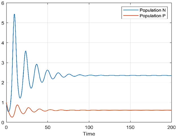
Figure 2. Time series of prey and predators when τ = 0.

The Figures 3, 4 represent the respectively the prey and the predator solution over time and space in domain [0, 100] × [0, π].

Figure 3

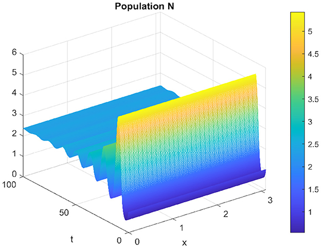
Figure 3. Spatiotemporal trajectory of prey when τ = 0.

Figure 4

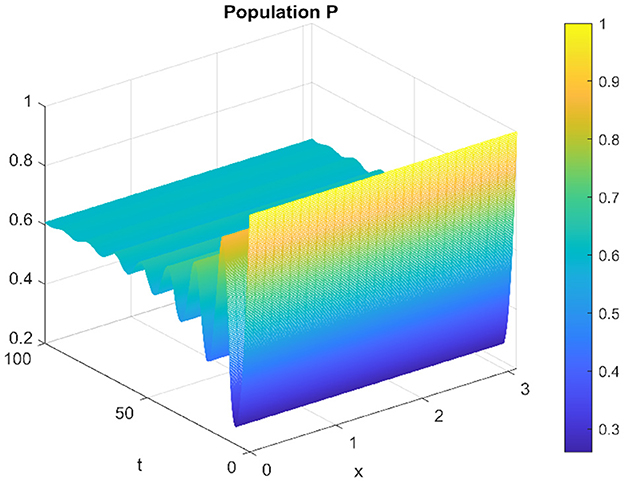
Figure 4. Spatiotemporal trajectory of predators when τ = 0.

For τ = 2.3 ∈ [0, τ^*], the system maintains its stability, which translates in Figures 5, 6.

Figure 5

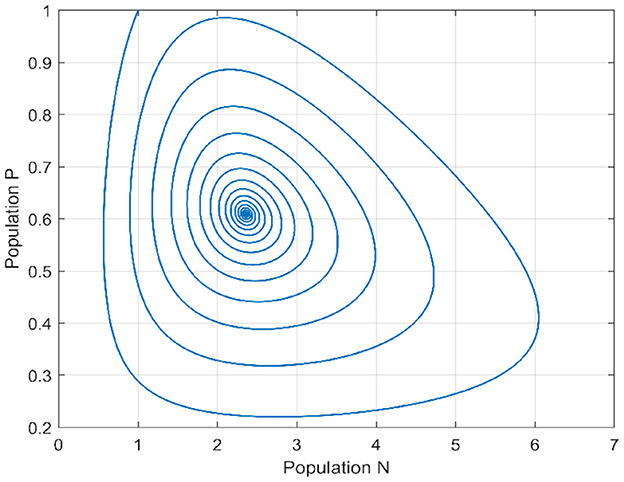
Figure 5. Phase portrait when τ = 2.3.

Figure 6

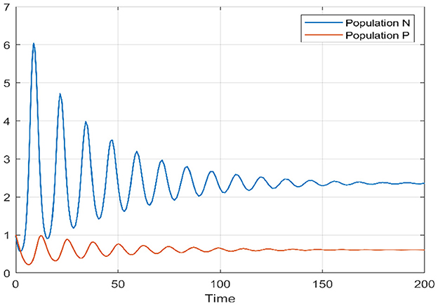
Figure 6. Time series of prey and predators when τ = 2.3.

Similarly, for the spatiotemporal case, the prey and the predator populations converge to the equilibrium point, as shown in Figures 7, 8.

Figure 7

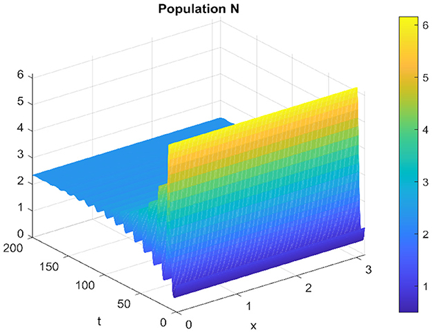
Figure 7. Spatiotemporal trajectory of prey when τ = 2.3.

Figure 8

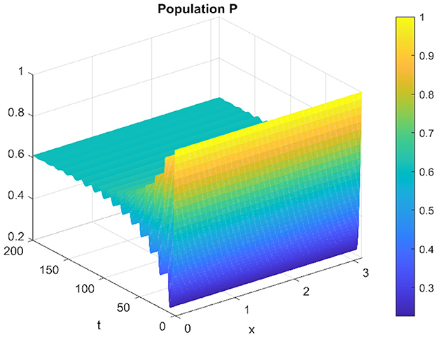
Figure 8. Spatiotemporal trajectory of predators when τ = 2.3.

For τ = 3.5, that is to say outside the stability interval associated with the model, we notice that the Equation 1 experiences a Hopf bifurcation, it loses its stability with the appearance of periodic solutions (see Figures 9, 10).

Figure 9

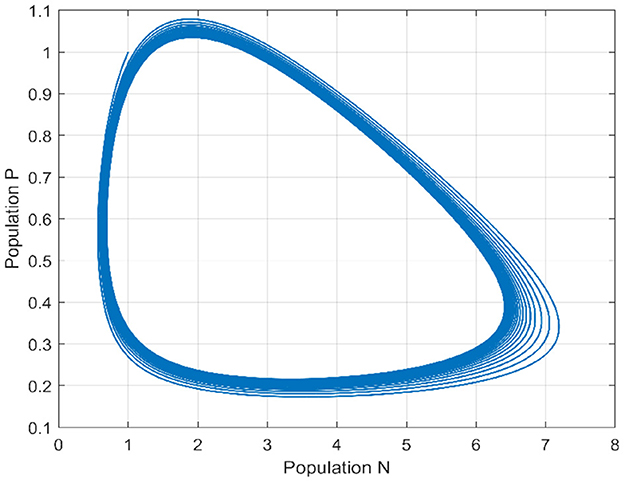
Figure 9. Phase portrait of Equation 2 when τ = 3.5.

Figure 10

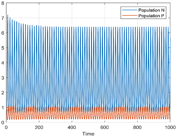
Figure 10. Time series of prey and predators when τ = 3.5.

Of the same for the spatiotemporal solution, which oscillates around the equilibrium point without converging. which is clear in the Figures 11, 12.

Figure 11

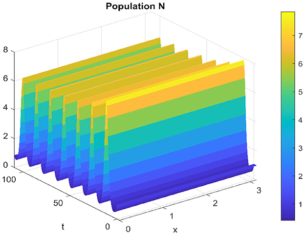
Figure 11. Spatiotemporal trajectory of prey when τ = 3.5.

Figure 12

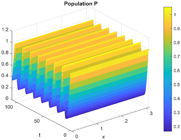
Figure 12. Spatiotemporal trajectory of predators when τ = 3.5.

In concluding this section, we present Figures 13, 14, showcasing the bifurcation diagrams associated with the delay for the prey and predators, respectively. These diagrams are constructed based on the minimum and maximum amplitudes of N (prey) and P (predators). The color differentiation within the diagrams signifies the nature of stability within the model: areas marked in blue delineate the stability interval, indicating regions where the model remains stable. A red star located at τ^* = 3.217 designates the bifurcation point, signifying a critical value where a qualitative change in the system's behavior occurs due to variations in delay. The green curve represents the interval of instability, indicating regions where the model exhibits instability. These bifurcation diagrams serve as visual representations, effectively capturing the complex dynamics associated with changes in delay. They provide an intuitive understanding of how the stability properties evolve concerning variations in delay, offering crucial insights into the system's behavior and transitions between stability and instability.

Figure 13

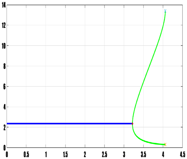
Figure 13. Bifurcation diagram of prey population.

Figure 14

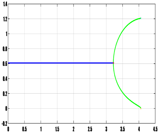
Figure 14. Bifurcation diagram of predator population.

5.2 Impact of diffusion coefficient

In the subsequent segment, our focus shifts toward understanding how alterations in the diffusion coefficient d₂ influence the dynamics of these populations. Employing identical parameters listed in the table and initiating the system from the point (2.358+0.001 × sin(πx), 0.609+0.001 × sin(πx)), we set τ = 0 and d₂ = 0.1. This deliberate selection adheres to verifying the Routh–Hurwitz condition, crucial for assessing the system's stability. Figures 15, 16 visually represent the outcomes of this analysis, demonstrating the model's stability under these specific conditions. These figures, presenting the phase portraits and solution trajectories over time for both prey and predators, reveal the system's behavior when subjected to variations in the diffusion coefficient d₂. The stability observed in these diagrams indicates the model's robustness and predictable dynamics under these prescribed parameters, allowing us to draw conclusions about the impact of d₂ on the overall system behavior.

Figure 15

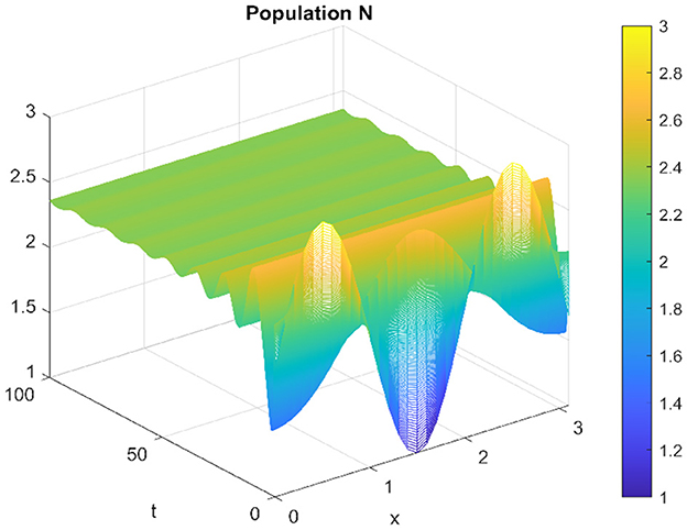
Figure 15. Spatiotemporal trajectory of prey when τ = 0 and d₂ = 0.1.

Figure 16

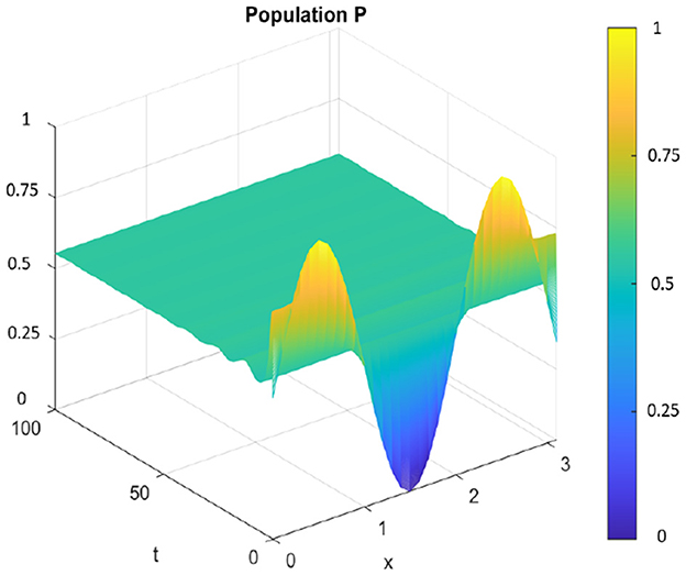
Figure 16. Spatiotemporal trajectory of predators when τ = 0 and d₂ = 0.1.

When altering the diffusion coefficient to d₂ = 0.01, while maintaining consistency in the values of other parameters, the positive equilibrium E^* remains stable for the ordinary differential equation (ODE) system. This means that the system exhibits stability and remains in an equilibrium state under these adjusted conditions. However, as per Theorem 11, the hypothesis H₂ of the theorem is validated, indicating a Turing instability in the spatiotemporal domain. This instability arises because the system attains a stable, nonconstant steady-state solution, causing the previously stable positive equilibrium E^* to become unstable. This transformation in stability properties is depicted in Figures 17, 18. The consequence of this instability is visually evident in the diagrams, where uneven spatial dispersion of populations is observed. This uneven distribution implies that the populations no longer maintain a homogeneous spread across space; instead, localized patterns emerge, indicative of spatial segregation or clustering within the ecosystem. This phenomenon showcases the intricate relationship between diffusion coefficients, stability properties, and spatial distribution, highlighting the system's propensity for spatially varied population distributions when subjected to specific parameter alterations.

Figure 17

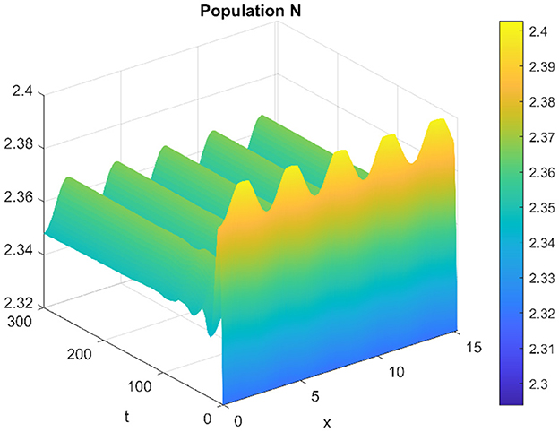
Figure 17. Spatiotemporal trajectory of prey when τ = 0 and d₂ = 0.01.

Figure 18

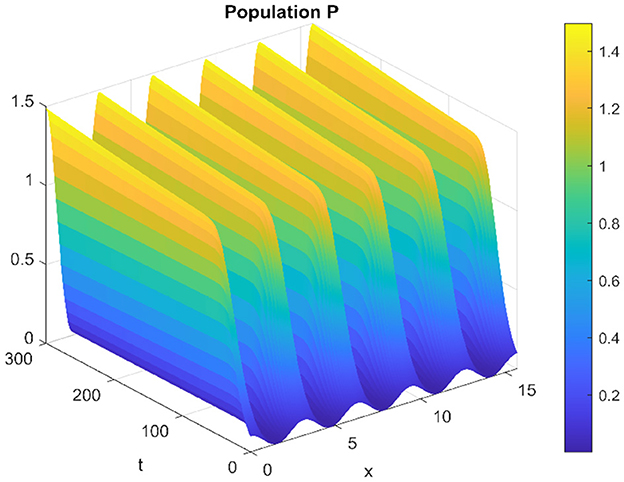
Figure 18. Spatiotemporal trajectory of predators when τ = 0 and d₂ = 0.01.

When τ = 3.22 and d₂ = 0.001, the system exhibits instability, fostering the existence of periodic inhomogeneous solutions. Under these conditions, a remarkable phenomenon emerges: the prey and predators coexist through spatially inhomogeneous oscillations. Notably, their densities manifest in opposing spatial distributions, a characteristic vividly visible in Figures 19, 20. These figures distinctly illustrate the spatial patterns where the densities of prey and predators display contrasting distributions within the ecosystem, signifying a spatial separation or differentiation that sustains their coexistence.

Figure 19

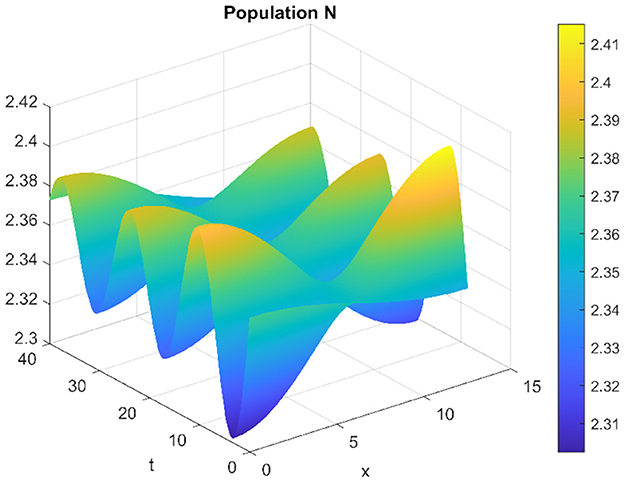
Figure 19. Spatiotemporal trajectory of prey when τ = 3.22 and d₂ = 0.001.

Figure 20

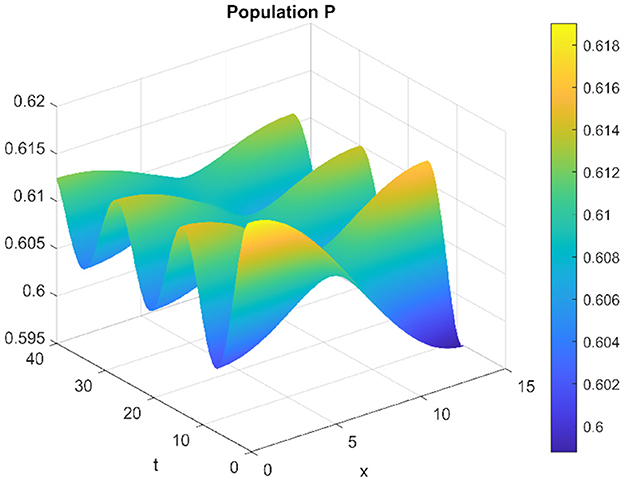
Figure 20. Spatiotemporal trajectory of predators when τ = 3.22 and d₂ = 0.001.

6 Discussion

The analysis of the delayed spatiotemporal predator-prey system provides valuable insights into the complex dynamics governing the interactions between predators and prey, incorporating various biological phenomena such as the Allee effect, fear effects on prey, cooperative hunting, the impact of toxicity, and differential fishing pressures on both species. Through this study, we have gained a better understanding of how these factors influence population dynamics by examining the stability and bifurcations of the system within both temporal and spatiotemporal frameworks.

In the temporal case, where diffusion coefficients are set to d₁ = d₂ = 0.1, we show that the positivity of the parameters α₀ and β₀ ensures the local asymptotic stability of the internal equilibrium point, as demonstrated by the model without delay. By analyzing the eigenvalue structure and verifying the Routh–Hurwitz conditions, we confirm that the equilibrium is stable for small perturbations, provided the delay remains within a specific stability interval [0, 3.217], as indicated by Theorems 4 and 11. The bifurcation diagrams (Figures 13, 14) offer a visual representation of the system's dynamics, highlighting the critical bifurcation point at τ^* = 3.217, beyond which a Hopf bifurcation leads to periodic oscillations in the populations.

In the spatiotemporal case, we observe that diffusion plays a significant role in the spatial distribution of predator and prey populations. When the system operates within the stability interval, the populations converge to the equilibrium point. However, as the delay exceeds this interval, the system undergoes periodic oscillations, and spatially inhomogeneous patterns emerge. These oscillations reflect the system's inability to maintain equilibrium, resulting in non-converging, oscillatory population densities. The behavior of the system also depends on the diffusion coefficient d₂, as variations in this parameter influence the stability of the system and the emergence of spatial patterns. When d₂ is reduced to 0.01, the positive equilibrium remains stable within the ODE system, but in the spatiotemporal case, this reduction induces a Turing instability, leading to the formation of spatial patterns. This instability arises from the heterogeneity induced by diffusion, even though the temporal dynamics remain stable, illustrating how diffusion can destabilize spatial equilibrium.

Reducing d₂ to 0.001 and increasing the delay to τ = 3.22 exacerbates the instability of the system, supporting spatially inhomogeneous periodic solutions. These oscillations lead to spatial segregation between predator and prey, with high prey densities corresponding to low predator densities, and vice versa. This spatial separation is characteristic of ecological systems where environmental factors, habitat fragmentation, or localized resource availability cause spatial differentiation between prey and predator populations.

These results highlight the resilience of the predator-prey system in maintaining coexistence, even under complex conditions of spatial segregation. It demonstrates the model's ability to predict complex ecological behaviors, such as patchiness and species clustering in shared environments, where diffusion-induced instability and temporal delays govern population dynamics. Our findings align with recent studies on diffusive predator-prey systems incorporating time delays and spatial heterogeneity [4, 34, 37], yet they also introduce new perspectives on the role of fishing pressures and toxicity. For example, in Yang et al. [4], nonlocal competition was shown to induce spatially inhomogeneous bifurcating periodic solutions. Similarly, our model reveals that reducing the diffusion coefficient d₂ triggers Turing instabilities, leading to spatial pattern formation, suggesting that diffusion-driven instabilities can arise in different ecological scenarios, whether due to competition mechanisms or differential movement rates.

In Song et al. [34], the impact of time delays in a system with a generalist predator was studied, showing that delays induce oscillatory behavior. Our results corroborate this, particularly with the Hopf bifurcation observed at τ = 3.217, marking the transition from stability to periodic oscillations. However, our study extends this analysis by incorporating the combined effects of spatial diffusion and delay, demonstrating that these factors together drive more complex spatial dynamics, such as predator-prey segregation. Moreover, in Yang et al. [37], the authors examined how habitat complexity influences predator-prey interactions. While their model highlights the role of environmental structure, our approach distinguishes itself by explicitly considering how spatial heterogeneity, coupled with diffusion and delay, can generate inhomogeneous patterns without assuming pre-existing habitat constraints. This distinction is crucial for understanding how spatial structures emerge from intrinsic system dynamics, rather than being shaped by external environmental factors. This perspective is particularly relevant for understanding how real-world ecosystems, where predator and prey distributions are influenced by both internal dynamics and external pressures, function and evolve.

The results obtained from this delayed spatiotemporal predator-prey model emphasize the importance of spatial diffusion and time delays in generating complex predator-prey dynamics. These factors play a key role in determining population persistence, stability, and spatial organization, providing a more comprehensive framework for analyzing predator-prey interactions in both managed and natural ecosystems. By considering the interplay between biological and environmental factors, including toxicity and fishing pressures, we gain a deeper understanding of the ecological behaviors that emerge from complex predator-prey systems.

7 Conclusion

This study provides a detailed analysis of a delayed spatiotemporal predator-prey system, integrating various biological and environmental factors, such as the Allee effect, fear effects on prey, cooperative hunting, toxicity, and fishing pressures. Our results reveal that time delays significantly impact the system's stability, leading to periodic oscillations when delays cross a critical threshold. This finding aligns with previous studies, such as those Chakrabortyet al. [45], which observed similar oscillatory behavior in predator-prey models with delays. However, our model extends these findings by incorporating spatial diffusion, which, when altered, induces Turing instabilities and the formation of spatial patterns. While Shukla et al. [20] demonstrated how diffusion can create spatially inhomogeneous patterns in algal blooms, our work applies this concept to predator-prey interactions, showing how diffusion, combined with delays, leads to spatial segregation between predator and prey populations. Furthermore, our study introduces the impact of external pressures such as fishing and toxicity, which are absent in previous models like those of Maity et al. [19], who focused on eco-epidemic dynamics. By incorporating these factors, we provide a more comprehensive understanding of how human interventions destabilize predator-prey systems, a nuance not captured in earlier works. Lastly, our study confirms the spatial patchiness observed in ecological systems, a feature explored in Maity et al. [19], but extends it by showing that such patterns can emerge purely from the internal dynamics of the system, without relying on pre-existing habitat structures, unlike studies that emphasized habitat complexity. Overall, this work builds upon and extends previous research by integrating both internal and external factors, offering a more holistic understanding of predator-prey dynamics in complex ecosystems. In future research, this model could be extended by incorporating stochastic environmental effects and age-structured populations, which would allow for a more realistic representation of ecological uncertainty. Additionally, validating the model using empirical data from real ecosystems would enhance its practical applicability and support the development of more effective management strategies for predator-prey systems under human pressure.

Data availability statement

The original contributions presented in the study are included in the article/supplementary material, further inquiries can be directed to the corresponding author.

Author contributions

MH: Writing – original draft. NB: Writing – original draft. YE: Supervision, Writing – original draft. NA: Supervision, Writing – original draft.

Funding

The author(s) declare that no financial support was received for the research and/or publication of this article.

Conflict of interest

The authors declare that the research was conducted in the absence of any commercial or financial relationships that could be construed as a potential conflict of interest.

Generative AI statement

The author(s) declare that no Gen AI was used in the creation of this manuscript.

Publisher's note

All claims expressed in this article are solely those of the authors and do not necessarily represent those of their affiliated organizations, or those of the publisher, the editors and the reviewers. Any product that may be evaluated in this article, or claim that may be made by its manufacturer, is not guaranteed or endorsed by the publisher.

References

1. Song Y, Shi Q. Stability and bifurcation analysis in a diffusive predator-prey model with delay and spatial average. Math Methods Appl Sci. (2022) 46:5561–84. doi: 10.1002/mma.8853

Crossref Full Text | Google Scholar

2. Xiang C, Huang J, Wang H. Bifurcations in Holling-Tanner model with generalist predator and prey refuge. J Differ Equ. (2023) 343:495–529. doi: 10.1016/j.jde.2022.10.018

Crossref Full Text | Google Scholar

3. Vatsala AS, Pageni G. Series solution method for solving sequential Caputo fractional differential equations. AppliedMath. (2023) 3:730–40. doi: 10.3390/appliedmath3040039

Crossref Full Text | Google Scholar

4. Yang R, Nie C, Jin D. Spatiotemporal dynamics induced by nonlocal competition in a diffusive predator-prey system with habitat complexity. Nonlinear Dyn. (2022) 110:879–900. doi: 10.1007/s11071-022-07625-x

Crossref Full Text | Google Scholar

5. Yang R, Wang F, Jin D. Spatially inhomogeneous bifurcating periodic solutions induced by nonlocal competition in a predator-prey system with additional food. Math Methods Appl Sci. (2022) 45:9967–78. doi: 10.1002/mma.8349

Crossref Full Text | Google Scholar

6. Hafdane M, Boutayeb H, Agmour I, El Foutayeni Y, Achtaich N. The role of cleaner fish in a predator-prey model: dynamics and optimal harvesting. Commun Math Biol Neurosci. (2023) 2023:92.

Google Scholar

7. Bhattacharyya J, Pal S. Stage-structured cannibalism with delay in maturation and harvesting of an adult predator. J Biol Phys. (2013) 39:37–65. doi: 10.1007/s10867-012-9284-6

PubMed Abstract | Crossref Full Text | Google Scholar

8. Bhattacharyya J, Pal S. Hysteresis in coral reefs under macroalgal toxicity and overfishing. J Biol Phys. (2015) 41:151–72. doi: 10.1007/s10867-014-9371-y

PubMed Abstract | Crossref Full Text | Google Scholar

9. Cresswell W. Predation in bird populations. J Ornithol. (2011) 152:251–63. doi: 10.1007/s10336-010-0638-1

Crossref Full Text | Google Scholar

10. Xie B. Impact of the fear and Allee effect on a Holling type II prey-predator model. Adv Differ Equ. (2021) 2021:1–15. doi: 10.1186/s13662-021-03592-6

Crossref Full Text | Google Scholar

11. Hale JK. Theory of Functional Differential Equations. New York, NY: Springer (1977). doi: 10.1007/978-1-4612-9892-2

Crossref Full Text | Google Scholar

12. Hafdane M, Collera JA, Agmour I, El Foutayeni Y. Hopf bifurcation for delayed prey-predator system with Allee effect. Commun Math Biol Neurosci. (2023) 2023:36. Available online at: https://scik.org/index.php/cmbn/article/view/7921

Google Scholar

13. Baba N, Idmbarek A, Bendahou FE, et al. Navigating the Allee effect: unraveling the influence on marine ecosystems. J Coast Conserv. (2023) 27:65. doi: 10.1007/s11852-023-00989-1

Crossref Full Text | Google Scholar

14. Baba N, Agmour I, El Foutayeni Y, Achtaich N. Toxicity impacts on bioeconomic models of phytoplankton and zooplankton interactions. Ocean Dyn. (2023). 74:53–66. doi: 10.1007/s10236-023-01588-2

Crossref Full Text | Google Scholar

15. Chakraborty S, Tiwari PK, Sasmal SK, Biswas S, Bhattacharya S, Chattopadhyay J, et al. Interactive effects of prey refuge and additional food for predator in a diffusive predator-prey system. Appl Math Model. (2017) 47:128–40. doi: 10.1016/j.apm.2017.03.028

Crossref Full Text | Google Scholar

16. Allee WC. Animal aggregations. In: A Study in General Sociology. Chicago, IL: University of Chicago Press (1931). doi: 10.5962/bhl.title.7313

PubMed Abstract | Crossref Full Text | Google Scholar

17. Liu J. Qualitative analysis of a diffusive predator-prey model with Allee and fear effects. Int J Biomath. (2021) 14:2150037. doi: 10.1142/S1793524521500376

Crossref Full Text | Google Scholar

18. Lai L, Zhu Z, Chen F. Stability and bifurcation in a predator-prey model with the additive Allee effect and the fear effect. Mathematics. (2020) 8:1280. doi: 10.3390/math8081280

Crossref Full Text | Google Scholar

19. Maity SS, Tiwari PK, Shuai Z, Pal S. Role of space in an eco-epidemic predator-prey system with the effect of fear and selective predation. J Biol Syst. (2023) 31:883–920. doi: 10.1142/S0218339023500316

Crossref Full Text | Google Scholar

20. Shukla JB, Misra AK, Sundar S. Effect of cross-diffusion on the patterns of algal bloom in a lake: a nonlinear analysis. Nonlinear Stud. (2014) 21.

Google Scholar

21. Chakraborty K, Das S, Kar TK. Optimal control of effort of a stage-structured prey-predator fishery model with harvesting. Nonlinear Anal Real World Appl. (2011) 12:3452–67. doi: 10.1016/j.nonrwa.2011.06.007

Crossref Full Text | Google Scholar

22. Ang TK, Safuan HM. Dynamical behaviors and optimal harvesting of an intraguild prey-predator fishery model with Michaelis-Menten type predator harvesting. Biosystems. (2021) 202:104357. doi: 10.1016/j.biosystems.2021.104357

PubMed Abstract | Crossref Full Text | Google Scholar

23. Hu P, Cao HJ. Stability and bifurcation analysis in a predator-prey system with Michaelis-Menten type predator harvesting. Nonlinear Anal Real World Appl. (2017) 33:58–82. doi: 10.1016/j.nonrwa.2016.05.010

Crossref Full Text | Google Scholar

24. Guo HJ, Chen LS. The effects of impulsive harvest on a predator-prey system with distributed time delay. Commun Nonlinear Sci Numer Simul. (2009) 14:2301–9. doi: 10.1016/j.cnsns.2008.05.010

Crossref Full Text | Google Scholar

25. Dou J, Li S. Optimal impulsive harvesting policies for single-species populations. Appl Math Comput. (2017) 292:145–55. doi: 10.1016/j.amc.2016.07.027

Crossref Full Text | Google Scholar

26. Li W, Ji J, Huang L. Global dynamic behavior of a predator-prey model under ratio-dependent state impulsive control. Appl Math Model. (2020) 77:1842–59. doi: 10.1016/j.apm.2019.09.033

Crossref Full Text | Google Scholar

27. Tang SY, Pang WH, Cheke RA, Wu JH. Global dynamics of a state-dependent feedback control system. Adv Diff Equ. (2015) 2015:322. doi: 10.1186/s13662-015-0661-x

Crossref Full Text | Google Scholar

28. Zhang T, Ma W, Meng X, Zhang T. Periodic solution of a prey-predator model with nonlinear state feedback control. Appl Math Comput. (2015) 266:95–107. doi: 10.1016/j.amc.2015.05.016

Crossref Full Text | Google Scholar

29. Huang MZ, Liu SZ, Song XY, Chen LS. Dynamics of unilateral and bilateral control systems with state feedback for renewable resource management. Complexity. (2020) 2020:9453941. doi: 10.1155/2020/9453941

Crossref Full Text | Google Scholar

30. Hocking LM. Optimal Control: An Introduction to the Theory with Applications. Oxford: Oxford University Press (1991). doi: 10.1093/oso/9780198596752.001.0001

Crossref Full Text | Google Scholar

31. Xiao ZLi Z, et al. Stability analysis of a mutual interference predator-prey model with the fear effect. J Appl Sci Eng. (2019) 22:205–11.

Google Scholar

32. Sasmal SK, Takeuchi Y. Dynamics of a predator-prey system with fear and group defense. J Math Anal Appl. (2020) 481:123471. doi: 10.1016/j.jmaa.2019.123471

Crossref Full Text | Google Scholar

33. Bendahou FE, Baba N, El Foutayeni Y, Achtaich N. Impact of pollution on sardine, sardinella, and mackerel fishery: a bioeconomic approach. Commun Math Biol Neurosci. (2023) 2023:55.

Google Scholar

34. Song Y, Peng Y, Zhang T. The spatially inhomogeneous Hopf bifurcation induced by memory delay in a memory-based diffusion system. J Differ Equ. (2021) 300:597–624. doi: 10.1016/j.jde.2021.08.010

PubMed Abstract | Crossref Full Text | Google Scholar

35. Akhmet MU, Beklioglu M, Ergenc T, Tkachenko VI. An impulsive ratio-dependent predator-prey system with diffusion. Nonlinear Anal Real World Appl. (2006) 7:1255–67. doi: 10.1016/j.nonrwa.2005.11.007

PubMed Abstract | Crossref Full Text | Google Scholar

36. Liu Y, Wei J. Double Hopf bifurcation of a diffusive predator-prey system with strong Allee effect and two delays. Nonlinear Anal Model Control. (2021) 26:72–92. doi: 10.15388/namc.2021.26.20561

Crossref Full Text | Google Scholar

37. Yang R, Jin D, Wang W. A diffusive predator-prey model with generalist predator and time delay. AIMS Math. (2022) 7:4574–91. doi: 10.3934/math.2022255

Crossref Full Text | Google Scholar

38. Alikakos ND. An application of the invariance principle to reaction-diffusion equations. J Differ Equ. (1979) 33:201–25. doi: 10.1016/0022-0396(79)90088-3

Crossref Full Text | Google Scholar

39. Ni WM, Tang M. Turing patterns in the Lengyel-Epstein system for the CIMA reaction. Trans Am Math Soc. (2005) 357:3953–69. doi: 10.1090/S0002-9947-05-04010-9

PubMed Abstract | Crossref Full Text | Google Scholar

40. Banerjee M, Takeuchi Y. Maturation delay for the predators can enhance stable coexistence for a class of prey-predator models. J Theor Biol. (2017) 412:154–71. doi: 10.1016/j.jtbi.2016.10.016

PubMed Abstract | Crossref Full Text | Google Scholar

41. Meng X, Jiao J, Chen L. The dynamics of an age-structured predator-prey model with disturbing pulse and time delays. Nonlinear Anal Real World Appl. (2008) 9:547–61. doi: 10.1016/j.nonrwa.2006.12.001

Crossref Full Text | Google Scholar

42. Hafdane M, Agmour I, El Foutayeni Y. Study of Hopf bifurcation of delayed tritrophic system: dinoflagellates, mussels, and crabs. Math Model Comput. (2023) 10:66–79. doi: 10.23939/mmc2023.01.066

Crossref Full Text | Google Scholar

43. Joy RA, Hawlader MS, Rahman MS, Hossain MR, Shamim SI, Mahmud H, et al. Improving quality, productivity, and cost aspects of a sewing line of apparel industry using TQM approach. Math Probl Eng. (2024) 2024:6697213. doi: 10.1155/2024/6697213

Crossref Full Text | Google Scholar

44. La Torre D, Kunze H, Ruiz-Galan M, Malik T, Marsiglio S. Optimal control: theory and application to science, engineering, and social sciences. Abstr Appl Anal. (2015) 2015:890527. doi: 10.1155/2015/890527

Crossref Full Text | Google Scholar

45. Chakraborty S, Tiwari PK, Misra AK, Chattopadhyay J. Spatial dynamics of a nutrient–phytoplankton system with toxic effect on phytoplankton. Math Biosci. (2015) 264:94–100. doi: 10.1016/j.mbs.2015.03.010

PubMed Abstract | Crossref Full Text | Google Scholar

46. Stephens PA, Sutherland WJ. Consequences of the Allee effect for behavior, ecology, and conservation. Trends Ecol Evol. (1999) 14:401–5. doi: 10.1016/S0169-5347(99)01684-5

PubMed Abstract | Crossref Full Text | Google Scholar

47. Berec L, Angulo E, Courchamp F. Multiple Allee effects and population management. Trends Ecol Evol. (2007) 22:185–91. doi: 10.1016/j.tree.2006.12.002

PubMed Abstract | Crossref Full Text | Google Scholar

48. Cantrell RS, Cosner C, Hutson V. Permanence in ecological systems with spatial heterogeneity. Proc R Soc Edinb A Math. (1993) 123:533–59. doi: 10.1017/S0308210500025877

Crossref Full Text | Google Scholar

49. Zanette LY, White AF, Allen MC, Clinchy M. Perceived predation risk reduces the number of offspring songbirds produce per year. Science. (2011) 334:1398–401. doi: 10.1126/science.1210908

PubMed Abstract | Crossref Full Text | Google Scholar

50. Courchamp F, Clutton-Brock T, Grenfell B. Inverse density dependence and the Allee effect. Trends Ecol Evol. (1999) 14:405–10. doi: 10.1016/S0169-5347(99)01683-3

PubMed Abstract | Crossref Full Text | Google Scholar