Plug-and-play low-rank tensor completion and reconstruction algorithms with improved applicability of tensor decompositions

In this paper, we propose a new unified optimization algorithm for general tensor completion and reconstruction problems, which is formulated as an inverse problem for low-rank tensors in general linear observation models. The proposed algorithm supports at least three basic loss functions (ℓ₂ loss, ℓ₁ loss, and generalized KL divergence) and various TD models (CP, Tucker, TT, TR decompositions, non-negative matrix/tensor factorizations, and other constrained TD models). We derive the optimization algorithm based on a hierarchical combination of the alternating direction method of multipliers (ADMM) and majorization-minimization (MM). We show that the proposed algorithm can solve a wide range of applications and can be easily extended to any established TD model in a plug-and-play manner.

1 Introduction

Tensor decompositions (TDs) are beginning to be used in various fields of applications such as image recovery [1], blind source separation [2], traffic data analysis [3], wireless communications [4], and quantum state tomography [5–7]. Tensor decompositions are mathematical models that are used directly to exploit the low-rank structure of tensors [8–10]. In addition, other various optional structures such as non-negativity [11–13], sparsity [14–17], smoothness [18–21], and manifold constraints [22–24] can be incorporated into factor matrices or core tensors in tensor decompositions. Such flexible modeling in tensor decompositions makes it popular for wide applications. In applications of tensor decompositions, various data analysis tasks can be addressed by designing optimization problems based on the assumptions of low-rank and other additional data structures and optimizing parameters to maximize the consistency (likelihood) with the observed data.

The challenges of applying tensor decomposition to each data analysis task are 2-fold. First, it is necessary to appropriately design TD models and optimization problems with constraints according to the objective of each data analysis task and the observation model of measurement data, which requires deep domain-specific insight and experience. The second challenge is to derive and implement an efficient optimization algorithm for the designed specific tensor decomposition problem, which requires high-level computer science skills such as applied linear algebra, numerical computation, mathematical optimization, and programming languages. Overcoming these two challenges is not easy, as it is rare to find someone who is both an expert in a specific domain and well-versed in computer science. Constructing a project team that includes experts in the specific domain and computer science for this purpose can be useful, but costs remain high. The first challenge is closely related to research in the target domain and will be difficult to solve fundamentally. However, the second challenge can be solved by technological advances. Here, we will move on to the discussion of solving the second challenge.

In conventional research, a new tensor modeling method is proposed to solve a specific task, the corresponding optimization algorithm is derived, implemented, and experimented on, and the whole is published as a single paper. This research approach is common and robust, but it is very costly because a custom optimization algorithm must be derived and implemented for each subdivided problem. For example, the problem of recovering tensor data that includes missing values is known as the tensor completion problem [25–29]. Now, if we consider a model in which the true tensor is low Tucker/CP rank, the core tensor or factor matrices are non-negative, and the observations contain Gaussian noise, the optimization problem can be formulated as a non-negative Tucker/CP decomposition with missing values based on ℓ₂ loss minimization. It is possible to derive and implement specific optimization algorithms with some expertise [30, 31]. However, in some applications, one often wants to change the assumed noise distribution, try different TD models, or add constraints to the factor matrices [32–37]. It would be possible to derive and implement a specific optimization algorithm each time such a model change is made, but this would be very costly.

One approach to solving the above problems is to develop a universal optimization algorithm that can solve a variety of data analysis problems based on tensor decomposition. Having a single universal solver frees most users from the requirements of derivation and implementation of individual algorithms, allowing them to focus on designing the models. This environment will encourage users to iterate through trial-and-error modeling and accelerate applications of tensor decomposition. The technical challenge in developing a universal optimization algorithm is how to formulate the problem and how to design the structure of the algorithm. A universal optimization algorithm needs to efficiently connect various TD models to various reconstruction problems, but finding the method is not trivial.

In this paper, as a major step toward this goal, we propose a unified algorithm for obtaining any tensor decomposition under various noisy linear observation models. The proposed algorithm supports three basic loss functions (ℓ₂ loss, ℓ₁ loss, and generalized KL divergence) and various low-rank TD models. Since our formulation is considered as a general linear observation model, the proposed algorithm can address a variety of problems such as noise removal, tensor completion, deconvolution, super-resolution, compressed sensing, and medical imaging [1].

We derive the optimization algorithm based on the hierarchical combination of the alternating direction method of multipliers (ADMM) [38], majorization-minimization (MM) [39, 40] algorithm and least-squares (LS) based tensor decomposition. The most distinctive feature of our approach is that it uses LS-based tensor decompositions as plug-and-play modules (denoisers). LS-based algorithms have been well established for various types of TD such as canonical polyadic decomposition (CPD) [41–43], Tucker decomposition (TKD) [44–48], tensor-train decomposition (TTD) [49, 50], tensor-ring decomposition (TRD) [51], and non-negative matrix/tensor factorizations (NMF/NTF) [11, 52, 53]. Next, we derive an MM algorithm for solving the tensor decomposition problem in a linear observation model based on ℓ₂ loss (Gaussian noise). Since various TD algorithms can be adopted as modules, we can support various TD models at this point. Finally, we derive an ADMM to minimize the ℓ₁ loss and the generalized KL divergence for observations under Laplace and Poisson noises. As a result, an overall ADMM algorithm calls MM in the loop, and the MM calls TD algorithms for the update rule.

It should be noted that the structure of the proposed algorithm can incorporate different TD models in a plug-and-play (PnP) manner. This is inspired by work that applies arbitrary denoisers in a plug-and-play manner in image reconstruction such as PnP-ADMM [54]. LS-based TD can be viewed as a denoising that the low-rank tensor reconstruction from noisy tensor. In our study, we only assume the existence of LS-based TD algorithms and therefore also include undiscovered TD models that will be proposed in the future. In addition, the proposed framework can be easily extended for penalized matrix/tensor decompositions. Many sophisticated TD models can be applied as prior to linear inverse problems. For example, our method allows some sophisticated decomposition models proposed for tensor completion to be easily extended to other tasks such as robust tensor decomposition, deconvolution, compressive sensing, and computed tomography.

1.1 Notations

A vector, a matrix, and a tensor are indicated by a bold lowercase letter, a ∈ ℝ^I, a bold uppercase letter, B ∈ ℝ^{I × J}, and a bold calligraphic letter, $C$ ∈ ℝ^{J₁ × J₂ × ⋯ × J_N}, respectively. An Nth-order tensor, $X$ ∈ ℝ^{I₁ × I₂ × ⋯ × I_N}, can be transformed into a vector, which is denoted by using the same character, $\mathbf{\text{x}}=\mathrm{\text{vec}}(X)\in ℝ{\prod }_{n=1}^N{I}_n$. An (i₁, i₂, ..., i_N)-element of $X$ is denoted by x_{i1, i2, ..., iN} or [$X$]_{i1, i2, ..., iN}. The operators ⊡ represent the Hadamard product. ·^† represents the Moore-Penrose pseudoinverse. sign($X$) ∈ ℝ^{I₁ × I₂ × ⋯ × I_N} and abs($X$) ∈ ℝ^{I₁ × I₂ × ⋯ × I_N} are, respectively, operations that return the sign and absolute value for each entry of $X$ ∈ ℝ^{I₁ × I₂ × ⋯ × I_N}.

2 Review of existing tensor completion and reconstruction methods from a perspective of plug-and-play algorithms

2.1 LS-based tensor decomposition

Tensor decomposition (TD) is a mathematical model to represent a tensor as a product of tensors/matrices. There are many TD models such as canonical polyadic decomposition (CPD) [41–43, 55], Tucker decomposition (TKD) [44–46], tensor-train decomposition (TTD) [49, 50], tensor-ring decomposition (TRD) [51], block-term decomposition [56–58], coupled tensor decomposition [59–61], hierarchical Tucker decomposition [62], tensor wheel decomposition [63], fully connected tensor network [64], t-SVD [65], Hankel tensor decomposition [66–69], and convolutional tensor decomposition [21].

Figure 1 shows typical models of tensor decompositions in graphical notation [10]. In graphical notation, each node represents a core tensor and the edges connecting the nodes represent tensor products. As can be seen in the figure, all TD models are expressed by tensor products of core tensors.

Figure 1

Figure 1. Tensor decomposition models in graphical notation.

In this paper, we will write any TD model as

$\begin{array}{ll}X=\langle \langle G_1,G_2,...,G_L\rangle \rangle \in {ℝ}^{I_1\times I_2\times \cdots \times I_N}.& (1)\end{array}$

Note that Equation 1 is a somewhat abstract expression which only represents that the entire tensor $X$ is reconstructed by multiplying the L core tensors $G$₁, $G$₂, ..., $G$_L−1 and $G$_L. The least squares (LS) based tensor decomposition problem of a given tensor $V$ ∈ ℝ^{I₁ × I₂ × ⋯ × I_N} is given by

$\begin{array}{ll}(G_1^{*},G_2^{*},...,G_L^{*})=\underset{G_1,G_2,...,G_L}{\text{argmin}}\parallel V-\langle \langle G_1,G_2,...,G_L\rangle \rangle {\parallel }_F^2.& (2)\end{array}$

This squared error is a non-convex function with respect to overall optimization parameters ($G$₁, $G$₂, ..., $G$_L), but it is a convex quadratic function with respect to only one core tensor $G$_l for any l ∈ {1, 2, ..., L}. If we focus on optimizing a certain core tensor $G$_l and temporarily consider all other core tensors as constant variables and can be summarized as a single tensor, denoted as $G$_−l, then the sub-optimization problem is reduced to an LS-based matrix optimization problem:

$\begin{array}{l}\underset{G_l}{\text{argmin}}\parallel V-\langle \langle G_l,G_{-l}\rangle \rangle {\parallel }_F^2\\ =\underset{G_l}{\text{argmin}}\parallel {\text{mat}}_{l1}(V)-{\text{mat}}_{l2}(G_l){\text{mat}}_{l3}(G_{-l}){\parallel }_F^2,& (3)\end{array}$

where we used abstract notations 〈〈$G$_l, $G$_−l〉〉 = 〈〈$G$₁, $G$₂, ..., $G$_L〉〉, and mat_lm, m ∈ {1, 2, 3}, are the corresponding appropriate matricization operators for the certain l-th core tensor. Solving sub-optimization shown in Equation 3 has a closed-form solution and updating $G$_l by

$\begin{array}{ll}{G}_l\leftarrow {\text{mat}}_{l2}^{-1}\left({\text{mat}}_{l1}(V){\text{mat}}_{l3}{(G_{-l})}^{†}\right)& (4)\end{array}$

always reduces (non-increases) the squared error. In other words, putting θ = ($G$₁, $G$₂, ..., $G$_L) and $f(\theta )=\parallel V-\langle \langle G_1,G_2,...,G_L\rangle \rangle {\parallel }_F^2$, the following algorithm

$\begin{array}{ll}{\theta }_k\leftarrow (G_1,G_2,\mathrm{...},G_L);& (5)\end{array}$

$\begin{array}{ll}{G}_l\leftarrow {\text{mat}}_{l2}^{-1}\left({\text{mat}}_{l1}(V){\text{mat}}_{l3}{(G_{-l})}^{†}\right);& (6)\end{array}$

$\begin{array}{ll}{\theta }_{k+1}\leftarrow (G_1,G_2,\mathrm{...},G_L);& (7)\end{array}$

provides the result f(θ_k) ≥ f(θ_k+1) for any l ∈ {1, 2, ..., L}. Therefore, the LS-based tensor decomposition problem in Equation 2 can be solved by repeating the steps shown in Equation 6 for every l ∈ {1, 2, ..., L}, and this is called the alternating least squares (ALS) algorithm [42, 43, 47, 50, 51]. ALS is a workhorse algorithm in TDs because it has no hyper-parameter (e.g., step-size of gradient descent), and the objective function can be stably reduced (monotonically non-increasing).

2.1.1 Perspective on optimizing $X$ by ALS

Here, let us interpret that the ALS algorithm optimizes $X$ rather than ($G$₁, $G$₂, ..., $G$_L). This does not make any difference in the process. The LS-based low-rank tensor optimization problem can be formulated by

$\begin{array}{ll}{X}^{*}=\underset{X}{\text{argmin}}\parallel V-X{\parallel }_F^2+i_{{𝕊}_t}(X),& (8)\end{array}$

where 𝕊_t ⊂ ℝ^{I₁ × I₂ × ⋯ × I_N} is a set of low-rank tensors which have tensor decomposition 〈〈$G$₁, $G$₂, ..., $G$_L〉〉,

$\begin{array}{ll}{𝕊}_t:=\{\langle \langle G_1,G_2,...,G_L\rangle \rangle |G_1\in D_1,G_2\in D_2,...,G_L\in D_L\},& (9)\end{array}$

$D$_l is a domain of $G$_l and i_𝕊t($X$) is an indicator function

$\begin{array}{ll}{i}_{{𝕊}_t}(X)=\{\begin{array}{cc}0& X\in {𝕊}_t\\ \infty & \text{otherwise}\end{array}.& (10)\end{array}$

Since the objective functions in Equations 2, 8 are the same when $X$ = 〈〈$G$₁, $G$₂, ..., $G$_L〉〉, their minimizers also satisfy $X^{*}=\langle \langle G_1^{*},G_2^{*},...,G_L^{*}\rangle \rangle$ if $X$^* is unique. Note that the core tensors are generally non-unique (e.g., we have $\langle \langle G_1,G_2,...,G_L\rangle \rangle =\langle \langle c{G}_1,c^{-1}{G}_2,...,G_L\rangle \rangle$ for any c ≠ 0).

Remark 1. If $X$^* is unique, then the solutions to the problems shown in Equations 2, 8 satisfy $X^{*}=\langle \langle G_1^{*},G_2^{*},...,G_L^{*}\rangle \rangle$.

In practice, $X$^* may not be unique, but even then there will always be a pair of solutions such that $X^{*}=\langle \langle G_1^{*},G_2^{*},...,G_L^{*}\rangle \rangle$. Hence, the problem in Equation 8 can be solved by ALS. Updating the core tensors θ by ALS simultaneously implies updating $X$. Since the series θ₀ → θ₁ → ⋯ → θ_∞ results in $X$₀→$X$₁ → ⋯ → $X$_∞, we pay attention to the fact that the ALS produces a series of {$X$_k} here. In this paper, we denote the operation of updating $X$ by ALS as

$\begin{array}{ll}{X}_{k+1}={\mathcal{U}}_{V,{𝕊}_t}^{\text{ALS}}(X_k),& (11)\end{array}$

where ${\mathcal{U}}_{V,{𝕊}_t}^{\mathrm{\text{ALS}}}:{𝕊}_t\to {𝕊}_t$ can be considered as an interior point algorithm to a point closer to $V$:

$\begin{array}{ll}\parallel V-{\mathcal{U}}_{V,{𝕊}_t}^{\text{ALS}}(X){\parallel }_F\le \parallel V-X{\parallel }_F& (12)\end{array}$

for any $X$ ∈ 𝕊_t. Although it is omitted in Equation 11, it is essential for implementation that the input and output of ${\mathcal{U}}_{V,{𝕊}_t}^{\mathrm{\text{ALS}}}$ include not only $X$ but also θ. We suppose that an operation ${\mathcal{U}}_{V,{𝕊}_t}^{\mathrm{\text{ALS}}}$ outputs a reconstructed tensor resulting from updating at least once for all core tensors. The approximate solution to the problem shown in Equation 8 can be found by repeating the ALS update sufficiently as

$\begin{array}{ll}{X}^{*}\approx {\text{Proj}}_{{𝕊}_t}^{\text{ALS}}(V,X_0):={\mathcal{U}}_{V,{𝕊}_t}^{\text{ALS}}°\cdots °{\mathcal{U}}_{V,{𝕊}_t}^{\text{ALS}}(X_0),& (13)\end{array}$

where $X$₀ ∈ 𝕊_t is some initialization of $X$. Here, the entire ALS is represented as ${\mathrm{\text{Proj}}}_{{𝕊}_t}^{\mathrm{\text{ALS}}}(V,X_0)$. This is because Equation 8 is a problem in finding the closest point in 𝕊_t from a point $V$, and it is just a projection of $V$ onto 𝕊_t. Note that $X$₀ cannot be ignored since almost all TD algorithms depend on its initialization.

2.2 LS-based tensor completion and EM-ALS

Tensor completion is a task to estimate missing values in an observed incomplete tensor by using the low-rank structure of a tensor. In case of low-rank matrix completion, theories, algorithms, and applications are well studied [30, 35, 70–73]. Unlike matrices, which have a unique rank definition, tensors have various ranks (e.g., CP rank, Tucker rank, and TT rank), and the meaning of low rank is different for decomposition models [26, 27, 64, 74–77]. Since the appropriate TD model depends on the application, it is desirable to have an environment in which various TD models can be freely selected and tested.

Here, we introduce a basic formulation of LS-based tensor completion as follows:

$\begin{array}{ll}\underset{X}{\text{minimize}}\parallel W⊡(T-X){\parallel }_F^2+i_{{𝕊}_t}(X),& (14)\end{array}$

where $T$ ∈ ℝ^{I₁ × I₂ × ⋯ × I_N} is an observed incomplete tensor and $W$ is a mask tensor of the same size as $T$. The entries of $W$ are given by

$\begin{array}{ll}{\mathcal{W}}_{i_1{i}_2...i_N}=\{\begin{array}{ll}1& {\mathcal{T}}_{i_1{i}_2...i_N}\text{ is observed}\\ 0& {\mathcal{T}}_{i_1{i}_2...i_N}\text{ is missing}\end{array}.& (15)\end{array}$

To solve the problem in Equation 14, many algorithms have been studied [21, 26, 28, 30, 78–80]. The gradient descent-based optimization algorithm [26] is proposed for the CP model. For the Tucker model, which imposes orthogonality on factor matrices, algorithms based on optimization on a manifold are proposed [28, 81]. However, these algorithms are designed specifically for specific TD models and it is difficult to generalize them to various TD models.

Expectation-maximization alternating least squares (EM-ALS) [82] is a versatile tensor completion algorithm that is less dependent on differences in TD models. In fact, EM-ALS is incorporated into various tensor completion algorithms such as TMac [29], TMac-TT [76], MTRD [77], MDT-Tucker [66, 67], and SPC [34]. The algorithm of EM-ALS can be derived from majorization-minimization (MM) [40, 83] which iteratively minimizes an auxiliary function g($X$, $X$′) that serves as an upper bound on the objective function f($X$). In more detail, an auxiliary function holds the following conditions

$\begin{array}{ll}g(X,X^{\prime })\ge f(X)\text{ and }g(X,X)=f(X),& (16)\end{array}$

and the update rule of MM is given by

$\begin{array}{ll}{X}_{k+1}=\underset{X}{\text{argmin}}g(X,X_k).& (17)\end{array}$

This ensures that the objective function is monotonically decreasing as follows:

$\begin{array}{ll}f(X_k)=g(X_k,X_k)\ge g(X_{k+1},X_k)\ge f(X_{k+1}).& (18)\end{array}$

Specifically, the objective function and its auxiliary functions are given by

$\begin{array}{lll}f(X)& :=\parallel W⊡(T-X){\parallel }_F^2+i_{{𝕊}_t}(X),& (19)\end{array}$

$\begin{array}{lll}g(X,X^{\prime })& :=f(X)+\parallel \overline{W}⊡(X^{\prime }-X){\parallel }_F^2,& (20)\end{array}$

where $\overline{W}=\mathbf{\text{1}}-W$ is a tensor that flips the 0 and 1 of $W$. Looking at the additional terms in Equation 20, we can see that they clearly satisfy the condition shown in Equation 16. Furthermore, update rule can be transformed as

$\begin{array}{ll}{X}_{k+1}=\underset{X}{\text{argmin}}\parallel V_k-X{\parallel }_F^2+i_{{𝕊}_t}(X),& (21)\end{array}$

where $V_k=W⊡T+\overline{W}⊡X_k$. Since the structure of Equation 21 is the same as Equation 8, it can be solved by ALS. Finally, EM-ALS can be given by the following algorithm:

$\begin{array}{ll}{V}_k=W⊡T+\overline{W}⊡X_k;& (22)\end{array}$

$\begin{array}{ll}{X}_{k+1}={\text{Proj}}_{{𝕊}_t}^{\text{ALS}}(V_k,X_k);& (23)\end{array}$

where $X$₀ ∈ 𝕊_t is required for the initialization. The steps shown in Equations 22, 23 are called the E-step and the M-step, respectively. Since M-step is an iterative algorithm, EM-ALS becomes a double iterative algorithm and is inefficient. Since the auxiliary function can also be decreased by one step of ALS $X_{k+1}={\mathcal{U}}_{V_k,{𝕊}_t}^{\mathrm{\text{ALS}}}(X_k)$, the M-step can often be replaced with this. In EM-ALS, the operation that depends on the TD model is only the part in Equation 23. This means that any update rule of various LS-based TDs that decreases the objective function can be used as is.

Remark 2. Plug-and-play of TD algorithms is possible for tensor completion in EM-ALS.

2.3 Robust tensor decomposition and ADMM

Robust tensor decomposition (RTD) is a task to reconstruct a low-rank tensor from an observed tensor with outliers. Typically, the outlier components are assumed to be sparse (or follow a Laplace distribution) and the problem is formulated as a tensor decomposition based on ℓ₁ loss as follows:

$\begin{array}{ll}{X}^{*}=\underset{X}{\text{argmin}}\parallel B-X{\parallel }_1+i_{{𝕊}_t}(X),& (24)\end{array}$

where $B$ ∈ ℝ^{I₁ × I₂ × ⋯ × I_N} is an observed tensor that includes outlier components. Various TD models and algorithms for RTD have been proposed, such as CPD [84], TKD [85], TRD [86], t-SVD [87], and more sophisticated models for specific domains [37].

Zhang and Ding [85] have proposed Tucker-based RTD using the alternating direction method of multipliers (ADMM). Zhang and Ding's ADMM formulation is also versatile, like EM-ALS, and we review it briefly here. First, we introduce a new variable $E$ ∈ ℝ^{I₁ × I₂ × ⋯ × I_N} and add a constraint $E$ = $B$−$X$ to the RTD problem shown in Equation 24. For the constrained optimization problem, the augmented Lagrangian is given by

$\begin{array}{r}{\mathcal{L}}_{\text{RTD}}(X,E,\Lambda )=\parallel E{\parallel }_1+i_{{𝕊}_t}(X)+\langle \Lambda ,B-X-E\rangle \\ +\frac{\beta }{2}\parallel B-X-E{\parallel }_F^2,& (25)\end{array}$

where Λ ∈ ℝ^{I₁ × I₂ × ⋯ × I_N} is a Lagrange multiplier, and β > 0 is a hyperparameter. In each step of ADMM, $X$ is updated as a minimizer of ${\mathcal{L}}_{\mathrm{\text{RTD}}}(X,E,\Lambda )$ with respect to $X$, $E$ is updated as a minimizer of ${\mathcal{L}}_{\mathrm{\text{RTD}}}(X,E,\Lambda )$ with respect to $E$, and Λ is updated by the method of multipliers. ADMM algorithm is given by

$\begin{array}{lll}{X}_{k+1}& =\underset{X}{\text{argmin}}{i}_{{𝕊}_t}(X)+\frac{\beta }{2}{\displaystyle \parallel B-X-E_k+\frac{{\Lambda }_k}{\beta }{\parallel }_F^2};& (26)\end{array}$

$\begin{array}{lll}{E}_{k+1}& =\underset{E}{\text{argmin}}\parallel E{\parallel }_1+\frac{\beta }{2}{\displaystyle \parallel B-X_{k+1}-E+\frac{{\Lambda }_k}{\beta }{\parallel }_F^2};& (27)\end{array}$

$\begin{array}{ll}{\Lambda }_{k+1}={\Lambda }_k+\beta (B-X_{k+1}-E_{k+1});& (28)\end{array}$

where initializations $X$₀, $E$₀, and Λ₀ are required. The sub-optimization problems shown in Equations 26, 27 can be solved by LS-based TD algorithm and soft-thresholding, respectively. In practice, Equations 26, 27 can be replaced as

$\begin{array}{ll}{V}_k=B-E_k+\frac{{\Lambda }_k}{\beta };& (29)\end{array}$

$\begin{array}{ll}{X}_{k+1}={\text{Proj}}_{{𝕊}_t}^{\text{ALS}}(V_k,X_k);& (30)\end{array}$

$\begin{array}{ll}{E}_{k+1}={\text{soft}}_{\frac{1}{\beta }}\left[B-X_{k+1}+\frac{{\Lambda }_k}{\beta }\right];& (31)\end{array}$

where soft_ρ(·) with ρ > 0 is a soft-thresholding operator:

$\begin{array}{ll}{\text{soft}}_{\rho }\left[A\right]:=\text{sign}(A)⊡max(\text{abs}(A)-\rho ,0).& (32)\end{array}$

In a similar way to EM-ALS, ${\mathrm{\text{Proj}}}_{{𝕊}_t}^{\mathrm{\text{ALS}}}(V_k,X_k)$ often be replaced with ${\mathcal{U}}_{V_k,{𝕊}_t}^{\mathrm{\text{ALS}}}(X_k)$ in Equation 30, and the any update rule of various LS-based TD can be used as is.

Remark 3. Plug-and-play of TD algorithms is possible for robust tensor decomposition in ADMM.

2.4 Missing elements for versatile tensor reconstruction

In this paper, we consider solving a more versatile tensor reconstruction problem than tensor completion and RTD. First, we assume the following linear observation model

$\begin{array}{ll}{b}_j=\langle A_j,X\rangle +n_j& (33)\end{array}$

for j ∈ {1, 2, ..., J}, where an observation b_j is obtained from innerproduct between a given tensor $A$_j ∈ ℝ^{I₁ × I₂ × ⋯ × I_N} and an unknown low-rank tensor $X$ ∈ ℝ^{I₁ × I₂ × ⋯ × I_N} with noise component n_j. This observation model can be transformed into vector-matrix form as

$\begin{array}{ll}\text{b}=\text{A}\text{x}+\text{n},& (34)\end{array}$

where $\mathbf{\text{b}}={[b_1,b_2,...,b_J]}^{\top }\in {ℝ}^J$ is an observed signal, $\mathbf{\text{n}}={[n_1,n_2,...,n_J]}^{\top }\in {ℝ}^J$ is noise component, x = vec($X$) is a vector form of low-rank tensor, and

$\begin{array}{ll}\text{A}=\left[\begin{array}{c}\text{vec}{(A_1)}^{\top }\\ \text{vec}{(A_2)}^{\top }\\ ⋮\\ \text{vec}{(A_J)}^{\top }\end{array}\right]\in {ℝ}^{J\times (I_1{I}_2\cdots I_N)}& (35)\end{array}$

is a design matrix. Introducing a low-rank TD constraint x ∈ 𝕊 instead of $X$ ∈ 𝕊_t and loss function based on the noise assumption of n, the optimization problem can be given as

$\begin{array}{ll}\underset{\text{x}}{\text{minimize}}D(\text{b},\text{A}\text{x})+i_{𝕊}(\text{x}),& (36)\end{array}$

where 𝕊: = {vec(〈〈$G$₁, $G$₂, ..., $G$_L〉〉) | $G$₁ ∈ $D$₁, $G$₂ ∈ $D$₂, ..., $G$_L ∈ $D$_L} is a space of vectorization of low-rank tensors, D(·, ·) stands for loss function such as ℓ₂ loss, ℓ₁ loss and generalized Kullback–Leibler (KL) divergence. This study aims to solve the problem shown in Equation 36. Note that x ∈ ℝ^I is a I-dimensional vector in the form, and we consider that x represents a tensor $X\in {ℝ}^{I_1\times I_2\times \cdots \times I_N}$ by x = vec($X$), where $I={\prod }_{i=1}^N{I}_i$.

The problem in Equation 36 includes low-rank tensor completion and RTD. When the loss function is ℓ₂, b = vec($W$⊡$T$), and A = diag(vec($W$)), then the problem in Equation 36 reduces to the tensor completion problem in Equation 14. When the loss function is ℓ₁, b = vec($B$), and A = I, then the problem in Equation 36 reduces to the RTD problem in Equation 24.

Figure 2 shows the concept of the tensor reconstruction problem considered in this study. In our problem formulation in Equation 36 includes various other patterns of tensor reconstruction. Tensor completion and RTD are just a few of them, and there are still many missing patterns. We aim to solve the problem in Equation 36 for any design matrix A ∈ ℝ^{J × I}, and other loss functions such as the generalized Kullback-Leibler (KL) divergence. This generalization is important for various applications. For the design matrix A, the Toeplitz matrix is used in image deblurring, the downsampling matrix is used in the super-resolution task, the Radon transform matrix is used in computed tomography and the random projection matrix is used in compressed sensing [1]. For loss functions, ℓ₂ loss is used in Gaussian noise setting, ℓ₁ loss is used in Laplace noise (or sparse noise) setting, and generalized KL divergence is used in Poisson noise setting.

Figure 2

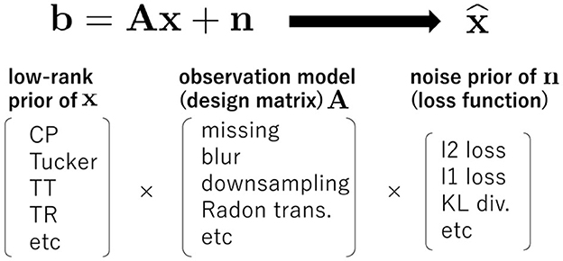
Figure 2. General form of tensor reconstruction problem. Depending on various constraints as low-rank tensors on x, various design matrices A, and various statistical properties of the noise component n, a wide variety of optimization problems can be considered. Low-rank tensor completion and robust tensor decomposition are just a few of them, and considering these problems will enable a wider range of applications.

Furthermore, we consider a penalized version as follow:

$\begin{array}{ll}\underset{\text{x}}{\text{minimize}}D(\text{b},\text{A}\text{x})+i_{𝕊}(\text{x})+\alpha p(\theta ),& (37)\end{array}$

where α ≥ 0 and p(θ) is a penalty function for core tensors θ = ($G$₁, $G$₂, ..., $G$_L). This is a generalization of the problem in Equation 36, since Equation 37 with α = 0 is equivalent to Equation 36. This plays an important role for the introduction of Tikhonov regularization, sparse regularization, low-rank regularization (e.g., nuclear norm), and smoothing. In particular, Tikhonov regularization of the core tensors reduces the problem of non-uniqueness of scale and improves the convergence of the TD algorithm [88].

3 Proposed method

3.1 Sketch of optimization framework

The key idea to solve a diverse set of problems formulated in Equation 36 is to employ the plug-and-play (PnP) approach of TD algorithms such as EM-ALS and ADMM. In this study, we first solve the case of ℓ₂ loss using LS-based TD with the MM framework, which is a generalization of EM-ALS. Furthermore, we use it to solve the cases of ℓ₁ loss and KL divergence with the ADMM framework. Thus, we call the proposed algorithm ADMM-MM. By replacing the LS-based TD module in a PnP manner, various types of TD can be easily generalized and applied to various applications.

3.2 Optimization

In this section, we explain one-by-one how to optimize the problem in Equation 37 for three loss functions: ℓ₂ loss, ℓ₁ loss, and generalized KL divergence. Then, we explain how to combine these three cases as the ADMM-MM algorithm.

3.2.1 Preliminary of LS-based TD

Key module in ADMM-MM is LS-based TD. In vector formulation x instead of $X$, the ALS algorithm of LS-based TD for v = vec($V$) is denoted as

$\begin{array}{l}{\text{argmin}}_{\text{x}}\parallel \text{v}-\text{x}{\parallel }_2^2+i_{𝕊}(\text{x})\\ \approx {\text{Proj}}_{𝕊}^{\text{ALS}}(\text{v},{\text{x}}_0):={\mathcal{U}}_{\text{v},𝕊}^{\text{ALS}}◦\cdots ◦{\mathcal{U}}_{\text{v},𝕊}^{\text{ALS}}({\text{x}}_0),& (38)\end{array}$

where ${\mathrm{\text{Proj}}}_{𝕊}^{\mathrm{\text{ALS}}}$, ${\mathcal{U}}_{\mathbf{\text{v}},𝕊}^{\mathrm{\text{ALS}}}$ and x₀ correspond to ${\mathrm{\text{Proj}}}_{{𝕊}_t}^{\mathrm{\text{ALS}}}$, ${\mathcal{U}}_{V,{𝕊}_t}^{\mathrm{\text{ALS}}}$ and $X$₀, respectively.

Note that ${\mathrm{\text{Proj}}}_{𝕊}^{\mathrm{\text{ALS}}}$ and ${\mathcal{U}}_{\mathbf{\text{v}},𝕊}^{\mathrm{\text{ALS}}}$ do not necessarily have to be strictly based on ALS, and may be replaced by hierarchical ALS (HALS) for CPD [89] or multiplicative update rule for non-negative matrix factorization (NMF) [11, 53]. Furthermore, we aim to solve the penalized version of LS-based TD. In this study, we assume existence of iterative penalized LS-based TD algorithm that minimizes the squared error with penalty, and we denote more general LS-based TD as

$\begin{array}{l}{\text{argmin}}_{\text{x}}\parallel \text{v}-\text{x}{\parallel }_2^2+i_{𝕊}(\text{x})+\alpha p(\theta )\\ \approx {\text{Proj}}_{{𝕊}_{\alpha }}(\text{v},{\text{x}}_0):={\mathcal{U}}_{\text{v},{𝕊}_{\alpha }}◦\cdots ◦{\mathcal{U}}_{\text{v},{𝕊}_{\alpha }}({\text{x}}_0).& (39)\end{array}$

It should be noted that the above LS-based TD algorithm is expressed from the perspective of updating x(θ), however, the core tensors θ = ($G$₁, $G$₂, ..., $G$_L) are also actually updated in practical implementation. In other words, in this algorithm, x and θ are always considered a pair. For simplicity, we will not write it explicitly, but the input to ${\mathcal{U}}_{\mathbf{\text{v}},{𝕊}_{\alpha }}$ requires not only x₀ but also θ₀.

3.2.2 MM for ℓ₂ loss

Here, we consider a case to minimize ℓ₂ loss in Equation 37 as

$\begin{array}{ll}f(\text{x})=\parallel \text{b}-\text{A}\text{x}{\parallel }_2^2+i_{𝕊}(\text{x})+\alpha p(\theta ).& (40)\end{array}$

To minimize f(x), we propose to employ MM approach:

$\begin{array}{ll}{\text{x}}_{k+1}=\underset{\text{x}}{\text{argmin }}g(\text{x}|{\text{x}}_k),& (41)\end{array}$

where auxiliary function g(x|x_k) is given by

$\begin{array}{ll}g(\text{x}|{\text{x}}_k):=f(\text{x})+{(\text{x}-{\text{x}}_k)}^{\top }(\lambda \text{I}-{\text{A}}^{\top }\text{A})(\text{x}-{\text{x}}_k)& (42)\end{array}$

$\begin{array}{l}=\lambda {\displaystyle \parallel \text{x}-\left({\text{x}}_k-\frac{1}{\lambda }({\text{A}}^{\top }\text{A}{\text{x}}_k-{\text{A}}^{\top }\text{b})\right){\parallel }_2^2+i_{𝕊}(\text{x})}\\ +\alpha p(\theta )+\text{const}.& (43)\end{array}$

From Equation 42, the auxiliary function satisfies the conditions of Equation 16 when λ is greater than the maximum eigenvalue of A^⊤A. Then, the MM step in Equation 41 can be reduced to

$\begin{array}{ll}{\text{v}}_k={\text{x}}_k-\frac{1}{\lambda }({\text{A}}^{\top }\text{A}{\text{x}}_k-{\text{A}}^{\top }\text{b});& (44)\end{array}$

$\begin{array}{ll}{\text{x}}_{k+1}={\text{Proj}}_{{𝕊}_{\frac{\alpha }{\lambda }}}({\text{v}}_k,{\text{x}}_k);& (45)\end{array}$

Note that the penalty parameter for LS-based TD becomes $\frac{\alpha }{\lambda }$, and we set λ to be the maximum eigenvalue of A^⊤A in practice.

3.2.3 ADMM for other loss functions

Next, we consider the problem in Equation 37 for other loss functions and propose to employ ADMM as Zhang and Ding's formulation [85]. First, we introduce a new variable y ∈ ℝ^J and a linear constraint y = Ax, and its augmented Lagrangian is given by

$\begin{array}{ll}\mathcal{L}(\text{x},\text{y},\text{z})=D(\text{b},\text{y})+i_{𝕊}(\text{x})+\alpha p(\theta )+\langle \text{z},\text{y}-\text{A}\text{x}\rangle +\frac{\beta }{2}\parallel \text{y}-\text{A}\text{x}{\parallel }_2^2,& (46)\end{array}$

where z ∈ ℝ^J is a Lagrange multiplier and β > 0 is a hyperparameter. In each step of ADMM, x is updated as a minimizer of $\mathcal{L}(\mathbf{\text{x}},\mathbf{\text{y}},\mathbf{\text{z}})$ with respect to x, y is updated as a minimizer of $\mathcal{L}(\mathbf{\text{x}},\mathbf{\text{y}},\mathbf{\text{z}})$ with respect to y, and z is updated by the method of multipliers. ADMM algorithm is given by

$\begin{array}{ll}{\text{x}}_{k+1}=\underset{\text{x}}{\text{argmin}}{i}_{𝕊}(\text{x})+\alpha p(\theta )+\frac{\beta }{2}{\displaystyle \parallel {\text{y}}_k+\frac{{\text{z}}_k}{\beta }-\text{A}\text{x}{\parallel }_2^2;}& (47)\end{array}$

$\begin{array}{ll}{\text{y}}_{k+1}=\underset{\text{y}}{\text{argmin}}D(\text{b},\text{y})+\frac{\beta }{2}{\displaystyle \parallel \text{y}+\frac{{\text{z}}_k}{\beta }-\text{A}{\text{x}}_{k+1}{\parallel }_2^2;}& (48)\end{array}$

$\begin{array}{ll}{\text{z}}_{k+1}={\text{z}}_k+\beta ({\text{y}}_{k+1}-\text{A}{\text{x}}_{k+1});& (49)\end{array}$

where initializations x₀, y₀ and z₀ are required.

3.2.3.1 Update rule for x

Here, we consider practical process in Equation 47. Since ${\mathbf{\text{y}}}_k+\frac{{\mathbf{\text{z}}}_k}{\beta }$ is constant and i_𝕊(x) is invariant to scaler, the structure of Equation 47 is the same as in Equation 40. By using MM approach, update rule in Equation 47 can be replaced with

$\begin{array}{ll}{\text{v}}_k={\text{x}}_k-\frac{1}{\lambda }\left({\text{A}}^{\top }\text{A}{\text{x}}_k-{\text{A}}^{\top }\left({\text{y}}_k+\frac{{\text{z}}_k}{\beta }\right)\right);& (50)\end{array}$

$\begin{array}{ll}{\text{x}}_{k+1}={\text{Proj}}_{{𝕊}_{\frac{2\alpha }{\lambda \beta }}}({\text{v}}_k,{\text{x}}_k);& (51)\end{array}$

Note that the penalty parameter for LS-based TD becomes $\frac{2\alpha }{\lambda \beta }$.

3.2.3.2 Update rule for y

Update rule in Equation 48 is derived depending on the loss function D(b, y). Many loss functions take the form of a sum of entry-wise losses $D(\mathbf{\text{b}},\mathbf{\text{y}})=\sum _{j=1}^{J}d(b_j,y_j)$, in which case the subproblem for updating y is separable for each entry y_j as

$\begin{array}{ll}{y}_j^{*}=\underset{y_j}{\text{argmin}}d(b_j,y_j)+\frac{\beta }{2}{(d_j-y_j)}^2,& (52)\end{array}$

where we put $\mathbf{\text{d}}={\left[d_1,d_2,...,d_J\right]}^{\top }=\mathbf{\text{A}}{\mathbf{\text{x}}}_{k+1}-\frac{{\mathbf{\text{z}}}_k}{\beta }$. The solution in Equation 52 is unique if d(b_j, y_j) is convex. Our algorithm is possible to support loss functions that the problems formulated in Equation 52 have closed-form solutions. Combettes and Pesquet [90] and Parikh and Boyd [91] can be useful for obtaining solutions to several distance functions d(b_j, y_j). For example, when we consider ℓ₁ loss d(b_j, y_j) = |b_j − y_j|, the solution can be given by soft-thresholding as

$\begin{array}{ll}{y}_j^{*}=b_j+{\text{soft}}_{\frac{1}{\beta }}[d_j-b_j].& (53)\end{array}$

When we consider generalized KL divergence for positive y_j > 0 as $d(b_j,y_j)=b_{j}log\frac{b_j}{y_j}+y_j-b_j$, the solution can be given by

$\begin{array}{ll}{y}_j^{*}=\frac{\beta d_j-1+\sqrt{{(\beta d_j-1)}^2+4\beta b_j}}{2\beta }.& (54)\end{array}$

3.3 Proposed algorithm

Finally, the proposed ADMM-MM algorithm that supports three typical loss functions can be summarized in Algorithm 1. Our ADMM-MM allows for the immediate application of sophisticated TD models to other tasks such as completion, robust reconstruction, and compressive sensing. By simply selecting the update rule in the 7th line, we can accommodate the three loss functions. The majorization step on the 9th line is important to allow for accommodating a variety of design matrices A. Many LS-based TD with penalty can be applied into the ADMM-MM algorithm in a plug-and-play manner at the 10th line. The basic expectation of plug-and-play module, Proj_𝕊γ(v, x) or ${\mathcal{U}}_{\mathbf{\text{v}},{𝕊}_{\gamma }}(\mathbf{\text{x}})$, is that it has a monotonically decreasing property with respect to the penalized squared error shown in Equation 39. Note that our algorithm can also involve tensor nuclear norm regularization [65] although not a direct tensor decomposition. That is, a proximal mapping given in closed form of nuclear norm regularization can be replaced directly with Proj_𝕊γ(v, x).

Algorithm 1

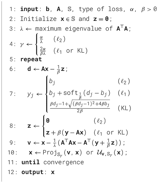
Algorithm 1. ADMM-MM algorithm.

The proposed algorithm can be regarded as a unified and extended algorithm of EM-ALS and Zhang and Ding's ADMM. When A is the diagonal matrix of vectorization of the mask tensor $W$ (e.g., A = diag(vec($W$))) and ℓ₂ loss is assumed, the ADMM-MM algorithm results in EM-ALS. When A = I and ℓ₁ loss is assumed, the ADMM-MM algorithm results in Zhang and Ding's ADMM.

From the perspective of an optimization algorithm that uses ADMM with MM, the proposed algorithm can be regarded as a special case of linearized ADMM [92, 93]. However, the linearized ADMM work [92] considers only convex optimizations, while the other work [93] considers only non-convex matrix norms which have effective proximal mappings. The major difference in the proposed method from the above methods is that the update rule of the iterative algorithm is applied to penalized TD instead of proximal mapping. Our proposal to plug-and-play various TDs is a new and meaningful attempt, which will greatly improve the applicability of TDs.

The computational complexity of a single iteration in the ADMM-MM algorithm is often dominated by the LS-based TD at the 10th line. The complexity of lines 6 through 9 is $\mathcal{O}(\Omega )$, where Ω is the number of nonzero elements in the design matrix A ∈ ℝ^{J × I}. We often assume that the design matrix is sparse and J ≤ Ω ≪ IJ. On the other hand, the complexity of LS-based TD for N-th order tensor $V$ ∈ ℝ^{I₁ × I₂ × ⋯ × I_N} depends on the model and algorithm. CPD/NNCPD can be solved by ALS and HALS [2, 8]. The complexity of CP-ALS is $\mathcal{O}(NI{R}_{\mathrm{\text{CP}}})+\mathcal{O}(N{R}_{\mathrm{\text{CP}}}^3)$, while the complexity of HALS is $\mathcal{O}(NI{R}_{\mathrm{\text{CP}}})$, assuming that the CP rank is denoted as R_CP and $I={\prod }_{i=1}^N{I}_i$. ALS is computationally more expensive than HALS because it requires matrix inversion. TKD is usually solved by the higher-order orthogonal iteration (HOOI) algorithm [48], which solves N eigenvalue problems alternately. Since the symmetric matrix of size (I_n, I_n) by tensor-matrix multiplication is usually more expensive than its eigenvalue problem, then the complexity of HOOI is $\mathcal{O}(NI{R}_{\mathrm{\text{TK}}})$, assuming that the Tucker rank is (R_TK, R_TK, ..., R_TK). TTD is usually solved by TT-ALS with QR orthogonalization [50]. The advantage of this algorithm is that QR orthogonalization allows each least-squares solution to be found without matrix inversion. The complexity of TT-ALS is $\mathcal{O}(NI{R}_{\mathrm{\text{TT}}})$, assuming that the TT-rank is (R_TT, R_TT, ..., R_TT). TRD is usually solved by TR-ALS [51]. The complexity of TR-ALS is $\mathcal{O}(NI{R}_{\mathrm{\text{TR}}}^2)+\mathcal{O}(N{R}_{\mathrm{\text{TR}}}^6)$, assuming that the TR-rank is (R_TR, R_TR, ..., R_TR). From a complexity perspective, TKD and TTD are highly efficient. TRD has a higher complexity with respect to TR rank. CPD often requires a larger CP rank, making it more expensive than other models.

3.4 Discussions on the convergence

Unfortunately, this study does not include new theoretical results on the convergence of the ADMM-MM algorithm using Ls-based TD algorithms for sub-optimization. Instead, this section introduces existing theoretical results on convergence related to TD, EM/MM, and ADMM, and discusses their relevance to this study.

3.4.1 Case of ℓ₂ loss with MM

The theory of monotonicity and convergence of the EM and MM algorithms has been discussed [83, 94], and global convergence has been shown when the minimizer of the auxiliary function is unique [95]. In this study, ALS and MM are combined for ℓ₂ loss minimization. From a point of view of only MM, the results of MM [95] cannot be applied to our case since our auxiliary function is non-convex and its minimizer is not unique in general. On the other hand, the convergence of tensor completion via non-negative tensor factorization [96] has been studied, which corresponds to a special case of our algorithm.

In Section 3.2.2, we explain the proposed MM algorithm, which first derives the auxiliary function and then minimizes it using ALS (or BCD). However, the same auxiliary function and algorithm can be derived by considering the opposite way which first considers to minimize the original function using ALS (or BCD) and then derives the auxiliary function for each sub-optimization problem. From this perspective, the proposed algorithm for ℓ₂ loss is included in a framework named block majorization minimization or block successive upper bound minimization [97, 98]. In short, from the results of convergence [97, 98], the proposed algorithm has global convergence if the auxiliary function of each sub-optimization has a unique minimizer. Although the solution to the sub-optimization in ALS is generally not unique, this can sometimes be resolved by adding regularization. For example, in the case of the use of Tikhonov regularized ALS for sub-optimization, global convergence is guaranteed in the proposed MM algorithm.

3.4.2 Case of other loss with ADMM

When A = I, the proposed algorithm is reduced to the standard ADMM. Usually, the convergence of ADMM is based on the non-expansive property of projection onto a convex set or proximal mapping of a convex function [99], and it can not be applicable to our case since low-rank tensor approximation is characterized as a projection onto a non-convex set, Proj_𝕊, or non-convex sub-optimization, Proj_𝕊γ. As a related work [100], the ADMM algorithm and its convergence for the completion of the matrix with NMF have been discussed, however, in their formulation, each factor matrix of NMF is treated separately as an optimization variable in ADMM, which differs from our formulation. On the other hand, the non-convex ADMM [101] includes many non-convex functions and indicator functions of non-convex sets such as the Stiefel/Grassmannian manifold, and it is close to our problem. According to this theory, the compactness of the set 𝕊, the coercivity and smoothness of the objective function, and the continuity of the sub-optimization paths are required for convergence. It is not trivial whether these conditions apply in our case because Proj_𝕊γ is a composite problem of tensor decomposition and penalization of the core tensors.

When A ≠ I, the proposed algorithm is characterized as ADMM with MM for its sub-optimization. This combination of ADMM and MM is often referred to as linearized ADMM [92]. Non-convex linearized ADMM [93] and its convergence have been discussed, and it is applied to non-convex low-rank matrix reconstruction problem. However, it is not trivial whether the results of convergence [93] can be applied in our case. From the perspective of PnP-ADMM, the results of the convergence analysis based on the Lipschitz condition of the denoiser have been reported [102]. Thus, although there are various relevant results, whether they apply specifically to our case is an open problem. This open problem may be solved by analyzing the properties of the penalized TD algorithm.

4 Related works

There are several studies on algorithms for TD using ADMM. AO-ADMM [73] is an algorithm for constrained matrix/tensor factorization which solves the sub-problems for updating factor matrices using ADMM. Although alternating optimization (AO) is the main-routine and ADMM is subroutine in AO-ADMM, in contrast, the proposed ADMM-MM algorithm is ADMM is used as main-routine. AO-ADMM supports several loss functions, but it does not support various design matrices. In addition, AO-PDS [103] has been proposed using primal-dual splitting (PDS) instead of ADMM.

Robust Tucker decomposition (RTKD) with ℓ₁ loss has been proposed [85] and its algorithm has been developed based on ADMM. RTKD employs ADMM as the main routine, ALS is used as the subroutine, and it can be regarded as a special case of our proposed algorithm. RTKD does not support any other loss function, various design matrices, and other constraints.

The penalized TD using ADMM has been actively studied and many algorithms have been proposed [100, 104–107]. Each of these algorithms is a detailed formulation of ADMM tailored to the problem, and the optimization variables are separated into many blocks and updated alternately. The algorithms are not structured, making them difficult to generalize and extend.

In the context of generalized TD, generalized CPD [108] has been proposed. The purpose of the study is to make the CP decomposition compatible with various loss functions. Basically, a BCD-based gradient algorithm has been proposed. However, other TD models and perspectives on design matrices are not discussed.

PnP-ADMM [54] is a framework for using some black-box models (e.g., trained deep denoiser) instead of proximal mapping in ADMM. It is highly extensible, in that any model can be applied to various design matrices. The structure of using LS-based TD in a plug-and-play manner in the proposed algorithm is basically the same as that of PnP-ADMM. If we consider LS-based TD as a denoiser, the proposed algorithm may be considered a type of PnP-ADMM. In this sense, the proposed algorithm and PnP-ADMM are very similar, but they are significantly different in that our objective function is not a black box.

5 Experiments

The purpose of the experiments is to evaluate the performance of the proposed algorithm in terms of optimization and to investigate its usefulness for versatile tensor reconstruction tasks.

5.1 Optimization behaviors for various tensor reconstruction tasks

Tensor reconstruction tasks in this experiment include tensor denoising, completion, de-blurring, and super-resolution. We used an RGB image named “facade” represented as a third-order tensor of size 256 × 256 × 3 for ground truth in denoising, completion, de-blurring, and super-resolution tasks.

For tensor denoising task, we set A = I. Gaussian noise, salt-and-pepper noise, and Poisson noise are added for individual tasks. For tensor completion tasks, we set A = diag(vec($W$)) with a randomly generated mask tensor $W$ ∈ {0, 1}^{256 × 256 × 3}, where 90% of the entries are missing. For de-blurring tasks, we used a motion blur window of size 21 × 21, and the constructed block Toeplitz matrix is used as A. For super-resolution tasks, we used a Lanczos2 kernel for downsampling to 1/4 size, and the constructed downsampling matrix is used as A.

5.1.1 Comparison with gradient methods

In this experiment, we compare the proposed algorithm with two gradient-based algorithms: projected gradient (PG) and block coordinate descent (BCD) with the low-rank CP decomposition model:

$\begin{array}{ll}\text{x}=\text{vec}(⟦{\text{G}}^{(1)},{\text{G}}^{(2)},{\text{G}}^{(3)}⟧)\in 𝕊\subset {ℝ}^{256·256·3},& (55)\end{array}$

$\begin{array}{l}𝕊:\text{}=\{\text{vec}(〚G^{(1)},G^{(2)},G^{(3)}〛)|G^{(1)}\in {ℝ}^{256\times R},G^{(2)}\in {ℝ}^{256\times R},\\ G^{(3)}\in {ℝ}^{3\times R}\}.& (56)\end{array}$

In PG, x is moved along the gradient descent direction and then projected onto the set 𝕊.

$\begin{array}{ll}{\text{v}}_k={\text{x}}_k-\mu {\nabla }_{\text{x}}D(\text{b},\text{A}{\text{x}}_k);& (57)\end{array}$

$\begin{array}{ll}{\text{x}}_{k+1}={\text{Proj}}_{𝕊}^{\text{ALS}}({\text{v}}_k,{\text{x}}_k);& (58)\end{array}$

where μ > 0 is a step-size. Note that it is the same as the proposed method when $D(\mathbf{\text{b}},\mathbf{\text{ A}}\mathbf{\text{x}})=\parallel \mathbf{\text{b}}-\mathbf{\text{A}}\mathbf{\text{x}}{\parallel }_2^2$ and $\mu =\frac{1}{\lambda }$. In BCD based gradient algorithm is given by

$\begin{array}{ll}{\text{G}}_{k+1}^{(1)}={\text{G}}_k^{(1)}-\mu {\nabla }_{{\text{G}}^{(1)}}D(\text{b},\text{A}\text{vec}(⟦{\text{G}}_k^{(1)},{\text{G}}_k^{(2)},{\text{G}}_k^{(3)}⟧));& (59)\end{array}$

$\begin{array}{ll}{\text{G}}_{k+1}^{(2)}={\text{G}}_k^{(2)}-\mu {\nabla }_{{\text{G}}^{(2)}}D(\text{b},\text{A}\text{vec}(⟦{\text{G}}_{k+1}^{(1)},{\text{G}}_k^{(2)},{\text{G}}_k^{(3)}⟧));& (60)\end{array}$

$\begin{array}{ll}{\text{G}}_{k+1}^{(3)}={\text{G}}_k^{(3)}-\mu {\nabla }_{{\text{G}}^{(3)}}D(\text{b},\text{A}\text{vec}(⟦{\text{G}}_{k+1}^{(1)},{\text{G}}_{k+1}^{(2)},{\text{G}}_k^{(3)}⟧));& (61)\end{array}$

In both PG and BCD, step-size μ was manually adjusted for the best performance. The proposed algorithm has an optimization parameter β and was also manually adjusted. We experimented with four tasks of denoising, completion, de-blurring and super-resolution under Gaussian, salt-and-pepper, and Poisson noise measurement. ℓ₂ loss, ℓ₁ loss, and generalized KL divergence are used for Gaussian, salt-and-pepper, and Poisson noise measurements, respectively.

Table 1 shows the achieved values of the objective function and its computational time [sec] for the three optimization methods in various settings. The best values are highlighted in bold. Figure 3 shows its optimization behaviors in the various tasks based on three loss functions. The proposed method stably and efficiently reduces the objective function in various settings in comparison to PG and BCD. Note that since the proposed method for ℓ₂ loss and PG are equivalent, they are not compared.

Table 1

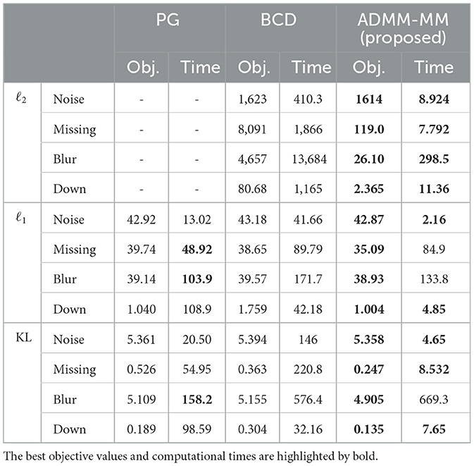
Table 1. Comparison of objective functions and computational time [sec] at convergence for PG, BCD, and the proposed algorithms.

Figure 3

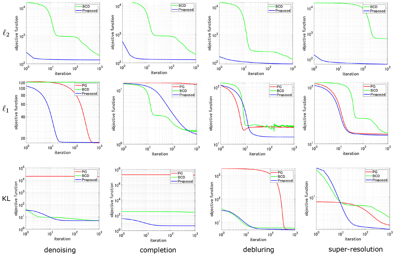
Figure 3. Optimization behavior: comparison of PG, BCD, and the proposed algorithm for various loss functions in CP decomposition with various degraded images.

5.1.2 Comparison with AO-ADMM

In this experiment, we compare the proposed method with AO-ADMM in standard non-negative CP decomposition (NNCPD) under three loss functions. The optimization problem is given by

$\begin{array}{r}\underset{{\text{G}}^{(1)},{\text{G}}^{(2)},{\text{G}}^{(3)}}{\text{minimize}}D(\text{b},\text{vec}(⟦{\text{G}}^{(1)},{\text{G}}^{(2)},{\text{G}}^{(3)}⟧)),\text{ s.t. }{\text{G}}^{(1)}\in {ℝ}_{\ge 0}^{256\times R},\\ {\text{G}}^{(2)}\in {ℝ}_{\ge 0}^{256\times R},{\text{G}}^{(3)}\in {ℝ}_{\ge 0}^{3\times R},& (62)\end{array}$

where ℝ_≥0 is a set of non-negative real numbers. In AO-ADMM, each G^(l) is updated by sub-optimization using ADMM. We used the original implementation of AO-ADMM by Huang¹ with some modifications to adopt it for the TD problem. In the proposed method, we plug-and-played the multiplicative update (MU) [11] and the hierarchical alternating least squares (HALS) [89] for LS-based NNCPD.

Figure 4 and Table 2 show the comparison of the convergence behaviors between the proposed method and the AO-ADMM. We experimented with weak and strong noise setting under three types of noise. The value displayed below each plot represents the signal-to-noise ratio (SNR) of noisy measurements. Although the MU and HALS used in plug-and-play are not pure least squares minimizers, we can see that they successively converged. In the early stages of optimization, the objective function decreased faster with AO-ADMM, but there were no significant differences in the convergence speed. When comparing the time to convergence, AO-ADMM was slightly faster to minimize ℓ₂ loss, while the proposed method was slightly faster to minimize ℓ₁ loss and generalized KL divergence.

Figure 4

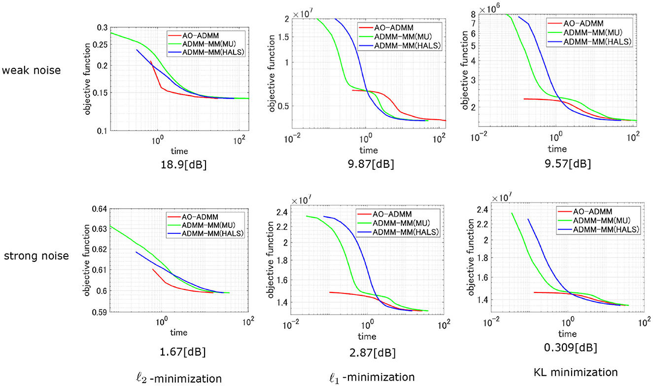
Figure 4. Comparison of the convergence behavior of the AO-ADMM and the proposed method. Non-negative CP decomposition is performed under three loss functions. Observations are varied with two different noise levels.

Table 2

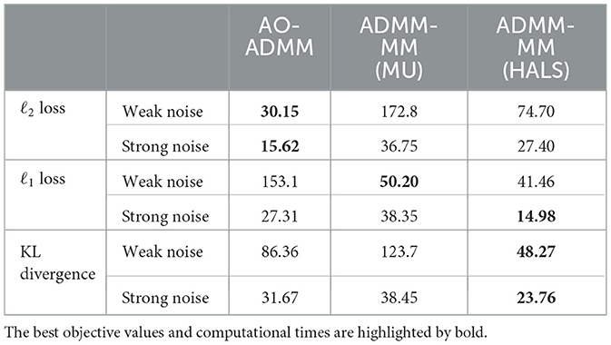
Table 2. Comparison of the time required for the objective function to converge in noise removal using AO-ADMM and ADMM-MM.

It should be noted that it is difficult to make a fair comparison of the convergence of the AO-ADMM and ADMM-MM algorithms. AO-ADMM has an AO main-iteration and an ADMM sub-iteration for sub-problems, making it a double-loop algorithm. In this study, 10 sub-iterations were performed, but changing this may change the convergence results. Also the convergence behavior changes significantly depending on the parameter β in ADMM. The appropriate beta value differs depending on the task, loss function, and model.

5.1.3 Various tensor decomposition models

Here, we apply the proposed ADMM-MM algorithm to four types of TD models: CP, Tucker, TT, and TR decompositions. The standard ALS algorithm is used for CP and TR decompositions [42, 43, 51], and orthogonalized ALS is used for Tucker and TT decompositions [48, 50].

Figure 5 shows the selected results, and various tensor reconstruction settings for all TD models can be succinctly optimized by the proposed ADMM-MM algorithm.

Figure 5

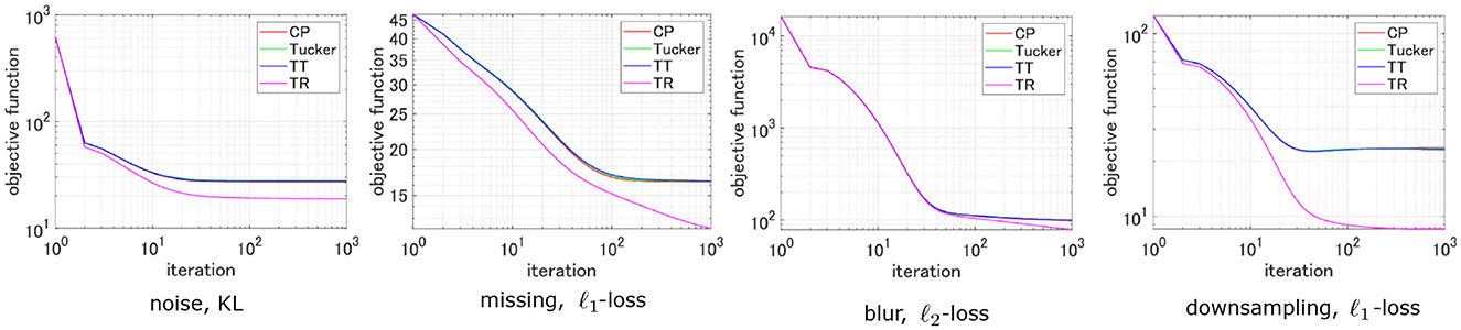
Figure 5. Comparison of cost function convergence in various TD models across different design matrices and loss functions.

5.1.4 Sensitivity of a hyperparameter β

Here, we show the differences in convergence behaviors of ADMM-MM algorithm with respect to the values of hyperparameter β. In this experiment, the tensor completion task was solved using the ALS algorithm of CP decomposition with Tikhonov regularization. β is a hyperparameter related to ADMM, so there are two settings: minimizing ℓ₁ loss and KL divergence. Figure 6 shows the convergence behaviors of the loss function obtained with various values of β. Similar trends were obtained for both loss functions. When β is large, it is stable but convergence is slow. Making β smaller will speed up the convergence, but if it is too small, the convergence becomes unstable.

Figure 6

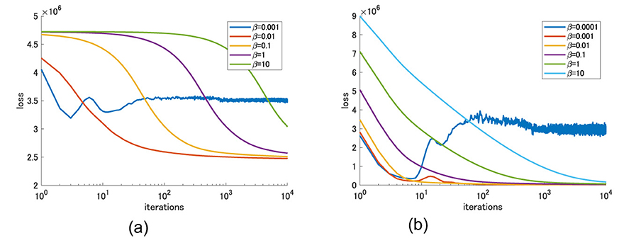
Figure 6. Convergence behaviors with respect to hyperparameter β. (a) l1-loss. (b) KL divergence.

5.2 Image processing applications

In this experiment, we demonstrate that the proposed algorithm connects various TD models with various image processing tasks.

5.2.1 Color image reconstruction and computed tomography

Here, we show the results of color image reconstruction and computed tomography using the proposed ADMM-MM algorithm. An RGB image named “facade” is used for three image-inpainting tasks under three different noises (tasks 1, 2, and 3) and for an image deblurring task under sparse noise (task 4). An artificial low-rank tensor of size 128 × 128 × 3 is used for computed tomography under Poisson noise (task 5).

We apply various TD models for various image reconstruction tasks to demonstrate the potential of the proposed method. We used six TD models: CP decomposition (CPD), Tucker decomposition (TKD), TR decomposition (TRD) [51], tensor nuclear norm regularization (tSVD) [65], NNCP decomposition (NNCPD) [12], and smooth PARAFAC (SPC) [34]. tSVD stands for tensor nuclear norm regularization using singular value shresholding. NNCPD stands for CP decomposition with non-negative constraints of factor matrices. Each factor matrices are updated by multiplicative update rules. SPC stands for CP decomposition with smoothness constraints of factor matrices. Although the SPC has been originally proposed for LS-based tensor completion, our framework can extend it to ℓ₁ loss and KL-divergence with arbitrary design matrix A.

Figure 7 shows the results obtained by six TD models in image processing tasks: tensor completion under Gaussian noise (task 1), tensor completion under sparse noise (task 2), tensor completion under Poisson noise (task 3), de-blurring under sparse noise (task 4), and computed tomography under Poisson noise (task 5). We can see that the proposed method allows to plug-and-play many TD models for application to a variety of image processing tasks.

Figure 7

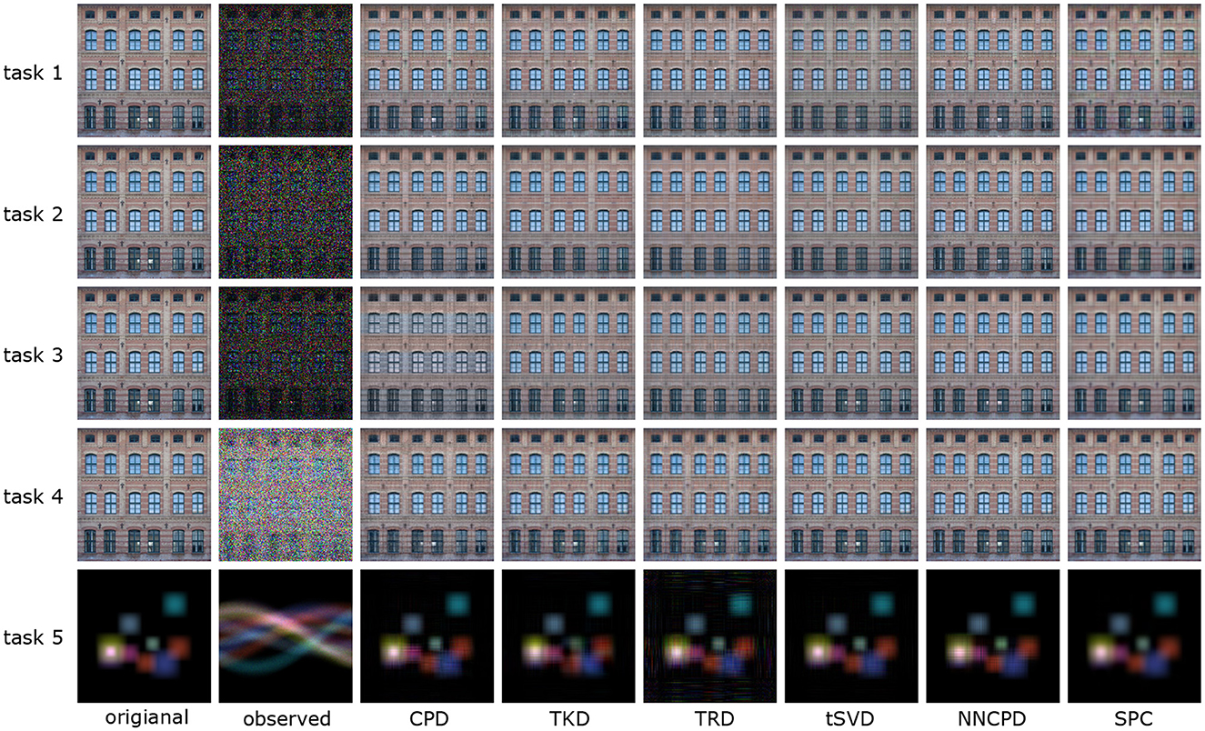
Figure 7. Reconstruction of various degraded images using the proposed method with different tensor decomposition approaches.

5.2.2 Application to light field image recovery

Here, we apply the proposed algorithm to the problem of light field image restoration as one of the case studies. The light field image used is a fourth-order tensor named “vinyl” with size (128,128,3,81).² An algorithm for light field image restoration under the hybrid model of Tucker and TT decompositions, named fast tensor train nuclear norm (FTTNN),³ has been studied [109]. The task is to restore the original image from an image in which 20% of the pixels are randomly selected and overwritten with random values.

Our framework allows us to apply different kinds of TD model to this task and compare them with the existing algorithm. Table 3 shows the results of the comparison with PSNR, RSE, and SSIM metrics. We applied TKD, TTD, TRD, CPD, NNCPD, and SPC to this task by using the proposed ADMM-MM algorithm. In particular, we were able to demonstrate a high level of performance with the constrained CPD models ( i.e., NNCPD and SPC) in light field image recovery.

Table 3

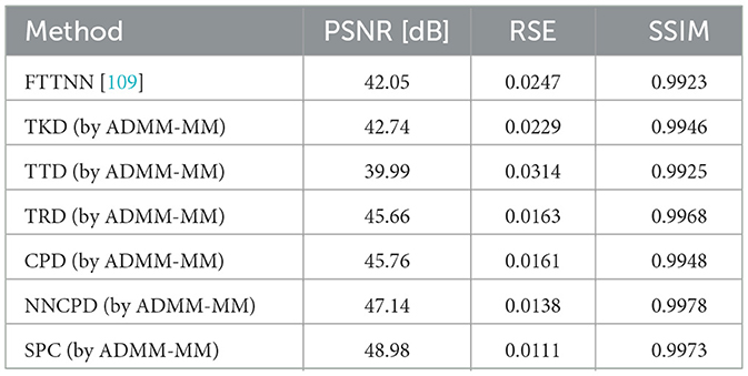
Table 3. Comparison of TD models with PSNR, RSE, and SSIM metrics in light field image recovery.

6 Conclusion

In this study, we proposed a versatile tensor reconstruction framework to plug-and-play various LS-based TD algorithms and apply them to various applications. This framework is very practical because many TD models are often initially studied on the basis of least squares. The newly proposed TD algorithm can be plug-and-played and operated based on any design matrix and at least three loss functions. In addition, any loss function having a proximal mapping can be easily introduced.

In experiments, we demonstrated the effectiveness of the proposed method compared to existing gradient-based optimization algorithms and AO-ADMM. Although the convergence of the proposed algorithm is theoretically ambiguous, experimentally we confirmed that it has been successfully optimized for various problems, models, and hyperparameter settings. It was also demonstrated that it is useful for a wide range of image processing applications.

In this study, we plug-and-played various TD algorithms and confirmed their effectiveness, but it would be meaningful to investigate a class of tensor decomposition algorithms that can be plug-and-played by theoretical analysis. Furthermore, there are some properties, such as convergence, that remain unclear, so continued investigation is necessary. In addition, it would also be worthwhile to conduct a study on ways to accelerate the convergence of the algorithm.

Data availability statement

Publicly available datasets were analyzed in this study. This data can be found here: https://github.com/yokotatsuya/PnP-Tensor-Decomposition.

Author contributions

MM: Writing – review & editing, Writing – original draft. HH: Writing – review & editing. TY: Writing – original draft, Writing – review & editing.

Funding

The author(s) declare that financial support was received for the research and/or publication of this article. This work was partially supported by the Japan Society for the Promotion of Science (JSPS) KAKENHI under Grant 23K28109.

Conflict of interest

The authors declare that the research was conducted in the absence of any commercial or financial relationships that could be construed as a potential conflict of interest.

Generative AI statement

The author(s) declare that Gen AI was used in the creation of this manuscript. We used generative AI to proofread the English in the manuscript.

Any alternative text (alt text) provided alongside figures in this article has been generated by Frontiers with the support of artificial intelligence and reasonable efforts have been made to ensure accuracy, including review by the authors wherever possible. If you identify any issues, please contact us.

Publisher's note

All claims expressed in this article are solely those of the authors and do not necessarily represent those of their affiliated organizations, or those of the publisher, the editors and the reviewers. Any product that may be evaluated in this article, or claim that may be made by its manufacturer, is not guaranteed or endorsed by the publisher.

Footnotes

1. ^https://www.cise.ufl.edu/~kejun/code.html

2. ^Data is available online: https://lightfield-analysis.uni-konstanz.de/.

3. ^Code is available online: https://github.com/ynqiu/fast-TTRPCA.

References

1. Yokota T, Caiafa CF, Zhao Q. Tensor methods for low-level vision. In:Liu Y, , editor. Tensors for Data Processing: Theory, Methods, and Applications. Academic Press Inc Elsevier Science (2021). p. 371–425. doi: 10.1016/B978-0-12-824447-0.00017-0

Crossref Full Text | Google Scholar

2. Cichocki A, Zdunek R, Phan AH, Amari SI. Nonnegative Matrix and Tensor Factorizations: Applications to Exploratory Multi-Way Data Analysis and Blind Source Separation. New York: John Wiley & Sons, Ltd. (2009). doi: 10.1002/9780470747278

Crossref Full Text | Google Scholar

3. Li L, Li Y, Li Z. Efficient missing data imputing for traffic flow by considering temporal and spatial dependence. Transport Res Part C. (2013) 34:108–20. doi: 10.1016/j.trc.2013.05.008

Crossref Full Text | Google Scholar

4. Chen H, Ahmad F, Vorobyov S, Porikli F. Tensor decompositions in wireless communications and MIMO radar. IEEE J Sel Top Signal Process. (2021) 15:438–53. doi: 10.1109/JSTSP.2021.3061937

Crossref Full Text | Google Scholar

5. Kalev A, Kosut RL, Deutsch IH. Quantum tomography protocols with positivity are compressed sensing protocols. NPJ Quant Inf . (2015) 1:1–6. doi: 10.1038/npjqi.2015.18

Crossref Full Text | Google Scholar

6. Kyrillidis A, Kalev A, Park D, Bhojanapalli S, Caramanis C, Sanghavi S. Provable compressed sensing quantum state tomography via non-convex methods. NPJ Quant Inf . (2018) 4:36. doi: 10.1038/s41534-018-0080-4

Crossref Full Text | Google Scholar

7. Qin Z, Jameson C, Gong Z, Wakin MB, Zhu Z. Quantum state tomography for matrix product density operators. IEEE Trans Inf Theory. (2024) 70:5030–56. doi: 10.1109/TIT.2024.3360951

Crossref Full Text | Google Scholar

8. Kolda TG, Bader BW. Tensor decompositions and applications. SIAM Rev. (2009) 51:455–500. doi: 10.1137/07070111X

Crossref Full Text | Google Scholar

9. Cichocki A, Mandic D, De Lathauwer L, Zhou G, Zhao Q, Caiafa C, et al. Tensor decompositions for signal processing applications: from two-way to multiway component analysis. IEEE Signal Process Mag. (2015) 32:145–63. doi: 10.1109/MSP.2013.2297439

Crossref Full Text | Google Scholar

10. Yokota T. Very basics of tensors with graphical notations: unfolding, calculations, and decompositions. arXiv preprint arXiv:241116094 (2024).

Google Scholar

11. Lee D, Seung HS. Algorithms for non-negative matrix factorization. In: Advances in Neural Information Processing Systems (2000). p. 13.

Google Scholar

12. Cichocki A, Zdunek R, Amari Si. Nonnegative matrix and tensor factorization [lecture notes]. IEEE Signal Process Mag. (2007) 25:142–5. doi: 10.1109/MSP.2008.4408452

Crossref Full Text | Google Scholar

13. Gillis N. Nonnegative Matrix Factorization. London: SIAM (2020). doi: 10.1137/1.9781611976410

Crossref Full Text | Google Scholar

14. Papalexakis EE, Faloutsos C, Sidiropoulos ND. Parcube: Sparse parallelizable tensor decompositions. In: Proceedings of European Conference on Machine Learning and Principles and Practice of Knowledge Discovery in Databases. Springer (2012). p. 521–536. doi: 10.1007/978-3-642-33460-3_39

PubMed Abstract | Crossref Full Text | Google Scholar

15. Yokota T, Cichocki A. Multilinear tensor rank estimation via sparse Tucker decomposition. In: Proceedings of International Conference on Soft Computing and Intelligent Systems (SCIS) and International Symposium on Advanced Intelligent Systems (ISIS). IEEE (2014). p. 478–483. doi: 10.1109/SCIS-ISIS.2014.7044685

Crossref Full Text | Google Scholar

16. Caiafa CF, Cichocki A. Block sparse representations of tensors using Kronecker bases. In: Proceedings of ICASSP. IEEE (2012). p. 2709–2712. doi: 10.1109/ICASSP.2012.6288476

PubMed Abstract | Crossref Full Text | Google Scholar

17. Caiafa CF, Cichocki A. Computing sparse representations of multidimensional signals using Kronecker bases. Neural Comput. (2013) 25:186–220. doi: 10.1162/NECO_a_00385

PubMed Abstract | Crossref Full Text | Google Scholar

18. Essid S, Févotte C. Smooth nonnegative matrix factorization for unsupervised audiovisual document structuring. IEEE Trans Multim. (2012) 15:415–25. doi: 10.1109/TMM.2012.2228474

Crossref Full Text | Google Scholar

19. Yokota T, Zdunek R, Cichocki A, Yamashita Y. Smooth nonnegative matrix and tensor factorizations for robust multi-way data analysis. Signal Proc. (2015) 113:234–49. doi: 10.1016/j.sigpro.2015.02.003

Crossref Full Text | Google Scholar

20. Yokota T, Kawai K, Sakata M, Kimura Y, Hontani H. Dynamic PET image reconstruction using nonnegative matrix factorization incorporated with deep image prior. In: Proceedings of ICCV (2019). p. 3126–3135. doi: 10.1109/ICCV.2019.00322

Crossref Full Text | Google Scholar

21. Takayama H, Yokota T. A new model for tensor completion: smooth convolutional tensor factorization. IEEE Access. (2023) 11:67526–39. doi: 10.1109/ACCESS.2023.3291744

Crossref Full Text | Google Scholar

22. Cai D, He X, Han J, Huang TS. Graph regularized nonnegative matrix factorization for data representation. IEEE Trans Pattern Anal Mach Intell. (2010) 33:1548–60. doi: 10.1109/TPAMI.2010.231

PubMed Abstract | Crossref Full Text | Google Scholar

23. Yin M, Gao J, Lin Z. Laplacian regularized low-rank representation and its applications. IEEE Trans Pattern Anal Mach Intell. (2015) 38:504–17. doi: 10.1109/TPAMI.2015.2462360

PubMed Abstract | Crossref Full Text | Google Scholar

24. Li X, Ng MK, Cong G, Ye Y, Wu Q. MR-NTD manifold regularization nonnegative Tucker decomposition for tensor data dimension reduction and representation. IEEE Trans Neural Netw Learn Syst. (2016) 28:1787–800. doi: 10.1109/TNNLS.2016.2545400

PubMed Abstract | Crossref Full Text | Google Scholar

25. Cai JF, Candes EJ, Shen Z. A singular value thresholding algorithm for matrix completion. SIAM J Optimiz. (2010) 20:1956–82. doi: 10.1137/080738970

Crossref Full Text | Google Scholar

26. Acar E, Dunlavy DM, Kolda TG, Mørup M. Scalable tensor factorizations for incomplete data. Chemometr Intell Lab Syst. (2011) 106:41–56. doi: 10.1016/j.chemolab.2010.08.004

PubMed Abstract | Crossref Full Text | Google Scholar

27. Liu J, Musialski P, Wonka P, Ye J. Tensor completion for estimating missing values in visual data. IEEE Trans Pattern Anal Mach Intell. (2013) 35:208–20. doi: 10.1109/TPAMI.2012.39

PubMed Abstract | Crossref Full Text | Google Scholar

28. Kressner D, Steinlechner M, Vandereycken B. Low-rank tensor completion by Riemannian optimization. BIT Numer Mathem. (2014) 54:447–68. doi: 10.1007/s10543-013-0455-z

Crossref Full Text | Google Scholar

29. Xu Y, Hao R, Yin W, Su Z. Parallel matrix factorization for low-rank tensor completion. Inverse Problems Imag. (2015) 9:601–24. doi: 10.3934/ipi.2015.9.601

Crossref Full Text | Google Scholar

30. Kim YD, Choi S. Weighted nonnegative matrix factorization. In: Proceedings of ICASSP. IEEE (2009). p. 1541–1544. doi: 10.1109/ICASSP.2009.4959890

Crossref Full Text | Google Scholar

31. Nielsen SFV, Mørup M. Non-negative tensor factorization with missing data for the modeling of gene expressions in the human brain. In: Proceedings of IEEE International Workshop on Machine Learning for Signal Processing. IEEE (2014). p. 1–6. doi: 10.1109/MLSP.2014.6958919

Crossref Full Text | Google Scholar

32. Mørup M, Hansen LK, Arnfred SM. Algorithms for sparse nonnegative Tucker decompositions. Neural Comput. (2008) 20:2112–2131. doi: 10.1162/neco.2008.11-06-407

PubMed Abstract | Crossref Full Text | Google Scholar

33. Zhou G, Cichocki A, Zhao Q, Xie S. Efficient nonnegative Tucker decompositions: Algorithms and uniqueness. IEEE Trans Image Proc. (2015) 24:4990–5003. doi: 10.1109/TIP.2015.2478396

PubMed Abstract | Crossref Full Text | Google Scholar

34. Yokota T, Zhao Q, Cichocki A. Smooth PARAFAC decomposition for tensor completion. IEEE Trans Signal Proc. (2016) 64:5423–36. doi: 10.1109/TSP.2016.2586759

PubMed Abstract | Crossref Full Text | Google Scholar

35. Ghalamkari K, Sugiyama M. Fast rank-1 NMF for missing data with KL divergence. In: Proceedings of International Conference on Artificial Intelligence and Statistics. PMLR (2022). p. 2927–2940.

Google Scholar

36. Durand A, Roueff F, Jicquel JM, Paul N. New penalized criteria for smooth non-negative tensor factorization with missing entries. IEEE Trans Signal Proc. (2024). doi: 10.1109/TSP.2024.3392357

Crossref Full Text | Google Scholar

37. Lyu C, Lu QL, Wu X, Antoniou C. Tucker factorization-based tensor completion for robust traffic data imputation. Transp Res Part C. (2024) 160:104502. doi: 10.1016/j.trc.2024.104502

Crossref Full Text | Google Scholar

38. Boyd S, Parikh N, Chu E, Peleato B, Eckstein J. Distributed optimization and statistical learning via the alternating direction method of multipliers. Found Trends Mach Learn. (2011) 3:1–122. doi: 10.1561/2200000016

Crossref Full Text | Google Scholar

39. Hunter DR, Lange K. A tutorial on MM algorithms. Am Stat. (2004) 58:30–7. doi: 10.1198/0003130042836

PubMed Abstract | Crossref Full Text | Google Scholar

40. Sun Y, Babu P, Palomar DP. Majorization-minimization algorithms in signal processing, communications, and machine learning. IEEE Trans Signal Proc. (2016) 65:794–816. doi: 10.1109/TSP.2016.2601299

Crossref Full Text | Google Scholar

41. Hitchcock FL. The expression of a tensor or a polyadic as a sum of products. J Mathem Phys. (1927) 6:164–89. doi: 10.1002/sapm192761164

Crossref Full Text | Google Scholar

42. Carroll JD, Chang JJ. Analysis of individual differences in multidimensional scaling via an N-way generalization of “Eckart-Young” decomposition. Psychometrika. (1970) 35:283–319. doi: 10.1007/BF02310791

Crossref Full Text | Google Scholar

43. Harshman RA. Foundations of the PARAFAC procedure: models and conditions for an “explanatory” multimodal factor analysis. UCLA Work Paper Phonet. (1970) 16:1–84.

Google Scholar

44. Tucker LR. Implications of factor analysis of three-way matrices for measurement of change. Probl Measur Change. (1963) 12:122–137.

Google Scholar

45. Tucker LR. The extension of factor analysis to three-dimensional matrices. Contr Mathem Psychol. (1964) 51:109–127.

Google Scholar

46. Tucker LR. Some mathematical notes on three-mode factor analysis. Psychometrika. (1966) 31:279–311. doi: 10.1007/BF02289464

PubMed Abstract | Crossref Full Text | Google Scholar

47. Kroonenberg PM, De Leeuw J. Principal component analysis of three-mode data by means of alternating least squares algorithms. Psychometrika. (1980) 45:69–97. doi: 10.1007/BF02293599

Crossref Full Text | Google Scholar

48. De Lathauwer L, De Moor B, Vandewalle J. On the best rank-1 and rank-(r_1, r_2, r_n) approximation of higher-order tensors. SIAM J Matrix Analy Applic. (2000) 21:1324–42. doi: 10.1137/S0895479898346995

Crossref Full Text | Google Scholar

49. Oseledets IV. Tensor-train decomposition. SIAM J Sci Comput. (2011) 33:2295–317. doi: 10.1137/090752286

Crossref Full Text | Google Scholar

50. Holtz S, Rohwedder T, Schneider R. The alternating linear scheme for tensor optimization in the tensor train format. SIAM J Sci Comput. (2012) 34:A683–713. doi: 10.1137/100818893

Crossref Full Text | Google Scholar

51. Zhao Q, Zhou G, Xie S, Zhang L, Cichocki A. Tensor ring decomposition. arXiv preprint arXiv:16060.5535 (2016).

Google Scholar

52. Kim YD, Choi S. Nonnegative Tucker decomposition. In: Proceedings of CVPR. IEEE (2007). p. 1–8. doi: 10.1109/CVPR.2007.383405

Crossref Full Text | Google Scholar

53. Gillis N, Glineur F. Accelerated multiplicative updates and hierarchical ALS algorithms for nonnegative matrix factorization. Neural Comput. (2012) 24:1085–105. doi: 10.1162/NECO_a_00256

PubMed Abstract | Crossref Full Text | Google Scholar

54. Venkatakrishnan SV, Bouman CA, Wohlberg B. Plug-and-play priors for model based reconstruction. In: Proceedings of GlobalSIP. IEEE (2013). p. 945–948. doi: 10.1109/GlobalSIP.2013.6737048

Crossref Full Text | Google Scholar

55. Kiers HA. Towards a standardized notation and terminology in multiway analysis. J Chemometrics. (2000) 14:105–22. doi: 10.1002/1099-128X(200005/06)14:3<105::AID-CEM582>3.0.CO;2-I

Crossref Full Text | Google Scholar

56. De Lathauwer L. Decompositions of a higher-order tensor in block terms–Part I: Lemmas for partitioned matrices. SIAM J Matrix Analy Applic. (2008) 30:1022–32. doi: 10.1137/060661685

Crossref Full Text | Google Scholar

57. De Lathauwer L. Decompositions of a higher-order tensor in block terms–Part II: Definitions and uniqueness. SIAM J Matrix Analy Applic. (2008) 30:1033–66. doi: 10.1137/070690729

Crossref Full Text | Google Scholar

58. De Lathauwer L, Nion D. Decompositions of a higher-order tensor in block terms–Part III: Alternating least squares algorithms. SIAM J Matrix Analy Applic. (2008) 30:1067–83. doi: 10.1137/070690730

Crossref Full Text | Google Scholar

59. Van Mechelen I, Smilde AK. A generic linked-mode decomposition model for data fusion. Chemometr Intell Lab Syst. (2010) 104:83–94. doi: 10.1016/j.chemolab.2010.04.012

PubMed Abstract | Crossref Full Text | Google Scholar

60. Yokoya N, Yairi T, Iwasaki A. Coupled nonnegative matrix factorization unmixing for hyperspectral and multispectral data fusion. IEEE Trans Geosci Rem Sens. (2011) 50:528–37. doi: 10.1109/TGRS.2011.2161320

Crossref Full Text | Google Scholar

61. Lahat D, Adali T, Jutten C. Multimodal data fusion: an overview of methods, challenges, and prospects. Proc IEEE. (2015) 103:1449–77. doi: 10.1109/JPROC.2015.2460697

Crossref Full Text | Google Scholar

62. Grasedyck L. Hierarchical singular value decomposition of tensors. SIAM J Matrix Analy Applic. (2010) 31:2029–54. doi: 10.1137/090764189

Crossref Full Text | Google Scholar

63. Wu ZC, Huang TZ, Deng LJ, Dou HX, Meng D. Tensor wheel decomposition and its tensor completion application. In: Advances in Neural Information Processing Systems (2022). p. 27008–27020.

Google Scholar

64. Zheng YB, Huang TZ, Zhao XL, Zhao Q, Jiang TX. Fully-connected tensor network decomposition and its application to higher-order tensor completion. In: Proceedings of the AAAI Conference on Artificial Intelligence (2021). p. 11071–11078. doi: 10.1609/aaai.v35i12.17321

Crossref Full Text | Google Scholar

65. Zhang Z, Ely G, Aeron S, Hao N, Kilmer M. Novel methods for multilinear data completion and de-noising based on tensor-SVD. In: Proceedings of CVPR (2014). p. 3842–3849. doi: 10.1109/CVPR.2014.485

Crossref Full Text | Google Scholar

66. Yokota T, Erem B, Guler S, Warfield SK, Hontani H. Missing slice recovery for tensors using a low-rank model in embedded space. In: Proceedings of CVPR (2018). p. 8251–8259. doi: 10.1109/CVPR.2018.00861

Crossref Full Text | Google Scholar

67. Yamamoto R, Hontani H, Imakura A, Yokota T. Fast algorithm for low-rank tensor completion in delay-embedded space. In: Proceedings of CVPR (2022). p. 2048–2056. doi: 10.1109/CVPR52688.2022.00210

Crossref Full Text | Google Scholar

68. Sedighin F, Cichocki A, Yokota T, Shi Q. Matrix and tensor completion in multiway delay embedded space using tensor train, with application to signal reconstruction. IEEE Signal Process Lett. (2020) 27:810–4. doi: 10.1109/LSP.2020.2990313

Crossref Full Text | Google Scholar

69. Sedighin F, Cichocki A. Image completion in embedded space using multistage tensor ring decomposition. Front Artif Intell. (2021) 4:687176. doi: 10.3389/frai.2021.687176

PubMed Abstract | Crossref Full Text | Google Scholar

70. Candes EJ, Recht B. Exact matrix completion via convex optimization. Found Comput Mathem. (2009) 9:717–72. doi: 10.1007/s10208-009-9045-5

Crossref Full Text | Google Scholar

71. Gillis N, Glineur F. Low-rank matrix approximation with weights or missing data is NP-hard. SIAM J Matrix Analy Applic. (2011) 32:1149–65. doi: 10.1137/110820361

Crossref Full Text | Google Scholar

72. Hamon R, Emiya V, Févotte C. Convex nonnegative matrix factorization with missing data. In: Proceedings of IEEE International Workshop on Machine Learning for Signal Processing. IEEE (2016). p. 1–6. doi: 10.1109/MLSP.2016.7738910

PubMed Abstract | Crossref Full Text | Google Scholar

73. Huang K, Sidiropoulos ND, Liavas AP. A flexible and efficient algorithmic framework for constrained matrix and tensor factorization. IEEE Trans Signal Proc. (2016) 64:5052–65. doi: 10.1109/TSP.2016.2576427

Crossref Full Text | Google Scholar

74. Gandy S, Recht B, Yamada I. Tensor completion and low-n-rank tensor recovery via convex optimization. Inverse Probl. (2011) 27:25010. doi: 10.1088/0266-5611/27/2/025010

Crossref Full Text | Google Scholar

75. Chen YL, Hsu CT, Liao HYM. Simultaneous tensor decomposition and completion using factor priors. IEEE Trans Pattern Anal Mach Intell. (2013) 36:577–91. doi: 10.1109/TPAMI.2013.164

PubMed Abstract | Crossref Full Text | Google Scholar

76. Bengua JA, Phien HN, Tuan HD, Do MN. Efficient tensor completion for color image and video recovery: low-rank tensor train. IEEE Trans Image Proc. (2017) 26:2466–79. doi: 10.1109/TIP.2017.2672439

PubMed Abstract | Crossref Full Text | Google Scholar

77. Yu J, Zhou G, Zhao Q, Xie K. An effective tensor completion method based on multi-linear tensor ring decomposition. In: Proceedings of Asia-Pacific Signal and Information Processing Association Annual Summit and Conference (APSIPA ASC). IEEE (2018). p. 1344–1349. doi: 10.23919/APSIPA.2018.8659492

Crossref Full Text | Google Scholar

78. Srebro N, Jaakkola T. Weighted low-rank approximations. In: Proceedings of ICML (2003). p. 720–727.

Google Scholar

79. Tomasi G, Bro R. PARAFAC and missing values. Chemometr Intell Lab Syst. (2005) 75:163–80. doi: 10.1016/j.chemolab.2004.07.003

Crossref Full Text | Google Scholar

80. Filipovic M, Jukic A. Tucker factorization with missing data with application to low-n-rank tensor completion. Multidimens Syst Signal Process. (2015) 26:677–92. doi: 10.1007/s11045-013-0269-9

PubMed Abstract | Crossref Full Text | Google Scholar

81. Kasai H, Mishra B. Low-rank tensor completion: a Riemannian manifold preconditioning approach. In: Proceedings of ICML (2016). p. 1012–1021.

Google Scholar

82. Dempster AP, Laird NM, Rubin DB. Maximum likelihood from incomplete data via the EM algorithm. J R Stat Soc. (1977) 39:1–22. doi: 10.1111/j.2517-6161.1977.tb01600.x

Crossref Full Text | Google Scholar

83. Lange K, Hunter DR, Yang I. Optimization transfer using surrogate objective functions. J Comput Graph Stat. (2000) 9:1–20. doi: 10.1080/10618600.2000.10474858

Crossref Full Text | Google Scholar

84. Zhao Q, Zhou G, Zhang L, Cichocki A, Amari SI. Bayesian robust tensor factorization for incomplete multiway data. IEEE Trans Neural Netw Learn Syst. (2015) 27:736–48. doi: 10.1109/TNNLS.2015.2423694

PubMed Abstract | Crossref Full Text | Google Scholar

85. Zhang M, Ding C. Robust Tucker tensor decomposition for effective image representation. In: Proceedings of ICCV (2013). p. 2448–2455. doi: 10.1109/ICCV.2013.304

Crossref Full Text | Google Scholar

86. Huang H, Liu Y, Long Z, Zhu C. Robust low-rank tensor ring completion. IEEE Trans Comput Imag. (2020) 6:1117–26. doi: 10.1109/TCI.2020.3006718

PubMed Abstract | Crossref Full Text | Google Scholar

87. Lu C, Feng J, Chen Y, Liu W, Lin Z, Yan S. Tensor robust principal component analysis with a new tensor nuclear norm. IEEE Trans Pattern Anal Mach Intell. (2019) 42:925–38. doi: 10.1109/TPAMI.2019.2891760

PubMed Abstract | Crossref Full Text | Google Scholar

88. Uschmajew A. Local convergence of the alternating least squares algorithm for canonical tensor approximation. SIAM J Matrix Analy Applic. (2012) 33:639–52. doi: 10.1137/110843587

Crossref Full Text | Google Scholar

89. Cichocki A, Zdunek R, Amari Si. Hierarchical ALS algorithms for nonnegative matrix and 3D tensor factorization. In: Proceedings of International Conference on Independent Component Analysis and Signal Separation. Springer (2007). p. 169–176. doi: 10.1007/978-3-540-74494-8_22

Crossref Full Text | Google Scholar

90. Combettes PL, Pesquet JC. Proximal splitting methods in signal processing. In: Fixed-point Algorithms for Inverse Problems in Science and Engineering. (2011). p. 185–212. doi: 10.1007/978-1-4419-9569-8_10

Crossref Full Text | Google Scholar

91. Parikh N, Boyd S. Proximal algorithms. Found Trends Optim. (2014) 1:127–239. doi: 10.1561/2400000003

Crossref Full Text | Google Scholar

92. Lin Z, Liu R, Su Z. Linearized alternating direction method with adaptive penalty for low-rank representation. In: Advances in Neural Information Processing Systems (2011).

Google Scholar

93. Hien LTK, Phan DN, Gillis N. Inertial alternating direction method of multipliers for non-convex non-smooth optimization. Comput Optim Appl. (2022) 83:247–85. doi: 10.1007/s10589-022-00394-8

Crossref Full Text | Google Scholar

94. Wu CJ. On the convergence properties of the EM algorithm. Ann Stat. (1983) 2:95–103.

Google Scholar

95. Vaida F. Parameter convergence for EM and MM algorithms. Statistica Sinica. (2005) 15:831–840. Available online at: https://www3.stat.sinica.edu.tw/statistica/J15N3/j15n316/j15n316.html

Google Scholar

96. Xu Y, Yin W. A block coordinate descent method for regularized multiconvex optimization with applications to nonnegative tensor factorization and completion. SIAM J Imaging Sci. (2013) 6:1758–89. doi: 10.1137/120887795

Crossref Full Text | Google Scholar

97. Razaviyayn M, Hong M, Luo ZQ. A unified convergence analysis of block successive minimization methods for nonsmooth optimization. SIAM J Optim. (2013) 23:1126–53. doi: 10.1137/120891009

Crossref Full Text | Google Scholar

98. Hong M, Razaviyayn M, Luo ZQ, Pang JS. A unified algorithmic framework for block-structured optimization involving big data: with applications in machine learning and signal processing. IEEE Signal Process Mag. (2015) 33:57–77. doi: 10.1109/MSP.2015.2481563

Crossref Full Text | Google Scholar

99. Eckstein J, Bertsekas DP. On the Douglas–Rachford splitting method and the proximal point algorithm for maximal monotone operators. Mathem Progr. (1992) 55:293–318. doi: 10.1007/BF01581204

PubMed Abstract | Crossref Full Text | Google Scholar

100. Xu Y, Yin W, Wen Z, Zhang Y. An alternating direction algorithm for matrix completion with nonnegative factors. Front Mathem China. (2012) 7:365–84. doi: 10.1007/s11464-012-0194-5

PubMed Abstract | Crossref Full Text | Google Scholar

101. Wang Y, Yin W, Zeng J. Global convergence of ADMM in nonconvex nonsmooth optimization. J Sci Comput. (2019) 78:29–63. doi: 10.1007/s10915-018-0757-z

Crossref Full Text | Google Scholar

102. Ryu E, Liu J, Wang S, Chen X, Wang Z, Yin W. Plug-and-play methods provably converge with properly trained denoisers. In: Proceedings of ICML. PMLR (2019). p. 5546–5557.

Google Scholar

103. Ono S, Kasai T. Efficient constrained tensor factorization by alternating optimization with primal-dual splitting. In: Proceedings of ICASSP. IEEE (2018). p. 3379–3383. doi: 10.1109/ICASSP.2018.8461790

Crossref Full Text | Google Scholar

104. Sun DL, Fevotte C. Alternating direction method of multipliers for non-negative matrix factorization with the beta-divergence. In: Proceedings of ICASSP. IEEE (2014). p. 6201–6205. doi: 10.1109/ICASSP.2014.6854796

PubMed Abstract | Crossref Full Text | Google Scholar

105. Hajinezhad D, Chang TH, Wang X, Shi Q, Hong M. Nonnegative matrix factorization using ADMM: Algorithm and convergence analysis. In: Proceedings of ICASSP. IEEE (2016). p. 4742–4746. doi: 10.1109/ICASSP.2016.7472577

PubMed Abstract | Crossref Full Text | Google Scholar

106. Xue J, Zhao Y, Liao W, Chan JCW, Kong SG. Enhanced sparsity prior model for low-rank tensor completion. IEEE Trans Neural Netw Learn Syst. (2019) 31:4567–81. doi: 10.1109/TNNLS.2019.2956153

PubMed Abstract | Crossref Full Text | Google Scholar

107. Xue J, Zhao Y, Huang S, Liao W, Chan JCW, Kong SG. Multilayer sparsity-based tensor decomposition for low-rank tensor completion. IEEE Trans Neural Netw Learn Syst. (2021) 33:6916–30. doi: 10.1109/TNNLS.2021.3083931

PubMed Abstract | Crossref Full Text | Google Scholar

108. Hong D, Kolda TG, Duersch JA. Generalized canonical polyadic tensor decomposition. SIAM Rev. (2020) 62:133–63. doi: 10.1137/18M1203626

Crossref Full Text | Google Scholar

109. Qiu Y, Zhou G, Huang Z, Zhao Q, Xie S. Efficient tensor robust PCA under hybrid model of Tucker and tensor train. IEEE Signal Process Lett. (2022) 29:627–31. doi: 10.1109/LSP.2022.3143721

Crossref Full Text | Google Scholar