Modeling and forecasting of the high-dimensional time series data with functional data analysis and machine learning approaches

Temperature impacts every part of the world. Meteorological analysis and weather forecasting play a crucial role in sustainable development by helping reduce the damage caused by extreme weather events. A key indicator of climate change is the change in surface temperature. This research focuses on developing and testing a lightweight and innovative weather prediction system that uses local weather stations and advanced functional time series (FTS) techniques to forecast air temperature (AT). The system is built on the latest functional autoregressive model of order one [FAR(1)]. Our results show that the proposed model provides more accurate forecasts than machine learning techniques. Additionally, we demonstrate that our model outperforms several benchmark methods in predicting AT.

1 Introduction

Meteorology attempts to achieve scientific knowledge by utilizing scientific methodology describing transitory climate for a specific region and time. Meteorological phases which, whilst ever changing, are such concepts as simply temperature, humidity, wind speed, precipitation, and atmospheric pressure data taken over a certain time, can yield quantitative comprehension of the atmosphere's present state. That helps forecasting the further state of the atmosphere concerned, with a grip on the science behind the processes involved. Weather forecasts allow activities to be planned according to future weather conditions. They help people and governments can thus take action to adopt measures to minimize harmful impacts in the case of snow, rain, heat waves, or floods, out of which they could warn a coming. These profiled interests represented in the weather sector last year. Farmers may rely on meteorological forecasts to plan for harvest and other activities in agriculture. Utility companies use forecasts to procure natural gas and electricity, whereas retailers use the forecasts to manage inventory based on expected demand. They thus help the public plan their outdoor activities better by issuing timely weather warnings that save lives and property.

Extreme natural phenomena such as heat waves, extreme cold, heavy snowfall, torrential rain, and droughts continue to increase worldwide with changing climate. These phenomena destroy large tracts, damage the ecosystem, and injure or kill people. The changes in AT are a significant measure of air quality by sudden changes [1]. The sudden changes in AT would affect crop growth and yield during different agricultural operations [2]. AT plays a vital role in modeling crop productivity to assure food safety under changed climate scenarios [3]. AT variations are also directly associated with energy consumption, water use, animal farming, agricultural activities, and meteorological events [4]. The prediction of AT can be highly beneficial in deciding the timing of agricultural activities carried out for a particular crop, such as planting and harvesting dates, irrigation, pruning, and frost protection.

Weather forecasts play an essential role in human life and have attracted the attention of scientists [5]. Therefore, much research has been done toward advancing the forecasting technique [6–8]. In the case of short-term predictions, such as hourly and daily weather forecasts, statistical analytical techniques and artificial intelligence give precise results. For longer-term predictions, observed temperatures are increasingly deviating from the predicted values [6]. In their work, Li et al. [9] introduced different statistical and machine learning techniques to improve climate predictions. They assessed the value of these techniques in increasing the accuracy of long-term prediction of average temperature. Several forecasting models have been proposed for improving the accuracy of average temperature as well as land surface temperature prediction. You can put these models into six groups: Spatio-Temporal Correlation models, deep learning models, machine learning models, combined models, statistical models, and physical models [10].

When data items characterized by functions are repeatedly observed over time, they are known as FTS. Research on FTS has mostly concentrated on applying low-dimensional multivariate time series (ts) or univariate ts techniques to the functional domain. Recent advancements in FTS analysis have addressed various challenges such as modeling long-range dependence [11], developing predictive methods for high-dimensional data [12], and incorporating functional principal components in time series forecasting [13, 14]. Due to the quick advancement of data collection technology, high-dimensional FTS datasets are becoming more and more prevalent. PM10 trajectories [15] gathered at various measuring stations, daily electricity load curves [16] for numerous households, cumulative intraday return trajectories [17] for a group of stocks, and functional volatility processes [18] for a collection of stocks are a few examples. Recent advancements in FTS include the following: zamani et al. [19], Meintanis et al. [20], Chang et al. [21], and Baek et al. [22]. Further research is necessary because the functional data analysis (FDA) application for AT and precipitation is uncommon. We used data from 2015 to 2021 to train a first-order FAR model with AT as the input. To check how well the model worked, the two accuracy metrics, rooted mean square error (RMSE) and mean absolute percentage error (MAPE), are used to check the model's performance. The paper is structured as follows: The rest of the paper is structured as follows: Section 2 provides an overview of the preliminaries of the functional model, focusing on the application of the FAR(1), ANN, NNAR, and SVM models for FTS forecasting. Section 3 describes the dataset and the results, including a discussion on model performance and forecast accuracy. The paper concludes with Section 4, which summarizes the significant findings, addresses limitations, and suggests future research areas.

2 Functional data analysis

The name FDA was initially used by Ramsay [23]. The FDA framework has expanded and modified several traditional statistical techniques [24]. The FDA provides a way to analyze data that is not merely discrete observations but represented as curves, forms, or patterns. This method works exceptionally well when dealing with data that varies gradually over time or space [25]. Functional data are typically observed at discrete time points, often with high frequency, which facilitates their representation as functional objects through appropriate smoothing or basis function expansion.

$\begin{array}{ll}Y(i)={\displaystyle \sum _{j=1}^J}{\alpha }_j{\psi }_j(i),,i\in I& (1)\end{array}$

Where Y(i) denotes the functional observation at point i, ${\left\{{\psi }_j(i)\right\}}_{j=1}^J$ are predefined basis functions (e.g., B-splines, Fourier, or wavelets), and α_j∈ℝ are the associated basis coefficients. We assume that each ψ_j belongs to a real separable Hilbert space $H=L^2(I)$, the space of square-integrable functions over a compact domain I⊂ℝ, endowed with the inner product:

$\langle f,g\rangle ={\displaystyle {\int }_I}f(i)g(i)di.$

In this framework, $Y(i)\in H$, and the basis expansion allows for a finite-dimensional approximation of functional data. The number of basis functions will primarily care for the FDA concern. Generally, to optimally choose the number of basis functions, a penalized residual sum of squares criterion is employed. This criterion smoothens the curve while preventing it from yielding an insufficient fit to the data. Argument values refer to the discretized locations in the I domain where the function is evaluated [25]. Researchers often use popular mathematical functions, such as exponential, B-spline, Fourier, and polynomial models to handle various data types. The choice depends on the data's characteristics; for instance, B-splines work well for non-periodic data, while Fourier functions are better suited for periodic patterns. Given the periodic nature of the data in our study, we decided to employ the Fourier basis approach.

2.1 Functional autoregressive model

In the context of FTS, curve evolution over time is analyzed statistically using the FAR model. The traditional AR concept is expanded upon inside a useful framework. The FAR model states that the function's previous state determines its current state. This study uses a first-order FAR model within the setting of a Hilbert space $H$. While the method can be extended to other $L^2$-spaces, the Hilbert space $L^2$[0, 1] is specifically taken into consideration. This procedure adheres to the AR equation and is completely stationary

$\begin{array}{ll}{Y}_t(i)-\mu (i)=\beta (Y_{t-1}(i)-\mu (i))+{ϵ}_t(i)& (2)\end{array}$

A bounded linear operator is represented by β, the mean curve is represented by μ(i), and the residual term is shown by ϵ(i). From $L^2\left[0,1\right]$ to itself, the AR operator β is seen as a positive, bounded, symmetric, compact Hilbert–Schmidt linear operator mapping. The compact support (i) will be left out of the functional framework for simplicity's sake.

2.1.1 Operators in the Hilbert space $L^2\left[0,1\right]$

The inner product of the space $H$ yields the bounded linear operators in the Hilbert space $L^2\left[0,1\right]$, which are specified by a norm. The norm supremum of the operator over all unit vectors Y in $H$ equals this norm. In operator theory (on Hilbert spaces), the operator norm should be written as ||β||, and its expression is

$\left|\right|\beta \left|\right|={\displaystyle \underset{\left|\right|Y\left|\right|\le 1}{sup}}\left|\right|\beta (Y)\left|\right|$

An operator β is considered compact if it can be expressed as follows concerning orthonormal bases ν_i and f_i in $H$ and a sequence γ_i that approaches zero:

$\beta (Y)={\displaystyle \sum _{i=1}^{\infty }}{\gamma }_i\langle Y,{\nu }_i\rangle f_i$

If the sum of the squares of an operator's sequence γ_i is finite, then the operator is Hilbert–Schmidt.

${\displaystyle \sum _{i=1}^{\infty }}{\gamma }_i^2<\infty$

The separable space of Hilbert–Schmidt operators S has an inner product and corresponding norm:

${\langle {\beta }_1,{\beta }_2\rangle }_S={\displaystyle \sum _{1<=k,i<=\infty }}\langle {\beta }_1(c_k),h_i\rangle \langle {\beta }_2(c_k),h_i\rangle$

$\left|\right|\beta |{|}_S={\left({\displaystyle \sum _i}{\gamma }_i^2\right)}^{1/2}$

If 〈β(x), Y〉 = 〈Y, β()〉, then the operator is symmetric; if 〈β(Y), x〉≥0, then it is positive. A positive symmetry in the decomposition is accepted by the Hilbert–Schmidt operator.

$\beta (Y)={\displaystyle \sum _{i=1}^{\infty }}{\gamma }_i\langle Y,{\nu }_i\rangle {\nu }_i$

If the sequence {γ_i} contains only finitely many nonzero elements, then the operator β becomes finite-rank, which is a special case of compact operators. However, if the decay or behavior of γ_i is not specified (e.g., not tending to zero), the compactness of β cannot be guaranteed.

$\begin{array}{l}{\displaystyle \sum _i}\left|{\gamma }_i\right|<\infty \end{array}$

$\left|\right|·|{|}_N\ge ||·|{|}_S\ge \left|\right|·|{|}_L$ is the relationship that explains these functions rules. β must be an integral function in $L^2$, as defined by β(Y)(i) = ∫β(i, s)Y(s)ds, where β(., .) is a real kernel, to be a Hilbert–Schmidt function. This is true if and only if ∫∫β²(t, s)dtds < ∞. The model is non-parametric due to the infinite-dimensional parameter β.

2.1.2 Estimation of the operator β

To estimate the AR function β in the method proposed, there are necessary assumptions to identify a stationary solution. These include two possible scenarios for such a stationary solution. The first assumption translates into having some integer i₀≥1 such that $\left|\right|{\beta }^{i_0}|{|}_L<1$. The second condition needs the existence of constants a>0 and 0 < b < 1, such that for any integers i₀≥0, one has the following: $\left|\right|{\beta }_0^i|{|}_L\le a{b}^i$. According to Bosq [14], such assumptions can lead to the uniqueness of a strictly stationary solution under certain conditions.

In estimate β, it is not possible with likelihood methods since Lebesgue measure does not exist within non-locally compact spaces, and applicable density for functional data sets does not exist as well. Rather, one has to revert to the moment's methods for estimating (β = ĈΓ⁻¹ with “times" denoting the Kronecker product. It should be noted that C and Γ are covariance and cross-covariance operators of the process defined by C = E(Y_l⊗Y_l+1), Γ = E(Y_l⊗Y_l). The sample versions then of these operators are denoted by $\widehat{C_l}$ and $\widehat{{\Gamma }_l}$.

Supposing the mean of the process, E(Y_l) = 0, is known for notational convenience; as indicated by the symbols, the following sample versions represent the covariance and cross-covariance operators: $\widehat{{\Gamma }_l}=\frac{1}{N}\sum _{l=0}^{N-1}{Y}_l\otimes Y_l$ and $\widehat{C_l}=\frac{1}{N}\sum _{l=0}^{N-1}{Y}_l\otimes N_{l+1}$. Let Γ be a positive definite, symmetric, compact covariance operator. The decomposition of such an operator is in terms of eigenvalues and eigenfunctions represented henceforth by the symbols (γ_l) and (ν_l). This, however, does not hold for the operator (Γ⁻¹). To solve that issue, the unknown population principal components (PCs) are approximated with the first w empirical functional principal components (FPCs) in an approximation following relation:

${\Gamma }_l^{-1}(Y)={\displaystyle \sum _{i=1}^w}{\gamma }_i\langle Y,{\widehat{\nu }}_i\rangle {\widehat{\nu }}_i,$

The eigenvalues are represented by γ_i, while the estimated eigenfunctions are indicated by ${\widehat{\nu }}_i$. The relationship is obtained by multiplying the ARH(1) equation by Y_N

$Y_l\otimes Y_{l+1}=Y_l\otimes (\beta Y_l)+Y_l\otimes {ϵ}_{l+1}=\beta Y_l\otimes Y_l+Y_l\otimes {ϵ}_{l+1}$

The connections C = βΓ and β = CΓ⁻¹ are obtained by using the definitions of the covariance and cross-covariance operators for ARH(1) and assuming that (E(ϵ_l+1) = 0. Next, we obtain the estimate of (β) as follows:

${\widehat{\beta }}_N(Y)=\frac{1}{N-1}{\displaystyle \sum _{k=1}^{N-1}}{\displaystyle \sum _{i=1}^p}{\displaystyle \sum _{h=1}^p}{\widehat{\gamma }}_i^{-1}\langle Y,{\widehat{\nu }}_i\rangle \langle y_h,{\widehat{\nu }}_i\rangle \langle y_{k+1},{\widehat{\nu }}_h\rangle {\widehat{\nu }}_h$

To produce the final term, y_k+1 and ${\widehat{\nu }}_i$ are subjected to a smoothing process. The asymptotic convergence of the estimated eigenfunctions and the population eigenfunctions is determined. The performance of the estimator $\widehat{\beta }$ must be assessed in order to ascertain how well it approximates the genuine population parameter (β). With regard to the FAR parameter (β), it has been demonstrated that this estimator is best in terms of mean square error (MSE) and mean absolute error (MAE) [26].

2.2 Artificial neural networks

An artificial neural network (ANNs) is one of the essential components of machine learning. Such networks are made up of layers of interconnected nodes: input, hidden, and output. This basic construction mimics the composition and functioning of the human brain. These nodes operate similarly to biological neurons by processing information over weighted connections. The processing of data occurs by activation above certain thresholds, where information is passed between layers. One wonderful application of ANNs is Google search, which shows their power in fast classification and clustering of data. Moreover, ANNs are excellent for imparting other functions such as image and speech recognition.

The ANNs consists of three main components: the input, hidden, and output layers. The input layer accepts various data types since the hidden layers, often called the “distillation layers” by some researchers, sift relevant information from redundancy toward the ends of improving network performance. The output layer accepts this refined information and generates a resultant response with the inputs routed through the hidden ones. The most popular type of ANN used in predictive applications is the multi-layer perceptron (MLP), which uses the three-layer structure connected by directed (acyclic) connections. This enables several hidden layers to be inserted, in which each node acts as a processing unit in its own right.

2.2.1 Neural network autoregressive

A valuable algorithm for deep learning that has been used in several domains, such as speech recognition, FTS forecasting, and linguistic processing, is the neural network autoregressive (NNAR). The entire process of this recursive model employs historical data to predict future values, wherein prediction output at each time step serves as input for the next step. NNAR can model forecasting systems using feed forward or recurrent neural networks, whereby any complex data set can robustly represent nonlinear relations.

In the NNAR(p, k) architecture, the hidden layer contains “k” nodes and “p” lagged inputs for forecasting. Weighted node connections, nonlinear activation functions, AR dependencies, external influences, and error terms are all included in the NNAR model equation, which may be expressed as

$\begin{array}{ll}{X}_{it}=f\left({\alpha }_1{\displaystyle \sum _{j=1}^N}{w}_{ij}{X}_{i(t-1)}+\lambda Z_{j(t-1)}^t\right)+{ϵ}_t& (3)\end{array}$

Where

• w_ij shows the strength of the connection between nodes i and j for i, j = 1, …, N,

• λ is a scaling parameter for the exogenous input,

• $Z_{i(t-1)}^t$ captures the exogenous influence,

• f() is an unknown smoothed link function,

• X_it represents the univariate response at node i and time j.

Local linear approximation and profile least squares estimation are two techniques for the NNAR that are used to optimize parameter estimates and represent the unknown link function. This model demonstrates flexibility and resilience in managing complex data patterns by iterating through past inputs to produce multi-step forecasts in time series analysis. We utilize NNAR(1,1), a straightforward autoregressive of order one with a single node in the hidden layer.

2.3 Support vector machine

Powerful supervised learning models called support vector machines (SVM) are frequently used for data analysis in tasks including regression, classification, and identification of outliers. Their proficiency in managing linear and nonlinear data splits makes them adaptable to various applications, including time series prediction, picture recognition, gene expression analysis, and text categorization. Notably, these machines were painstakingly created to effectively simplify training set outcomes in addition to grading them. Because of this unique feature, SVM approaches are widely used, particularly in time series forecasting.

Much of the work on this deep learning model is done in different fields. In support vector machines (SVM), the data input is a set of labeled feature vectors belonging to one of two classes. SVMs work for binary classification and can be extended to solve multi-class classification problems. Different kernel functions, such as linear, polynomial, and radial basis functions, are used to transform the feature vectors into a higher dimensional space. This transformation is required to assess the similarity between different feature vectors, thus enabling the SVM to tackle the challenge of classification of nonlinearly separable data.

2.3.1 Key elements and optimization in the SVM

• Class labels and training data: as an anchor for the model's learning process, the training data includes assigned class labels (Y_i) for binary classification, denoted within {−1, 1}.

• Decision boundary and margin: the SVM seeks to create a hyperplane that maximizes the class margin, which may be stated mathematically as

$w^{T}Y+b=0,$

where w represents the weight vector and b is the bias.

• Support vectors and decision boundary: the data points that fall inside or on the margin serve as support vectors, which are crucial in forming the decision border. They are crucial in determining the decision limit.

• Optimization and decision function: to create the decision function, the optimization process adjusts essential parameters such as the weight vector, bias, and regularization factor.

• Optimization (mathematical model): an optimization problem is involved in determining the hyperplane: Under the constraints $Y_i(w^T{X}_i+b)\ge 1-{\xi }_i$ with ξ_i≥0, where C indicates the regularization parameter and ξ_i are slack variables allowing misclassifications inside margin bounds,

$\text{Minimizing}(\frac{1}{2}\left|\right|w|{|}^2+C\sum {\xi }_i)$

.

• Prediction and decision function: using the altered feature vector produced by the kernel function, the decision function predicts the class label for a new data point x. f(x) = sign(w^Tϕ(x)+b) is the representation of this function, where ϕ(x) indicates the converted input feature vector.

The Support Vector Machine (SVM) model used in this study is based on epsilon-regression and employs a radial basis function (RBF) kernel. It is parameterized with a cost value (C) of 1.0, which controls the trade-off between model complexity and training error. The γ parameter is set to 0.5 and defines the influence of a single training example–higher values imply a closer reach, while lower values mean a broader influence. The ϵ is set to 0.1 and specifies the margin of tolerance within which no penalty is given in the training loss function; that is, predictions within ±0.1 of the true value are considered acceptable. The model takes two lagged values of ozone concentration as input features. To guarantee precise predictions, the model is supported by 1,191 support vectors.

3 Analysis and results

3.1 Out-of-sample air temperature forecasting

The study used an hourly AT data set collected in Berlin, Germany. The data set is gathered from sensors across Berlin, and an average value is provided for every hour [27]. Because hourly measures capture the dynamic character of AT fluctuations, they offer a more comprehensive picture than daily or monthly averages. The 6-year time frame covered by the data set is January 1, 2015, through December 31, 2021. For modeling and forecasting, the data collection is divided into two sections:

• Training data: From January, 2015 to December, 2019 (43,824 observations, covering i = 1,826 days).

• Testing data: From January, 2020 till December, 2020 (8,784 observations, covering i = 366 days).

In order to determine the annual one-day out-of-sample forecast, the models are estimated using the expanding window approach. The discrete hourly AT from 1st January 2015 to 31st December 2020, as shown on the right side of the Figure 1, amply demonstrates the periodic nature. A single day is represented by each curve in the Figure 2, which illustrates the conversion of discrete data into functional data. The 1-week functional representation of AT data is shown in the Figure 3.

Figure 1

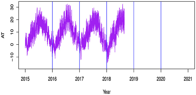
Figure 1. Shows the hourly discrete AT.

Figure 2

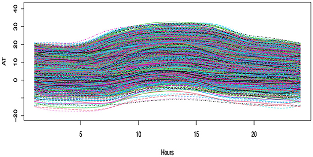
Figure 2. Illustrates the functional representation of discrete hourly air temperature data as functional curves. Each day is depicted by a single curve, resulting in a total of 2,192 curves.

Figure 3

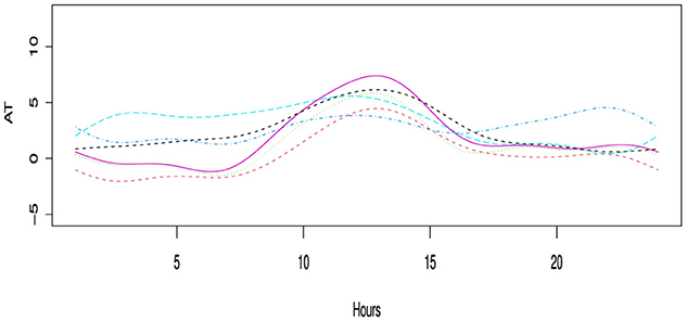
Figure 3. Represents a 1 week description of AT data into functional data.

3.2 Forecasting accuracy metrics

Two common error metrics, RMSE and MAPE, are used to assess the accuracy of the forecasting models. These error measures, which measure the degree of agreement between the actual values and the projections, are frequently employed in descriptive statistics. They are characterized in mathematics as:

$\text{RMSE}=\sqrt{\frac{1}{n}{\displaystyle \sum _{i=1}^n{\left(Y_{i,d}-{\widehat{Y}}_{i,d}\right)}^2}}$

$\text{MAPE}=\frac{1}{n}{\displaystyle \sum _{i=1}^n\left(\left|\frac{Y_{i,d}-{\widehat{Y}}_{i,d}}{Y_{i,d}}\right|\right)}\times 100$

The number of observations during the testing forecast period is denoted by n. The actual and expected AT values for the i-th day (i = 1, 2, …, 366) and the d-th hour (d = 1, 2, …, 24) are shown by - Y_{i, d} and Ŷ_{i, d}.

3.3 Results

Table 1 uses RMSE and MAPE as evaluation metrics to compare the forecasting accuracy and performance of various models. The results showed that the FAR(1) model outperformed the others due to its lowest error values. The SVM model came in second, the ANN model in third, and the NNAR model did the worst out of the four models that were assessed.

Table 1

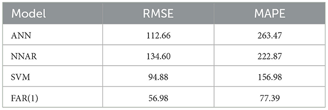
Table 1. Overall forecast results for AT.

The RMSE and MAPE measures are used to compare the hourly forecasting errors of AT from four distinct models, as indicated in Table 2. Across all hours, the FAR(1) model exhibits the highest accuracy. The SVM model outperforms the ANN model, but the NNAR model does the poorest.

Table 2

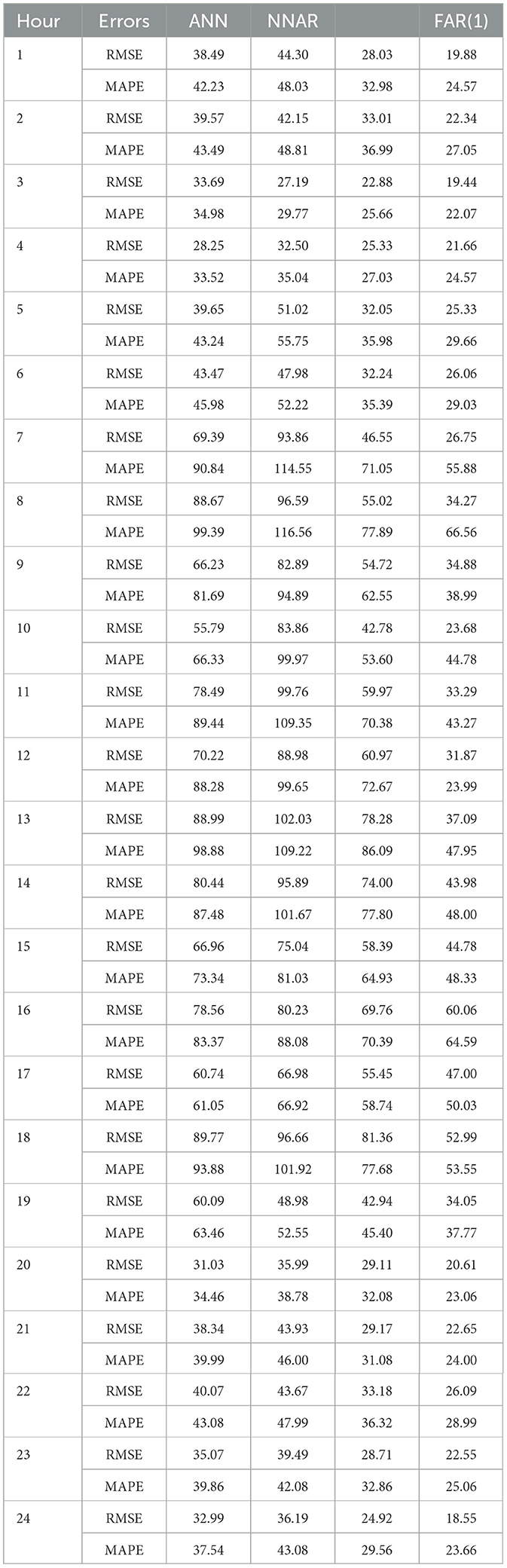
Table 2. Hour-specific forecasting errors AT.

Table 3 gives a thorough example of the RMSE and MAPE values for each month for the models that were employed to predict AT in this study. The monthly errors during the testing year are averaged to determine these errors. The findings show that forecasting mistakes differ from month to month. Notably, compared to the other months of the year, May, September, and November exhibit comparatively higher rates. Again, in nearly every month, the FAR(1) model is the best, followed by the SVM model. Again, the NNAR model is the worst across all months, and the ANN model comes in third, suggesting that it is not a good option for AT predicting.

Table 3

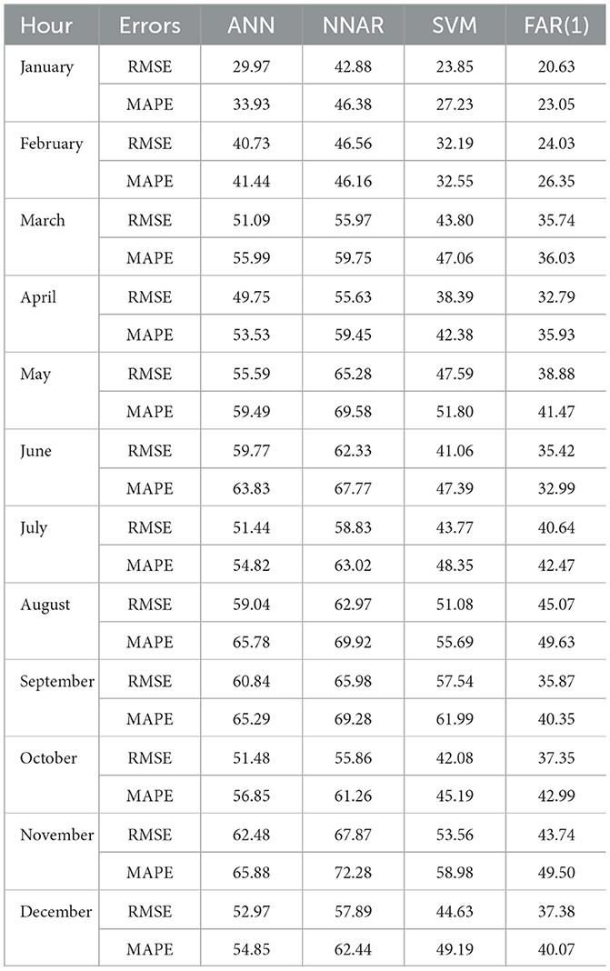
Table 3. Month-specific forecasting errors AT.

The weekly forecasting errors of the AT from four different models, measured using RMSE and MAPE as accuracy indicators, are presented in Table 4. It is observed that the proposed functional model outperforms the others, exhibiting the lowest forecasting errors across all days of the week. The SVM model ranks as the second best, followed by the ANN model in third place, while the NNAR model shows the highest forecasting errors, making it the least effective.

Table 4

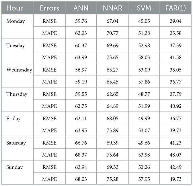
Table 4. Week-specific forecasting errors AT.

4 Conclusion

Accurate forecasting is crucial because AT is a key element of weather and affects various aspects of life. However, predicting AT is challenging due to the complex nature of ts data, which includes both random fluctuations and predictable patterns. This study introduces a method for forecasting AT one day in advance using FDA. It effectively captures AT dynamics by applying a component estimation approach that separates the data into stochastic and deterministic components. The deterministic component is modeled using smoothing splines, while the stochastic component is forecasted using FAR, SVM, ANN, and NNAR models.

For empirical analysis, AT data from Berlin, Germany, was collected. The forecasting accuracy was assessed using RMSE and MAPE metrics for one-day-ahead predictions over a full year. The results indicate that the proposed component estimation method can effectively predict AT. Compared to SVM, ANN, and NNAR models, the suggested approach significantly reduces forecasting errors and improves accuracy. Among the tested models, SVM demonstrates the lowest overall forecasting error, followed by ANN and NNAR. Additionally, ANN outperforms NNAR in terms of prediction accuracy. Overall, FAR(1) is the most effective model, followed by SVM and ANN, while NNAR performs the worst, suggesting it is not suitable for AT forecasting.

Although this study offers valuable insights, it has certain limitations. The analysis is restricted to parametric (linear) models and is based on data from a single location. Therefore, the generalizability of the FAR(1) model to other geographic regions with different climatic patterns remains an open question and should be investigated in future work. Additionally, it does not consider the impact of external variables, raising questions about how these factors might influence AT predictions in future applications of this method.

Data availability statement

The original contributions presented in the study are included in the article/supplementary material, further inquiries can be directed to the corresponding author.

Author contributions

YA: Writing – review & editing, Project administration, Resources, Supervision, Investigation. HA: Formal analysis, Investigation, Writing – original draft, Data curation. AS: Conceptualization, Data curation, Funding acquisition, Investigation, Resources, Writing – review & editing.

Funding

The author(s) declare that no financial support was received for the research and/or publication of this article.

Acknowledgments

We sincerely thank the referee for their valuable time, insightful comments, and constructive feedback, which have significantly enhanced this work. Their thoughtful suggestions have helped improve both the clarity and quality of our study. We truly appreciate their efforts in reviewing our manuscript.

Conflict of interest

The authors declare that the research was conducted in the absence of any commercial or financial relationships that could be construed as a potential conflict of interest.

Generative AI statement

The author(s) declare that no Gen AI was used in the creation of this manuscript.

Publisher's note

All claims expressed in this article are solely those of the authors and do not necessarily represent those of their affiliated organizations, or those of the publisher, the editors and the reviewers. Any product that may be evaluated in this article, or claim that may be made by its manufacturer, is not guaranteed or endorsed by the publisher.

References

1. Zahroh S, Hidayat Y, Pontoh RS, Santoso A, Sukono F, Bon A. Modeling and forecasting daily temperature in Bandung. In: Proceedings of the International Conference on Industrial Engineering and Operations Management. Riyadh (2019). p. 406–12.

Google Scholar

2. Meshram SG, Kahya E, Meshram C, Ghorbani MA, Ambade B, Mirabbasi R. Long-term temperature trend analysis associated with agriculture crops. Theor Appl Climatol. (2020) 140:1139–59. doi: 10.1007/s00704-020-03137-z

Crossref Full Text | Google Scholar

3. Hoogenboom G. Contribution of agrometeorology to the simulation of crop production and its applications. Agric Forest Meteorol. (2000) 103:137–57. doi: 10.1016/S0168-1923(00)00108-8

Crossref Full Text | Google Scholar

4. Nag P, Nag A, Sekhar P, Pandit S. Vulnerability to Heat Stress: Scenario in Western India. Ahmedabad: National Institute of Occupational Health (2009). p. 380016.

Google Scholar

5. Kumar S, Roshni T, Kahya E, Ghorbani MA. Climate change projections of rainfall and its impact on the cropland suitability for rice and wheat crops in the Sone river command, Bihar. Theor Appl Climatol. (2020) 142:433–51. doi: 10.1007/s00704-020-03319-9

Crossref Full Text | Google Scholar

6. Salman AG, Heryadi Y, Abdurahman E, Suparta W. Single layer & multi-layer long short-term memory (LSTM) model with intermediate variables for weather forecasting. Procedia Comput Sci. (2018) 135:89–98. doi: 10.1016/j.procs.2018.08.153

Crossref Full Text | Google Scholar

7. Chaudhuri S, Middey A. Adaptive neuro-fuzzy inference system to forecast peak gust speed during thunderstorms. Meteorol Atmos Phys. (2011) 114:139–49. doi: 10.1007/s00703-011-0158-4

Crossref Full Text | Google Scholar

8. Liu H, He B, Qin P, Zhang X, Guo S, Mu X. Sea level anomaly intelligent inversion model based on LSTM-RBF network. Meteorol Atmos Phys. (2021) 133:245–59. doi: 10.1007/s00703-020-00745-2

Crossref Full Text | Google Scholar

9. Li X, Li Z, Huang W, Zhou P. Performance of statistical and machine learning ensembles for daily temperature downscaling. Theor Appl Climatol. (2020) 140:571–88. doi: 10.1007/s00704-020-03098-3

Crossref Full Text | Google Scholar

10. Liu H, Mi X, Li Y. Smart deep learning based wind speed prediction model using wavelet packet decomposition, convolutional neural network and convolutional long short term memory network. Energy Convers Manag. (2018) 166:120–31. doi: 10.1016/j.enconman.2018.04.021

Crossref Full Text | Google Scholar

11. Li D, Robinson PM, Shang HL. Long-range dependent curve time series. J Am Stat Assoc. (2020) 115:957–71. doi: 10.1080/01621459.2019.1604362

Crossref Full Text | Google Scholar

12. Aue A, Norinho DD, Hörmann S. On the prediction of stationary functional time series J Am Stat Assoc. (2015) 110:378–92. doi: 10.1080/01621459.2014.909317

Crossref Full Text | Google Scholar

13. Bathia N, Yao Q, Ziegelmann F. Identifying the finite dimensionality of curve time series. Ann Statist. (2010) 38:3352–86 doi: 10.1214/10-AOS819

Crossref Full Text | Google Scholar

14. Bosq D. Linear Processes in Function Spaces: Theory and Applications, Vol. 149. Cham: Springer Science & Business Media (2000). doi: 10.1007/978-1-4612-1154-9

Crossref Full Text | Google Scholar

15. Hörmann S, Kidziński Ł, Hallin M. Dynamic functional principal components. J R Stat Soc B: Stat Methodol. (2015) 77:319–48. doi: 10.1111/rssb.12076

Crossref Full Text | Google Scholar

16. Cho H, Goude Y, Brossat X, Yao Q. Modeling and forecasting daily electricity load curves: a hybrid approach. J Am Stat Assoc. (2013) 108:7–21. doi: 10.1080/01621459.2012.722900

Crossref Full Text | Google Scholar

17. Horváth L, Kokoszka P, Rice G. Testing stationarity of functional time series. J Econ. (2014) 179:66–82. doi: 10.1016/j.jeconom.2013.11.002

Crossref Full Text | Google Scholar

18. Müller HG, Sen R, Stadtmüller U. Functional data analysis for volatility. J Econ. (2011) 165:233–45. doi: 10.1016/j.jeconom.2011.08.002

Crossref Full Text | Google Scholar

19. Zamani A, Haghbin H, Hashemi M, Hyndman RJ. Seasonal functional autoregressive models. J Time Ser Anal. (2022) 43:197–218. doi: 10.1111/jtsa.12608

Crossref Full Text | Google Scholar

20. Meintanis SG, Hušková M, Hlávka Z. Fourier-type tests of mutual independence between functional time series. J Multivar Anal. (2022) 189:104873. doi: 10.1016/j.jmva.2021.104873

Crossref Full Text | Google Scholar

21. Chang J, Chen C, Qiao X, Yao Q. An autocovariance-based learning framework for high-dimensional functional time series. J Econom. (2024) 239:105385. doi: 10.1016/j.jeconom.2023.01.007

Crossref Full Text | Google Scholar

22. Baek C, Kokoszka P, Meng X. Test of change point versus long-range dependence in functional time series. J Time Ser Anal. (2024) 45:497–512. doi: 10.1111/jtsa.12723

Crossref Full Text | Google Scholar

23. Ramsay JO. When the data are functions. Psychometrika. (1982) 47:379–96. doi: 10.1007/BF02293704

Crossref Full Text | Google Scholar

24. Ferraty F. Nonparametric Functional Data Analysis. Cham: Springer (2006).

Google Scholar

25. Ramsay J, Silverman B. Principal components analysis for functional data. In: Functional Data Analysis. Cham: Springer (2005). p. 147–72. doi: 10.1007/b98888

Crossref Full Text | Google Scholar

26. Didericksen D, Kokoszka P, Zhang X. Empirical properties of forecasts with the functional autoregressive model. Comput Stat. (2012) 27:285–98. doi: 10.1007/s00180-011-0256-2

Crossref Full Text | Google Scholar

27. Power N. Data Access Viewer. Available online at: https://power.larc.nasa.gov/data-access-viewer (Accessed 11, 2022).

Google Scholar