Modelling longitudinal cognitive test data with ceiling effects and left skewness

Cognitive tests such as the Mini Mental State Examination (MMSE) may result in data with discrete and skewed distributions that necessitate proper statistical models for valid inference. We review different longitudinal approaches to model cognitive decline data in older individuals and provide recommendations for model choice and result interpretation. We used data from the Alzheimer’s Disease Neuroimaging Initiative study and focused on MMSE scores as response variable collected on up to four visits over a two-year period in older individuals (mean age 73 years). At baseline individuals were classified as having Alzheimer’s disease (AD), early or late mild cognitive impairment, subjective memory concern, or being cognitively normal. We considered generalized additive models for location, scale and shape (GAMLSS) with binomial/beta-binomial response distribution and parametric/non-parametric random effects, selected the best model and used graphs for illustration. Binomial model with non-parametric random intercept and slope fit the data the best according to the Bayesian Information Criterion. The three-way interaction between time, age and diagnostic group was statistically significant suggesting that AD individuals had the steepest cognitive decline among all groups, especially in younger individuals. Furthermore, males and APOE4 carriers had worse cognitive performance, while more educated people had better cognitive performance compared to less educated. Various plots are used to illustrate and aid in interpretation of the results. GAMLSS are an appropriate class of models providing interpretable results for repeatedly measured cognitive test data. We recommend that they are used more widely, accompanied by effect estimation, statistical testing and visualizations for illustration.

1 Introduction

Cognitive skills like memory, problem-solving activities and speed processing deteriorate with age (1). One of the widely used cognitive tests for measuring cognitive abilities is the Mini Mental State Examination (MMSE) (2). The questions in the test are designed to assess the subject’s cognitive ability in cognitive domains such as language, orientation in time and place, memory, attention. The MMSE score is the sum of the correct answers to these questions. MMSE is an indicator of the cognitive skills of the individual and a test often used in screening for Alzheimer’s disease (AD) (3).

The Alzheimer’s Disease Neuroimaging Initiative (ADNI)¹ provides longitudinal measurements on MMSE, i.e., measurements on the same individuals over time. ADNI is “a longitudinal multicenter study designed to develop clinical, imaging, genetic, and biochemical biomarkers for the early detection and tracking of Alzheimer’s Disease (AD).” Its first goal is to “detect the disease at the earliest possible stage (pre-dementia) and identify ways to track the disease’s progression with biomarkers.”

One very distinctive feature of the MMSE score is that the cognitively normal individuals very easily obtain the maximum number of the points (30) or very close to it which creates a ceiling effect with excess observations at or close to 30 (4). Low values of the test (the minimal possible value is 0) are rarely observed. In statistical terms these two features of the data are characterized as left skewness and ceiling effect and lead to challenges in finding appropriate statistical model for such outcome as MMSE.

Standard linear mixed effects models (LMM) are often used for modelling MMSE data longitudinally. These models could be appropriately applied to such data in samples consisting mostly of people with cognitive impairment because the ceiling effect might not be present, e.g., as in Andel et al. (5). But when the study sample consists of normal individuals, for example in Jutten et al. (6) the LMM might not be appropriate due to presence of ceiling effect in the data.

Transformations are sometimes used to normalize the data, e.g., Jacqmin-Gadda et al. (7) applied transformations but this approach might not always solve the problem with the ceiling effect because the equal values in the original scale remain equal in the transformed scale. If there is a relatively large percentage of healthy individuals in a sample, the resulting distribution would still have a pronounced ceiling effect and would fail the assumption of normal distribution even after transformation.

Models for discrete data such as the binomial or beta-binomial model are expected to fit better than the standard linear model because they can handle both features of such data: skewness and ceiling effects. Recall that the MMSE score is a sum of the correct answers to multiple questions. If the questions could be considered independent with the same probability of a correct answer, then the total MMSE score would follow a binomial distribution. However, the independence assumption does not necessarily hold since the correctness of individual’s answer to one question might be related to the correctness of their answer to another question resulting in increased between-subject variability. When there is more variability in the data that cannot be captured by the binomial model, a more appropriate model could be the beta-binomial. The latter model suggests that the binomial parameter is a random variable itself that follows beta distribution. This model has more parameters that allow more flexibility in modelling the variance of the outcome. In our work we consider binomial and beta-binomial models for longitudinal data, but both models are used for cross-sectional MMSE data as well.

In longitudinal data scenarios, we also need additional modifications of the models compared to cross-sectional data. One of the main characteristics of longitudinal data is the correlation between repeated observations on the same subject. In contrast to the possible correlation of questions within individual, herein we refer to the correlation between MMSE scores collected on the same individual over time. Mixed effects models (8), take into account this within-subject correlation of the data via random effects which take the same value within individual and potentially different values for different individuals. These additional terms in the model are typically assumed to have a parametric distribution (e.g., normal). They are introduced to capture between-individual variability regarding different starting points and different slopes over time with random intercept and random slope terms, respectively, that vary continually within the population of individuals. The well-known class of models with parametric random effects but with a variety of distributions for the outcome including binomial is called Generalized Linear Mixed Models (GLMM) (9) and they generalize LMM for normal data.

Another option for the distribution of the random effects in longitudinal data is to consider them non-parametric, i.e., to assume that random effects take a number of possible values (also called mass points) with particular probabilities for each. The number of mass points is not known in advance and it has to be determined from the data relying on some criterion, for example Akaike Information Criterion (AIC) (10) and/or Bayesian Information Criterion (BIC) (11). We want to note that both criteria (AIC and BIC) are used for model selection in a much broader context, not only for selecting the number of mass points.

Both binomial and beta-binomial models with non-parametric random effects are special cases of the generalized additive models for location, scale and shape (GAMLSS) (12). Here we present those two models with parametric/non-parametric random effects. We believe that from a theoretical perspective this is the most appropriate approach for longitudinal discrete data such as the MMSE which is characterized with left-skewness and ceiling effects. We use the models to estimate the effects of level of cognitive impairment and age on cognitive functioning over time, while controlling for gender, years of education, marital status, number of copies of allele 4 of the APOE gene in the ADNI data. We focus on model selection, parameter estimation and assessment of model fit. We emphasize interpretability and provide several visual and analytical aids for understanding the results.

2 Materials and methods

2.1 Participants

Our study sample in the motivating data consists of 1945 individuals that form five groups according to their diagnosis at baseline: Alzheimer’s disease (AD, n = 342); late mild cognitive impairment (LMCI, n = 596); early mild cognitive impairment (EMCI, n = 332); significant memory concern (SMC, n = 211) and cognitively normal (CN, n = 464). Each individual belongs in only one of the five groups. The individuals grouping criteria are available in the ADNI protocols available at: https://adni.loni.usc.edu/wp-content/themes/freshnews-dev-v2/documents/clinical/ADNI-2_Protocol.pdf, page 18. The distinction between the different groups is based on different measures of the cognitive abilities of the individuals and other factors as stability of permitted medications for 4 weeks. We included individuals with at least two out of four longitudinal measurements that we considered – at baseline, 6, 12 and 24 months after the baseline measurement. According to the ADNI protocol² the study was conducted according to Good Clinical Practice guidelines, the Declaration of Helsinki, US 21CFR Part 50 – Protection of Human Subjects, and Part 56 – Institutional Review Boards, and pursuant to state and federal HIPAA regulations.

2.2 Measures

2.2.1 Outcome variable

The variable of main interest is the total MMSE score. As mentioned before, the MMSE test consists of 30 questions. Each correct answer brings one point to the final score. The MMSE score is the number of correct answers, and it is an integer between 0 and 30. Higher values of the MMSE score indicate better cognitive function. We consider the measurements at baseline, 6 months, 12 months and 24 months after the baseline measurement. According to the ADNI protocols all individuals should be examined through this cognitive test at these time points. However, like almost any longitudinal study, there is missing data. In our analysis we use all available data on individuals with at least two observations out of the four.

Descriptive statistics of the MMSE (mean and standard deviation) for the five diagnosis groups over time are presented in Table 1. We notice some deterioration in cognitive performance for some groups of individuals – most notable for the AD and LMCI groups. For the EMCI group there is little change. The SMC and CN groups stay at the same levels at the four time points and are almost identical.

Table 1

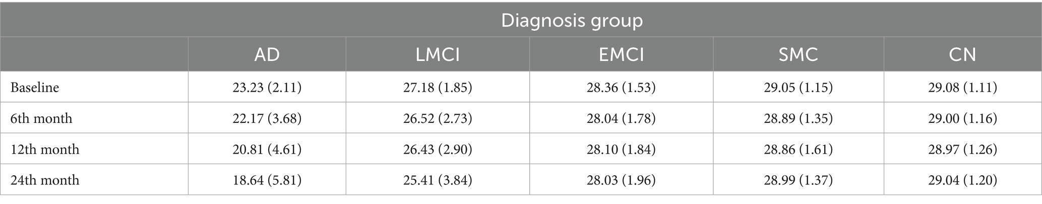
Table 1. Mean (standard deviation) of Mini Mental State Examination for the five groups of individuals at the four time points—baseline, 6 months, 12 months, and 24 months.

In Figure 1 we present boxplots of the MMSE observations at the different time points grouped according to diagnosis at baseline. At the bottom of each boxplot, we give the number of the observations at the corresponding time point. We clearly notice a worsening of the performance on the test over time for most people, especially in the AD group. The LMCI group has the same trend although not at the same rate as the AD group while the CN group has almost no change in MMSE performance over time.

Figure 1

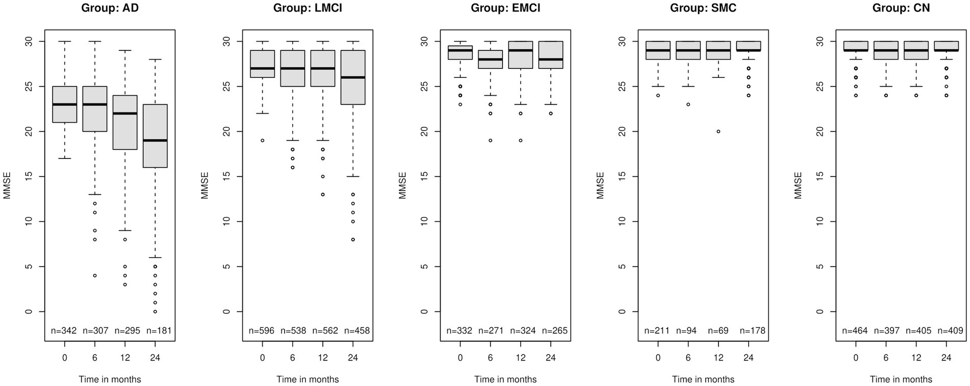
Figure 1. Boxplots of the Mini Mental State Examination (MMSE) for the five group of individuals according to the diagnosis at baseline: AD, Alzheimer’s disease; LMCI, late mild cognitive impairment; EMCI, early mild cognitive impairment; SMC, significant memory concern; CN, cognitively normal at the four different time points – baseline, 6 months, 12 months and 2 years after the baseline measurement. At the bottom “n” is the number of observations at the corresponding time point.

2.2.2 Predictor variables

The main predictors are time (treated as continuous variable), diagnosis at baseline, age at baseline, gender, number of the copies of allele 4 of gene APOE, years of education, marital status.

Descriptive statistics of the predictor variables at baseline according to diagnosis group are presented in Table 2. We notice that the mean age of the EMCI and SMC individuals is smaller than the mean age of the other three groups. CN subjects have one more year of education on average compared to the AD subjects. The biggest percentage of people with two copies of allele 4 of the APOE gene is in the AD group.

Table 2

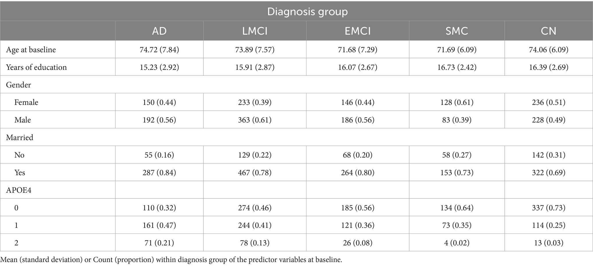
Table 2. Descriptive statistics of the predictors within diagnosis group.

2.3 Statistical models

We modelled the MMSE score longitudinally from the data available at the four time points (baseline, 6 months, 1 year and 2 years after the baseline measurement) through main effects of all the predictor variables, described in the previous section, all two-way interactions between time, diagnosis and age at baseline and the three-way interaction between time, diagnosis, and age at baseline. For easier interpretation of the results, we centered baseline age in the analyses by subtracting the mean age (73 years) from the age of each individual. The variable APOE4 is considered with additive allele effect.

We fit binomial and beta-binomial generalized additive models for location, scale and shape (GAMLSS) models (13) to the data. GAMLSS extend the basic Generalized Linear Model (GLM) (14) in several ways. The basic GLMs describe the mean of the dependent variable given the predictors: $\mathrm{E}(\mathrm{Y}\mid \mathrm{X})={\mathrm{g}}^{-1}\left(\mathit{X\beta }\right)$ , where $\mathrm{E}(\mathrm{Y}\mid \mathrm{X})$ is the expected value of $\mathrm{Y}$ conditional on the predictors $\mathrm{X}$ , $\mathit{X\beta }$ is the linear predictor, a linear combination of unknown parameters β and $g$is the link function. The distribution of the outcome variable $\mathrm{Y}$ belongs to the GLM if its density or probability function defines a distribution in the exponential family (e.g., normal, binomial, Poisson). Additionally to modelling the mean of the dependent variable in the GLM framework, GAMLSS models allow three other parameters of the distribution to be modelled via the explanatory variables – scale parameter related to the variance of the distribution and two shape parameters which are often related to the skewness and kurtosis of the distribution. GAMLSS models also allow linear or nonlinear parametric functions, or nonparametric smoothing functions of explanatory variables (13). GAMLSS models include a very broad class of distributions (e.g., beta-binomial) in addition to the ones in GLM thus allowing for more unusual data (e.g., with floor/ceiling effects, skewness). They also include random effects with parametric or non-parametric distributions thus allowing for great flexibility in capturing between-subject heterogeneity in means and/or variances and correlations among repeated observations on the same individual. Applications of GAMLSS models could be found in Muniz-Terrera et al. (14) where beta-binomial distribution is used and in Brati (15) where lognormal distribution is used. More examples of applications of GAMLSS could be found in Von Heimburg et al. (16) and Tu et al. (17).

To model change in MMSE over time, due to the longitudinal character of the data, we included random effects in the models to account for the correlation between the observations on the same subject. We considered both parametric and non-parametric distribution for the random effects. In the parametric case, we considered random intercept binomial model with normal distribution of the random term. Then we considered random intercept model, and random intercept and slope models for binomial and beta-binomial distribution with 1–10 mass points for the non-parametric random effects. We decided on the best model depending on the BIC values of the models. The GAMLSS models that we considered in this work are implemented in R in two packages: the gamlss package³ (12) and the gamlss.mx package.⁴ We implemented R code for the calculation of the randomized quantile residuals (18), to explore if the model assumptions are satisfied.

3 Results

The results for the BIC for the different models fitted to the data are presented in Table 3. The models with the smallest values of BIC within each model are in red. Comparing among all models, we observe that the best model fit is binomial random intercept and slope model with 6 mass points.

Table 3

Table 3. Model comparison based on the Bayesian information criterion (BIC).

The following Equation 1 describes the model:

$\begin{array}{l}\text{logit}\left(p_{\mathit{ij}}\right)=b_{i0}+b_{i1}{\text{Time}}_{\mathit{ij}}+{\beta }_0+{\beta }_1{\text{Time}}_{\mathit{ij}}+{\beta }_2\mathrm{I}({}_{\mathrm{CN})}\\ +{\beta }_3\mathrm{I}({}_{\text{EMCI})}+{\beta }_4\mathrm{I}({}_{\text{LMCI})}+{\beta }_5\mathrm{I}({}_{\mathrm{SMC})}+{\beta }_6{\mathrm{Age}}_{\mathit{ij}}\\ +{\beta }_7{\text{YearsEduc}}_{\mathit{ij}}+{\beta }_8{\mathrm{APOE4}}_{\mathit{ij}}+{\beta }_9\mathrm{I}{\left(\text{Male}\right)}_{\mathit{ij}}\\ +{\beta }_{10}\mathrm{I}{\left(\text{Married}\right)}_{\mathit{ij}}+{\beta }_{11}\mathrm{I}({{}_{\mathrm{CN})}}^{\ast }{\text{Time}}_{\mathit{ij}}\\ +{\beta }_{12}\mathrm{I}({{}_{\text{EMCI})}}^{\ast }{\text{Time}}_{\mathit{ij}}+{\beta }_{13}\mathrm{I}({{}_{\text{LMCI})}}^{\ast }{\text{Time}}_{\mathit{ij}}\\ +{\beta }_{14}\mathrm{I}({{}_{\mathrm{SMC})}}^{\ast }{\text{Time}}_{\mathit{ij}}+{\beta }_{15}{{\mathrm{Age}}_{\mathit{ij}}}^{\ast }{\text{Time}}_{\mathit{ij}}\\ +{\beta }_{21}\mathrm{I}({{}_{\mathrm{CN})}}^{\ast }{\mathrm{Age}}_{\mathit{ij}}+{\beta }_{22}\mathrm{I}({{}_{\text{EMCI})}}^{\ast }{\mathrm{Age}}_{\mathit{ij}}\\ +{\beta }_{23}\mathrm{I}({{}_{\text{LMCI})}}^{\ast }{\mathrm{Age}}_{\mathit{ij}}+{\beta }_{24}\mathrm{I}({{}_{\mathrm{SMC})}}^{\ast }{\mathrm{Age}}_{\mathit{ij}}\\ +{\beta }_{111}\mathrm{I}({{}_{\mathrm{CN})}}^{\ast }{{\text{Time}}_{\mathit{ij}}}^{\ast }{\mathrm{Age}}_{\mathit{ij}}+{\beta }_{112}\mathrm{I}({}_{\text{EMCI})}\\ {}^{\ast }{{\text{Time}}_{\mathit{ij}}}^{\ast }{\mathrm{Age}}_{\mathit{ij}}+{\beta }_{113}\mathrm{I}({{}_{\text{LMCI})}}^{\ast }{{\text{Time}}_{\mathit{ij}}}^{\ast }{\mathrm{Age}}_{\mathit{ij}}\\ +{\beta }_{114}\mathrm{I}({}_{\mathrm{SMC})}\ast {{\text{Time}}_{\mathit{ij}}}^{\ast }{\mathrm{Age}}_{\mathit{ij}}\\ j=1,2,3,4;i=1,\dots ,1945,\end{array}\text{ (1)}$

where the index $i$ is for the individual, the index $j$ is for the time point - baseline, 6 months, 12 months and 2 years after the baseline measurement and $p_{\mathit{ij}}$ is the probability the individual $i$ to give a correct answer at time point $j$ . In the original notation, the parameter on the left-hand side of the above equation is denoted by $\mu$ . However, we denote the parameter by $p$ to emphasize the fact that it comes from Bernoulli trials. In our case we consider the distribution of the MMSE score to be binomial distribution with parameters Bi(30, p). The random effects for each individual $(b_{i0},b_{i1})$ are among the 6 possible mass points.

Indicator variables $\mathrm{I}$ (∗) for diagnosis at baseline are

• $\mathrm{CN}$ - cognitively normal;

• $\text{EMCI}$ - early mild cognitive impairment;

• $\text{LMCI}$ - late mild cognitive impairment;

• $\mathrm{SMC}$ - significant memory concern;

• $\mathrm{AD}$ - Alzheimer’s disease, reference level.

The best-fitting model estimates are shown in Table 4.

Table 4

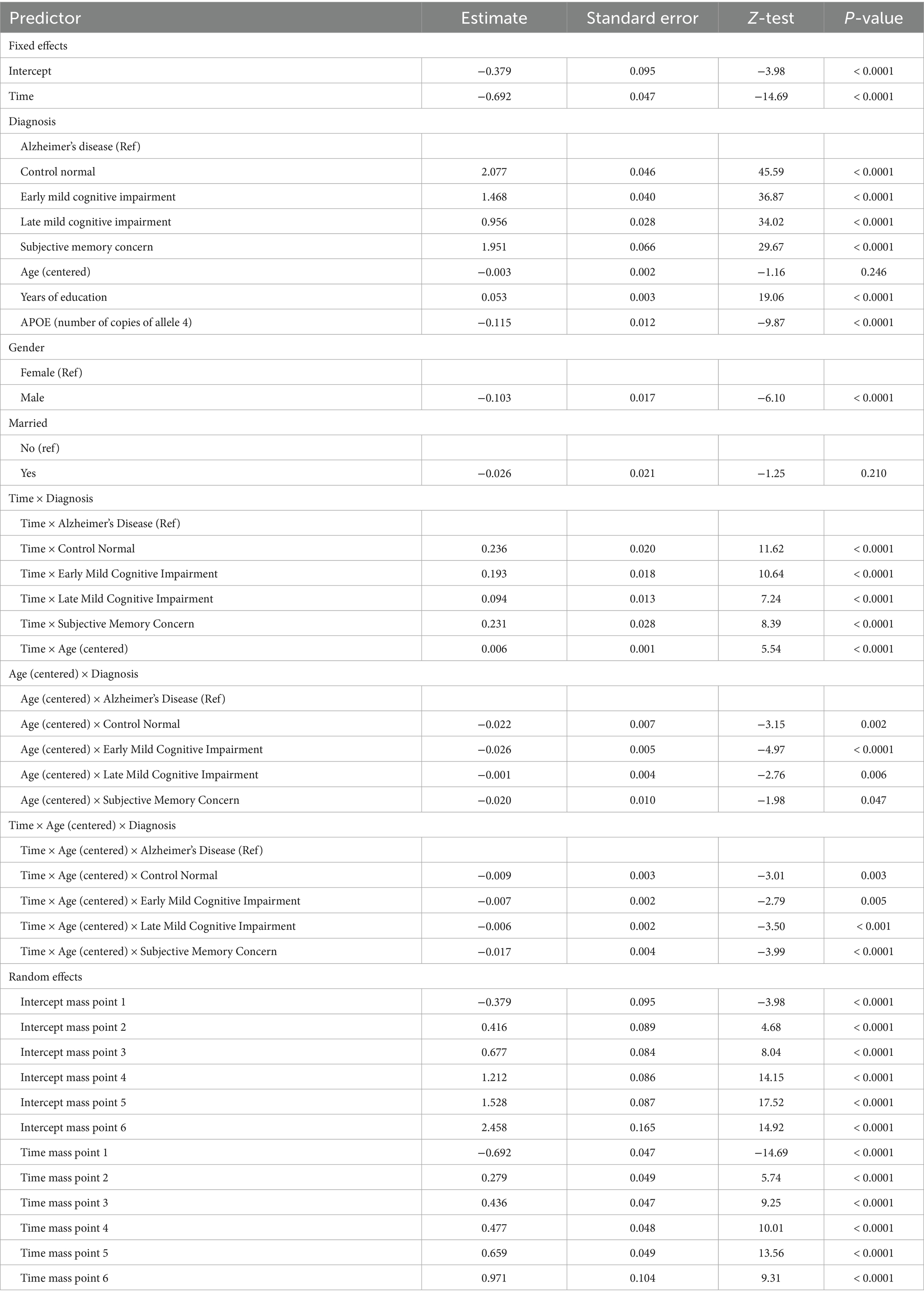
Table 4. Estimates, standard errors, test statistics, and p-values for the fixed and random effects in the final binomial model with six mass points for the random effects.

The three-way interaction between time, age at baseline and diagnosis is statistically significant. There are also significant two-way interactions between time and age, age and diagnosis, and time and diagnosis. Males and people with copies of allele 4 have worse cognitive functioning while more educated people have better cognitive functioning.

The random effects are also presented in Table 4 in a section of the table after the fixed effects. For the mass points from the second to the sixth, the coefficients presented in Table 4 are the differences between the respective mass point and the first mass point. The first mass point is directly presented in the table. The calculations of the values of the rest of the mass points is also explained in Muniz-Terrera et al. (14). These calculations are valid both for random intercept and the random slope, i.e., the second mass point has values (−0.379 + 0.416) = 0.037 for the random intercept and (−0.692 + 0.279) = −0.413 for the random slope. The values of the rest of the mass points can be calculated similarly.

The estimated distribution of the random effects shows that the third, fourth and fifth random effects account for 88% of random effects across all subjects (34% for the third, 27% for the fourth and 26% for the fifth). Then the second random effect accounts for almost 8%, the sixth - for 4% and the first – for <1%.

Several figures aim to better illustrate the results. In particular, Figure 2 shows the predicted values of MMSE for the five groups of individuals at the most probable random effects (the third mass point), at three different ages at baseline (mean age of 73, 66 years and 80 years which are the mean age minus/plus one standard deviation of the age), for females who are not married, have no copies of allele 4 of the APOE gene and have 16 years of education (i.e., at the mean years of education). We notice the different speed of decline of the diagnosis groups which is due to the statistically significant interaction between age, diagnosis group and time. People who are diagnosed with AD earlier in life have a much steeper decline than people who are diagnosed at the mean age of the sample and even at age that is one standard deviation above the mean age of the sample subjects, i.e., 73 and 80 years. Another observation is that people with subjective memory concern are very similar to cognitively normal people. We see some difference between these two groups only for the oldest subgroup. We also notice that the LMCI group has relatively steep negative slope. The interaction effect between age and time is most pronounced for the AD group.

Figure 2

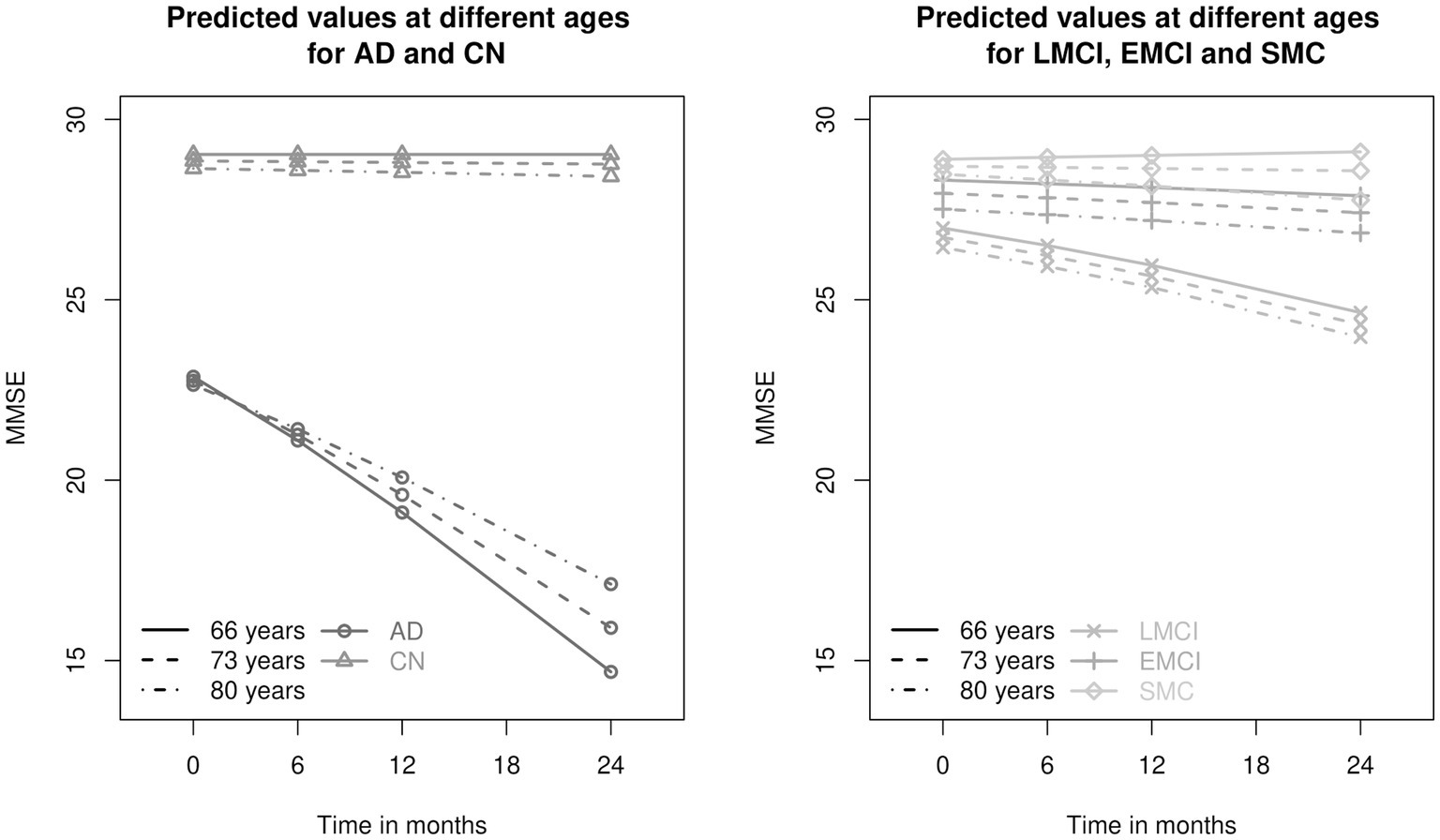
Figure 2. Predicted values of Mini Mental State Examination (MMSE) for the five different diagnosis groups: AD, Alzheimer’s disease; LMCI, late mild cognitive impairment; EMCI, early mild cognitive impairment; SMC, significant memory concern; CN, cognitively normal at three different ages - 66, 73 and 80 years. The ages are the mean age and the mean age plus/minus one standard deviation (the mean age at baseline is 73 years and the standard deviation is 7 years). The AD and CN groups are presented on the left panel, the LMCI, EMCI and SMC groups - on the right-hand side.

We illustrate the discrete structure of the six random effects in Figure 3. We compare the trajectories of married EMCI and LMCI females with a side-by-side plot. Again, we focus on 73 years old females who are not married, who have no copies of allele 4 of the APOE gene and who have 16 years of education, although the predicted lines for other types of individuals at mean age will be parallel to the corresponding lines shown in Figure 3. The thickness of the lines corresponds to the estimated probability of the random effects (the thicker the line the more probable the random effect is). The trajectories are very similar with one exception – EMCI individuals with the third or fourth random effects show almost no change over time while LMCI individuals with the same random effects show decline over time. This is due to the statistically significant interaction between time and diagnosis.

Figure 3

Figure 3. Predicted values of Mini Mental State Examination (MMSE) for early mild cognitive impairment (EMCI) are presented on the left-hand side and late mild cognitive impairment (LMCI) – on right-hand side for different random effects. The thickness of the line of each random effect corresponds to the probability of the random effect (RE)- the thicker the line the more probable the random effect is.

We performed statistical tests to compare all pairs of diagnosis groups at three different ages (mean age and one standard deviation above and below the mean age). These comparisons were performed at baseline, at two-year follow-up, and for the change from baseline to two years. Because there are 90 tests, we performed Benjamini-Hochberg correction for multiple comparisons (19). The results from the statistical tests are presented in Figure 4. They show that the AD group is different from the other groups in all considered settings. No statistically significant differences between the cognitively normal and the SMC groups were found in the data.

Figure 4

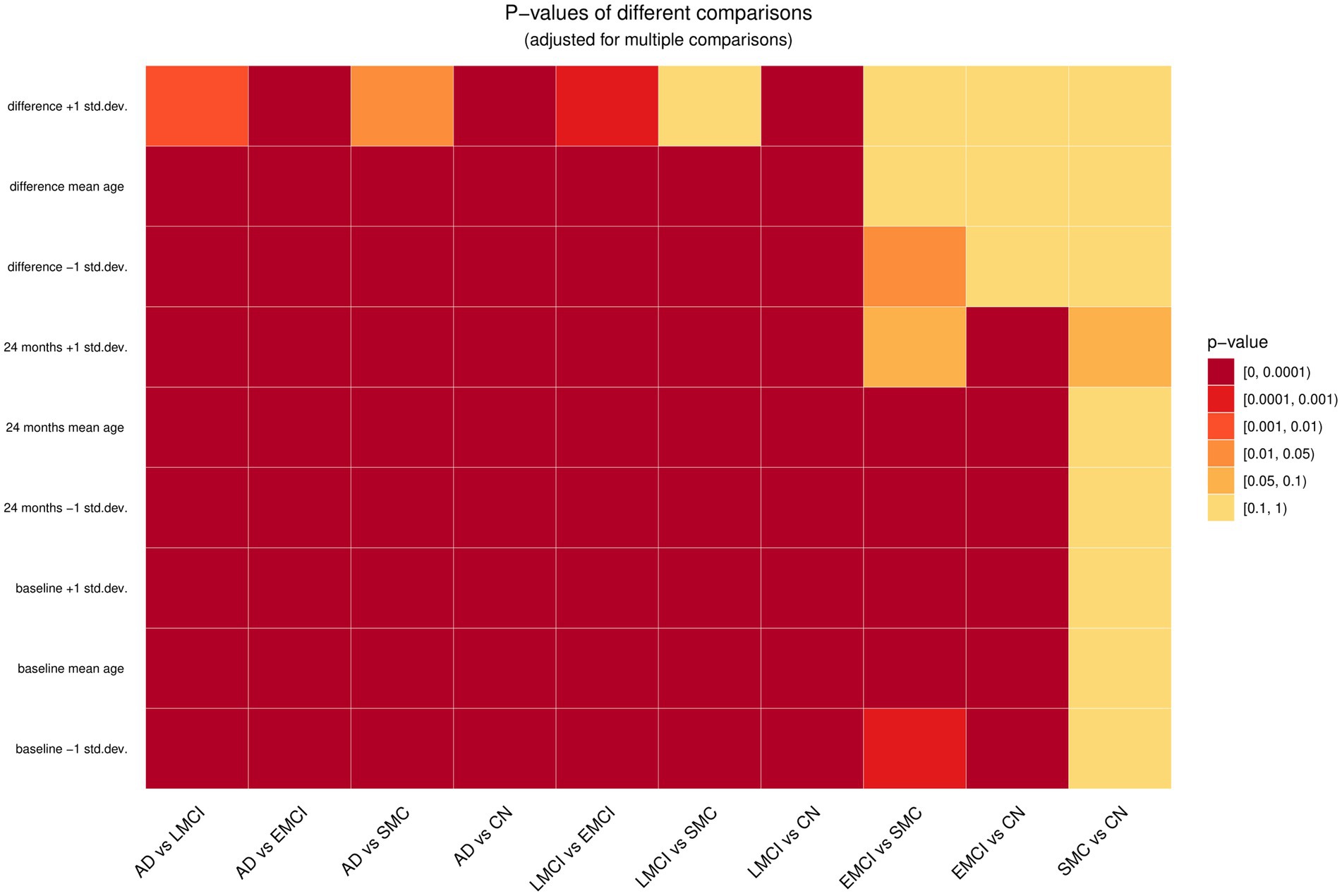
Figure 4. Comparison of all pairs of diagnosis groups at baseline, last time point and the difference of these two time points at three ages – mean age and plus/minus one standard deviation from the mean age (66, 73, and 80 years). The five different diagnosis groups are: AD, Alzheimer’s disease; LMCI, late mild cognitive impairment; EMCI, early mild cognitive impairment; SMC, significant memory concern; CN, cognitively normal.

To perform the tests described above we needed the covariance matrix of the estimates which was not provided by the build-in R function that fitted the model. For this reason, we applied a bootstrap method to estimate the covariance matrix. The algorithm implemented is the following:

1. Random draw for the random effect for each individual using the estimated probability distribution.

2. Binomial draw according to the fitted probability from the model calculated using the predictors of the observed data and the sampled random effect in Step (1).

3. Estimation of the model coefficients given the data generated for the outcome in Step (2) and the observed predictors.

4. Repetition of Step (1) to Step (3) 1,000 times.

5. Calculation of the covariance matrix of the estimated coefficients.

We used randomized quantile residuals to examine if the assumptions of the model are met. Figure 5 shows a Q-Q plot (left-hand side) and a plot of the residuals versus the fitted values (right-hand side). We notice that some residuals are smaller than expected (visible on the left-hand side of the Q-Q plot). We identified the individual observations they correspond to and noticed that these residuals are for individuals for which we observe unexpected steep decline in the score of MMSE that cannot be captured by the model.

Figure 5

Figure 5. Q-Q plot of the randomized quantile residuals of the model are presented on the left-hand side. Residuals versus fitted values are presented on the right-hand side of the plot.

4 Discussion

The aim of our work was to identify and recommend an appropriate longitudinal model for cognitive performance data that exhibit both ceiling effects and left skewness. We were motivated by the MMSE data of individuals with different levels of cognitive difficulties from the ADNI studies over a two-year period and used these data to demonstrate our approach. We considered the effects of diagnosis at baseline, age at baseline, time, all possible interactions of these predictors, the number of copies of allele 4 of gene APOE, marital status, gender, and the years of education.

From literature review we identified the GAMLSS class of models as the most appropriate class of models but there were several choices of possible distributions for the outcome from that class. Since MMSE data are discrete and show characteristics of ceiling effect and left skewness, the binomial and beta-binomial models provide suitable options to capture the nature of the response distribution and they guarantee that the fitted and predicted scores are in the range of the original scale. They also accommodate both ceiling effects and negative skewness. The beta-binomial model compared to the binomial model allows to accommodate bigger population variance which to some degree may take into account the effect of the correlations of the answers within one MMSE test. Both models are easy to fit with the R packages gamlss and gamlss.mx and provide interpretable results that are illustrated in this data example. We believe that substantial improvement could be made to applications in medical discrete data with ceiling and/or floor effect by using the GAMLSS class of models instead of LMM. The normal distribution (assumed in LMM) is likely to produce fitted values outside the range of the MMSE due to the ceiling effect and introduces a dependence between residuals and fitted values which is a violation of the model assumptions (14). The GAMLSS approach includes many distributions under its umbrella and can provide a better fit to MMSE type data.

Since MMSE testing in ADNI is repeated over time, with GAMLSS we can also capture the rate of decline in cognitive performance while taking into account the features of the data described in the previous section. Random effects are necessary to capture the correlation between repeated MMSE measurements on the same individual over time. The random effects could be parametric (usually assumed to be normally distributed) or non-parametric. Most often researchers make assumptions that the effects are parametric, however for MMSE data that are discrete, non-parametric framework is more appropriate. More detailed and technical discussion about the advantages of the non-parametric approach is provided in Muniz-Terrera et al. (14). In this application we considered both parametric and non-parametric random effects and the statistical criteria indicated that models with non-parametric effects fit better. We note that between the two statistical criteria used most often to find a best-fitting model among candidate models (i.e., AIC and BIC) we selected the BIC because it emphasizes model parsimony. We compared binomial and beta-binomial models using BIC which on its own may not fully capture overdispersion, especially when random effects are present. As a result, we assessed the potential overdispersion in an indirect manner. Formal residual diagnostics or overdispersion tests could be useful aspects for exploration in future research.

The idea of models with finite number of mass points, i.e., non-parametric random effects, is similar to latent class growth analysis (LCGA) (20). The latter is a class of models that assumes that individuals are grouped into latent classes with the same trajectories over time within class. In this respect, binomial and beta-binomial non-parametric random effects models are similar to latent class growth analysis for discrete data because the individuals who have the same random terms, i.e., random effects (among a finite number of possible options), belong to the same latent class and have the same pattern over time. Having a fixed number of random effects (in our case 6) implies that we have the same number of basic trajectories for the population of individuals over time. These trajectories can be further varied due to the values of the additional fixed covariates in our model. Thus, we have both flexibility and parsimony in modeling patterns of change over time. It is important to note that our framework does not estimate individual group membership. While the random effects distribution is modeled nonparametrically to flexibly capture individual variability, our approach differs from traditional latent class models, which assign individuals to specific latent classes.

The basic trajectories could be regarded as latent subgroups as encountered in latent class growth modeling. However, rather than modeling the effect of covariates on subgroup membership as is typically done in latent class models, we model the effects of covariates directly on the outcome. Since we have only 4 time points, we focus on linear trends over time although our approach could be extended to higher order terms (e.g., quadratic). Typically, latent glass growth modeling considers standard response distributions (e.g., normal, Poisson) whereas the GLAMSS provide more flexibility in modeling data with non-standard distributions. For the data set that we considered the model with binomial distribution and six non-parametric random effects fit the data the best. Our model identified a significant three-way interaction between age at baseline, time and diagnostic group thus indicating that cognitive deterioration proceeds at different speeds depending on diagnosis at baseline and age. Especially worrisome is the steep decline in the AD group, most pronounced for individuals who are younger at baseline. This is consistent with the literature on the severity and the poor prognosis of early-diagnosed Alzheimer measured as rate of change in MMSE (21). More recent article claims that trajectory of a single outcome fails to capture disease progression comprehensively and there is substantial heterogeneity in the AD progression (22).

Possession of at least one copy of allele 4 of apolipoprotein E (APOE) is known to be the strongest risk factor for developing sporadic form of AD (23). It is known that it is associated with an increase in the levels of amyloid deposition and an early age of onset of AD (24). Emrani et al. (23) identifies AD patients carriers of allele 4 APOE as patients with more amnestic cognitive profile than the non-carriers AD patients. Gharbi-Meliani et al. (25) finds that individuals with 2 copies of allele 4 of APOE have poorer global cognitive score starting from 65 years. We found that individuals who are carriers of one copy of allele 4 of the gene APOE 4 have worse cognitive performance on the MMSE compared to non-carriers. Also, the model assumes that the effect is double for carriers of two copies of this allele and this is the same across all diagnosis groups of individuals. Note that in this example we did not consider whether there are interactions involving the APOE gene with other predictors in the model. This is because we were focused on demonstrating the process of identifying a well-fitting model but exploring interactions of other factors is certainly a possible avenue for further research.

Our emphasis was also on illustrating how the model results, including interactions between baseline factors and time, can be better interpreted via additional tests and figures. Figures of predicted responses over time at different levels of the model variables using features such as thickness of the lines illustrating the likelihood of observing a particular trajectory are helpful in conveying results to a wider audience. Using heat maps to simultaneously present the significance of multiple comparisons is also a handy way to present important points. Finally, we suggest that researchers always examine residual plots as they give indication whether the model fits the data well and for what kind of observations or outliers it may not provide a good fit.

MMSE is a cognitive test widely used for screening of AD. Still, for example there are no strict thresholds for the classification of cognitively normal individuals depending on the MMSE score. A main result of a systematic review (26) on the subject is about the specificity and sensitivity of two widely used cutoff points - 24 and 25. For example in ADNI the normal subjects are those with MMSE score equal to or greater than 24. In Muniz-Terrera et al. (14) the cognitively normal individuals are in the range 25–30 whereas individuals with scores between 24 and 10 are said to be cognitive impaired, whilst scores below 10 are indicative for dementia. Our model allows for prediction of future responses and this way may be used to predict when individuals cross a certain threshold and are expected to move in another cognitive group. We want to point out that the diagnosis of AD is very complex and may require blood tests, MRI, CT or PET brain imaging. Thus, MMSE is only indicative about the cognitive skills of the individual. The predictions provided by our model in addition to other clinical data could be used to inform intervention strategies.

A limitation of the R function when applied to our data was that the function that fitted the model did not provide the covariance matrix of the estimates. In cases in which we need the covariance matrix of the estimates we propose a bootstrap method for its estimation. Such cases are for example in situations in which we want to compare some groups of individuals and the hypothesis test involves more than one parameter of the model.

In our work we did our analyses on the available data without exploring in detail the missing data mechanism. The chi-squared test for comparing the proportion of dropout at the last time point among the five diagnosis groups was statistically significant (p-value < 0.0001). If anything, our results are more conservative because the dropout in the AD group is higher and the differences between the groups would be even greater. But also, due to the AD group’s higher dropout rate, there is a possibility that dropout is linked to unobserved cognitive decline. If the missingness is indeed associated with unmeasured deterioration, bias from a Missing Not at Random (MNAR) mechanism could arise. Given that we have random effects in the model and use maximum likelihood estimation, our approach produces unbiased and efficient estimates when the missing data mechanism is Missing at Random (MAR) (27). However, if the mechanism is MNAR then we might expect some bias in the estimation, however we cannot distinguish MAR and MNAR mechanisms from the observed data (28). There is vast literature on the different approaches to cope with missing data and under what assumptions the conclusions from the analysis on the available data are valid (28). Future direction of research is to apply statistical methods designed for coping with missing data.

The model is limited by our goal to be able to make predictions about future cognitive functioning as early as possible and therefore use only information on the diagnosis at baseline. Modelling the change of diagnosis over time and maybe its effect on functioning will be a different problem and may require a different statistical model (e.g., Markov model). Additionally, some individuals initially classified as having MCI may later revert to normal cognitive status or fail to consistently meet the criteria for impairment. This limitation, inherent to the ADNI study design, may affect how baseline group comparisons are interpreted. It is worth noting the potential for misclassification when using a single time-point MCI diagnosis. Diagnostics for influential observations were not performed in this analysis. MMSE scores are bounded and susceptible to ceiling and floor effects and a few extreme observations could significantly influence the results, hence identifying influential observations is an important topic for future research.

Our work was motivated by repeatedly measured cognitive test data. The discreteness, skewness and ceiling effect of the data require the use of an appropriate model. We found that the GAMLSS class of models are well-suited to the data, very flexible and easy to fit with freely available software. To aid in interpretation of results we supplemented statistical testing and estimation with graphical illustrations. In conclusion, we recommend that GAMLSS models are used more widely for this type of data and interpreted with the aid of statistical estimates and visualizations. This paper is one of the few studies to use GAMLSS with non-parametric random effects for longitudinal cognitive data, demonstrating that this approach offers advantages compared to conventional linear mixed models.

5 Conclusion

The aim of our research was to find an appropriate longitudinal model for modeling cognitive function data on individuals with different cognitive abilities at baseline and to provide visualization methods to complement statistical testing and inference. In the motivating data, we found that AD individuals had the steepest cognitive decline among all groups, especially in younger individuals. Furthermore, males and APOE4 carriers had worse cognitive performance, while more educated people had better cognitive performance compared to less educated. The importance of this work is that with GAMLSS models we both respect the nature of the data (discrete left-skewed with ceiling effect) and are able to interpret and illustrate the findings from a sophisticated statistical model to practitioners in the field.

Data availability statement

The data analyzed in this study is subject to the following licenses/restrictions: the data used to support the findings of this study are available from ADNI upon application approval. Requests to access these datasets should be directed to ADNI. Data used in preparation of this article were obtained from the Alzheimer’s Disease Neuroimaging Initiative (ADNI) database (adni.loni.ucla.edu). As such, the investigators within the ADNI contributed to the design and implementation of ADNI and/or provided data but did not participate in analysis or writing of this report. A complete listing of ADNI investigators can be found at: https://adni.loni.usc.edu/wp-content/uploads/how_to_apply/ADNI_Acknowledgement_List.pdf.

Ethics statement

Ethical approval was not required for the study involving humans in accordance with the local legislation and institutional requirements. Written informed consent to participate in this study was not required from the participants or the participants’ legal guardians/next of kin in accordance with the national legislation and the institutional requirements.

Author contributions

DG: Conceptualization, Software, Visualization, Writing – original draft, Formal analysis, Methodology, Data curation, Writing – review & editing. DP: Supervision, Conceptualization, Writing – review & editing. RG: Writing – review & editing, Supervision, Conceptualization, Methodology.

Funding

The author(s) declare that financial support was received for the research and/or publication of this article. DG was supported by the GATE project. The project has received funding from the European Union’s Horizon 2020 WIDESPREAD-2018-2020 TEAMING Phase 2 programme (Grant agreement no. 857155). DP was supported by the European Union -NextGenerationEU, through the National Recovery and Resilience Plan of the Republic of Bulgaria, project no. BG-RRP-2.004-0008.

Acknowledgments

Some computations were performed on the supercomputer Avitohol described in Atanassov et al. (29). The authors acknowledge the provided access to the infrastructure purchased under the National Roadmap for RI, financially coordinated by the MES of the Republic of Bulgaria (grant no. D01-325/01.12.2023). Data collection and sharing for this project was funded by the Alzheimer’s Disease Neuroimaging Initiative (ADNI) (National Institutes of Health Grant U01 AG024904) and DOD ADNI (Department of Defense award number W81XWH-12-2-0012). ADNI is funded by the National Institute on Aging, the National Institute of Biomedical Imaging and Bioengineering, and through generous contributions from the following: AbbVie, Alzheimer’s Association; Alzheimer’s Drug Discovery Foundation; Araclon Biotech; BioClinica, Inc.; Biogen; Bristol-Myers Squibb Company; CereSpir, Inc.; Cogstate; Eisai Inc.; Elan Pharmaceuticals, Inc.; Eli Lilly and Company; EuroImmun; F. Hoffmann-La Roche Ltd. and its affiliated company Genentech, Inc.; Fujirebio; GE Healthcare; IXICO Ltd.; Janssen Alzheimer Immunotherapy Research & Development, LLC.; Johnson & Johnson Pharmaceutical Research & Development LLC.; Lumosity; Lundbeck; Merck & Co., Inc.; Meso Scale Diagnostics, LLC.; NeuroRx Research; Neurotrack Technologies; Novartis Pharmaceuticals Corporation; Pfizer Inc.; Piramal Imaging; Servier; Takeda Pharmaceutical Company; and Transition Therapeutics. The Canadian Institutes of Health Research is providing funds to support ADNI clinical sites in Canada. Private sector contributions are facilitated by the Foundation for the National Institutes of Health (www.fnih.org). The grantee organization is the Northern California Institute for Research and Education, and the study is coordinated by the Alzheimer’s Therapeutic Research Institute at the University of Southern California. ADNI data are disseminated by the Laboratory for Neuro Imaging at the University of Southern California.

Conflict of interest

The authors declare that the research was conducted in the absence of any commercial or financial relationships that could be construed as a potential conflict of interest.

Generative AI statement

The authors declare that no Gen AI was used in the creation of this manuscript.

Publisher’s note

All claims expressed in this article are solely those of the authors and do not necessarily represent those of their affiliated organizations, or those of the publisher, the editors and the reviewers. Any product that may be evaluated in this article, or claim that may be made by its manufacturer, is not guaranteed or endorsed by the publisher.

Footnotes

1. ^http://adni.loni.usc.edu/

2. ^https://adni.loni.usc.edu/wp-content/themes/freshnews-dev-v2/documents/clinical/ADNI-1_Protocol.pdf

3. ^https://cran.r-project.org/package=gamlss

4. ^https://cran.r-project.org/package=gamlss.mx

References

1. Klimova, B, Valis, M, and Kuca, K. Cognitive decline in normal aging and its prevention: a review on non-pharmacological lifestyle strategies. CIA. (2017) 12:903–10. doi: 10.2147/CIA.S132963

PubMed Abstract | Crossref Full Text | Google Scholar

2. Folstein, MF, Folstein, SE, and McHugh, PR. Mini-mental state. J Psychiatr Res. (1975) 12:189–98. doi: 10.1016/0022-3956(75)90026-6

PubMed Abstract | Crossref Full Text | Google Scholar

3. Arevalo-Rodriguez, I, Smailagic, N, Roqué i Figuls, M, Ciapponi, A, Sanchez-Perez, E, Giannakou, A, et al. Mini-mental state examination (MMSE) for the detection of Alzheimer’s disease and other dementias in people with mild cognitive impairment (MCI). Cochrane Datab Syst Rev. (2015) 22:CD010783. doi: 10.1002/14651858.CD010783.pub2

PubMed Abstract | Crossref Full Text | Google Scholar

4. Philipps, V, Amieva, H, Andrieu, S, Dufouil, C, Berr, C, Dartigues, JF, et al. Normalized mini-mental state examination for assessing cognitive change in population-based brain aging studies. Neuroepidemiology. (2014) 43:15–25. doi: 10.1159/000365637

PubMed Abstract | Crossref Full Text | Google Scholar

5. Andel, R, Vigen, C, Mack, WJ, Clark, LJ, and Gatz, M. The effect of education and occupational complexity on rate of cognitive decline in Alzheimer’s patients. J Int Neuropsychol Soc. (2006) 12:147–52. doi: 10.1017/S1355617706060206

PubMed Abstract | Crossref Full Text | Google Scholar

6. Jutten, RJ, Sikkes, SAM, Amariglio, RE, Buckley, RF, Properzi, MJ, Marshall, GA, et al. Identifying sensitive measures of cognitive decline at different clinical stages of Alzheimer’s disease. J Int Neuropsychol Soc. (2021) 27:426–38. doi: 10.1017/S1355617720000934

PubMed Abstract | Crossref Full Text | Google Scholar

7. Jacqmin-Gadda, H, Fabrigoule, C, Commenges, D, and Dartigues, JF. A 5-year longitudinal study of the mini-mental state examination in normal aging. Am J Epidemiol. (1997) 145:498–506. doi: 10.1093/oxfordjournals.aje.a009137

PubMed Abstract | Crossref Full Text | Google Scholar

8. Laird, NM, and Ware, JH. Random-effects models for longitudinal data. Biometrics. (1982) 38:963–74. doi: 10.2307/2529876

Crossref Full Text | Google Scholar

9. McCulloch, CE, and Searle, SR. Generalized, linear, and mixed models. 1st ed. New York, NY: Wiley (2000).

Google Scholar

10. Akaike, H. A new look at the statistical model identification. IEEE Trans Autom Control. (1974) 19:716–23. doi: 10.1109/TAC.1974.1100705

Crossref Full Text | Google Scholar

11. Schwarz, G. Estimating the dimension of a model. Ann Stat. (1978) 6:136. doi: 10.1214/aos/1176344136.full

Crossref Full Text | Google Scholar

12. Rigby, RA, and Stasinopoulos, DM. Generalized additive models for location, scale and shape. J Royal Statistical Soc C. (2005) 54:507–5410.1111/j.1467-9876.2005.00510.x

Google Scholar

13. Stasinopoulos, MD, Rigby, RA, Heller, GZ, Voudouris, V, and Bastiani, FD. Flexible regression and smoothing: Using GAMLSS in R. Boca Raton, FL: Chapman and Hall/CRC (2017).

Google Scholar

14. Muniz-Terrera, G, Van den Hout, A, Rigby, R, and Stasinopoulos, D. Analysing cognitive test data: distributions and non-parametric random effects. Stat Methods Med Res. (2016) 25:741–53. doi: 10.1177/0962280212465500

PubMed Abstract | Crossref Full Text | Google Scholar

15. Brati, E. Application of GLM and GAMLSS models in predictive analysis of motor bodily injury claims In: B Alareeni and A Hamdan, editors. Navigating the technological tide: The evolution and challenges of business model innovation. Cham: Springer Nature Switzerland (2024). 365–75.

Google Scholar

16. Von Heimburg, P, Baber, R, Willenberg, A, Wölfle, P, Kratzsch, J, Kiess, W, et al. Effect of sex, pubertal stage, body mass index, oral contraceptive use, and C-reactive protein on vitamin D binding protein reference values. Front Endocrinol. (2025) 16:1470513. doi: 10.3389/fendo.2025.1470513

PubMed Abstract | Crossref Full Text | Google Scholar

17. Tu, K, Yan, Z, and Qian, C. Understanding seasonal cycle of daily extreme temperatures based on generalized additive model for location, scale and shape with smoothing spline. Int J Climatol. (2024) 44:1883–97. doi: 10.1002/joc.8430

Crossref Full Text | Google Scholar

18. Dunn, PK, and Smyth, GK. Randomized quantile residuals. J Comput Graph Stat. (1996) 5:236–44. doi: 10.1080/10618600.1996.10474708

Crossref Full Text | Google Scholar

19. Benjamini, Y, and Hochberg, Y. Controlling the false discovery rate: A practical and powerful approach to multiple testing. Journal of the Royal Statistical Society Series B: Statistical Methodology. (1995) 57:289–300. doi: 10.1111/j.2517-6161.1995.tb02031.x

Crossref Full Text | Google Scholar

20. Nagin, DS, and Land, KC. Age, criminal careers, and population heterogeneity: specification and estimation of a nonparametric, mixed Poisson model. Criminology. (1993) 31:327–62. doi: 10.1111/j.1745-9125.1993.tb01133.x

Crossref Full Text | Google Scholar

21. Barnes, J, Bartlett, JW, Wolk, DA, van der Flier, WM, and Frost, C. Disease course varies according to age and symptom length in Alzheimer’s disease. JAD. 64:631–42.

Google Scholar

22. Melis, RJF, Haaksma, ML, and Muniz-Terrera, G. Understanding and predicting the longitudinal course of dementia. Curr Opin Psychiatry. (2019) 32:123–9. doi: 10.1097/YCO.0000000000000482

PubMed Abstract | Crossref Full Text | Google Scholar

23. Emrani, S, Arain, HA, DeMarshall, C, and Nuriel, T. APOE4 is associated with cognitive and pathological heterogeneity in patients with Alzheimer’s disease: a systematic review. Alz Res Therapy. (2020) 12:141. doi: 10.1186/s13195-020-00712-4

PubMed Abstract | Crossref Full Text | Google Scholar

24. Di Battista, A, Heinsinger, M, and Rebeck, W. Alzheimer’s disease genetic risk factor APOE-ε4 also affects normal brain function. CAR. (2016) 13:1200–7. doi: 10.2174/1567205013666160401115127

Crossref Full Text | Google Scholar

25. Gharbi-Meliani, A, Dugravot, A, Sabia, S, Regy, M, Fayosse, A, Schnitzler, A, et al. The association of APOE ε4 with cognitive function over the adult life course and incidence of dementia: 20 years follow-up of the Whitehall II study. Alz Res Therapy. (2021) 13:740. doi: 10.1186/s13195-020-00740-0

PubMed Abstract | Crossref Full Text | Google Scholar

26. Creavin, ST, Wisniewski, S, Noel-Storr, AH, Trevelyan, CM, Hampton, T, Rayment, D, et al. Mini-mental state examination (MMSE) for the detection of dementia in clinically unevaluated people aged 65 and over in community and primary care populations Cochrane dementia and cognitive improvement group. Chichester: John Wiley & Sons, Ltd.

Google Scholar

27. Little, R, and Rubin, D. Statistical analysis with missing data. 3rd ed. New York, NY: Wiley (2019).

Google Scholar

28. Molenberghs, G, Fitzmaurice, G, Kenward, MG, Tsiatis, A, and Verbeke, G. Handbook of missing data methodology. Boca Raton, FL: Chapman and Hall/CRC (2014).

Google Scholar

29. Atanassov, E, Gurov, T, Ivanovska, S, and Karaivanova, A. Parallel Monte Carlo on Intel MIC architecture. Procedia Computer Science. (2017) 108:1803–10. doi: 10.1016/j.procs.2017.05.149

Crossref Full Text | Google Scholar