Accounting data anomaly detection and prediction based on self-supervised learning

This study proposes a Hierarchical Fusion Self-Supervised Learning (HFSL) framework to address the challenge of scarce labeled data in accounting anomaly detection, integrating domain knowledge with advanced deep learning techniques. Based on financial data from Chinese listed companies in the CSMAR database spanning 2000–2020, this framework integrates temporal contrastive learning, a dual-channel LSTM autoencoder structure, and financial domain knowledge to construct a three-tier cascaded detection system. Empirical research demonstrates that the HFSL framework achieves a precision of 0.836, recall of 0.805, and F1 score of 0.820 in accounting anomaly detection, significantly outperforming traditional methods. In terms of practical metrics, the framework attains an early detection rate of 0.726 while maintaining a false alarm rate of just 0.068, providing technical support for early risk warning. Financial feature contribution analysis reveals that core indicators such as Return on Assets (ROA), Return on Equity (ROE), and their interaction effects play crucial roles in anomaly identification. Through analysis of 2,150 samples in the test set, the study identifies five typical financial fraud patterns (revenue inflation 38.6%, expense concealment 21.7%, asset overvaluation 17.4%, liability understatement 15.2%, and composite manipulation 7.1%) and their temporal evolution characteristics. The research also finds that financial anomalies typically exhibit three evolutionary patterns: progressive deterioration (64%), sudden anomalies (22%), or cyclical fluctuations (15%), providing empirical evidence for regulatory practice. This study applies self-supervised learning to accounting anomaly detection, not only solving the detection challenges in unlabeled data scenarios but also providing effective tools for financial supervision and risk management.

1 Introduction

Accounting data, as the quantitative representation of enterprise economic activities, plays a fundamental supporting role in investment decisions, resource allocation, and market stability. However, frequent financial fraud incidents in global financial markets in recent years have severely eroded market confidence and economic stability. Data from the U.S. Securities and Exchange Commission (SEC) shows that financial fraud cases have increased by approximately 30% in recent years (2020–2023), with amounts exceeding $270 billion (1). This systemic risk not only affects individual enterprises but also threatens the entire capital market. Iconic financial fraud cases such as Enron, WorldCom, and Lehman Brothers caused market capitalization losses exceeding $300 billion, hundreds of thousands of employees losing their jobs, and severe pension fund losses, triggering comprehensive doubts about accounting information reliability.

In the Chinese market, recent financial fraud cases of listed companies such as Kangmei Pharmaceutical and Kangde Xin similarly highlight the serious harm of financial information distortion to investors and market order. Kangmei Pharmaceutical was fined 6 billion yuan for falsely increasing monetary funds by nearly 30 billion yuan, becoming the largest fine in the history of China’s capital market (2). These cases reveal the limitations of traditional financial regulatory mechanisms when facing complex and concealed accounting data manipulation. Despite global regulatory bodies continuously strengthening financial reporting regulatory frameworks, such as the Sarbanes-Oxley Act (SOX) and International Financial Reporting Standards (IFRS), accounting data anomaly detection still faces severe challenges: complex and variable anomaly patterns, severe scarcity of available labeled data, and insufficient detection tool effectiveness (3).

Traditional accounting anomaly detection methods mainly rely on two technical approaches: rule-based statistical analysis, such as modified Z-score and Beneish M-score models, and supervised learning methods, such as support vector machines and random forests. However, these methods generally have three key limitations: (1) dependence on large amounts of high-quality labeled data, while accounting fraud cases are rare events with costly labeled data acquisition; (2) static anomaly pattern assumptions, making it difficult to adapt to the dynamic evolution of financial fraud techniques; and (3) insufficient modeling capability for complex interactions between multidimensional financial indicators, resulting in low detection rates for carefully designed financial manipulation behaviors (4, 5).

With the deepening of digital transformation, enterprise financial data exhibits characteristics of large volume, complex dimensions, temporal dependence, and industry heterogeneity, urgently requiring innovative technical frameworks to break through the bottlenecks of traditional detection paradigms. Self-supervised Learning, as a frontier paradigm in the field of deep learning, automatically constructs supervision signals from unlabeled data and has demonstrated excellent performance in computer vision and natural language processing (6, 7). This method is particularly suitable for addressing key challenges in accounting data anomaly detection: no need for large amounts of labeled data, ability to capture complex data patterns, and adaptation to dynamically changing environments. However, transferring self-supervised learning principles to the field of accounting data anomaly detection faces numerous technical challenges, including how to construct self-supervised tasks suitable for financial data characteristics, how to integrate domain knowledge constraints, and how to handle temporal dependencies and industry differences.

Ali et al., through a systematic literature review, found that traditional machine learning methods have obvious limitations in processing high-dimensional imbalanced financial data, while deep learning significantly improves fraud detection accuracy through automatic feature extraction and nonlinear modeling capabilities. However, most existing research still relies on supervised learning paradigms, and dependency on labeled data limits its practical application (8).

Based on the above research background, this paper proposes an innovative Hierarchical Fusion Self-supervised Learning Framework (HFSL), aiming to break through the technical bottlenecks of accounting data anomaly detection. The framework uses the financial data of Chinese listed companies in the CSMAR database as an empirical basis to construct a three-tier cascaded anomaly detection mechanism: feature representation learning layer, relationship reasoning layer, and anomaly detection layer, achieving high-precision identification and early warning of accounting data anomalies through temporal contrastive learning, dual-channel LSTM autoencoder, and financial domain knowledge constraints.

The innovative contributions of this research are mainly reflected in three aspects: first, a hierarchical fusion self-supervised learning framework designed for accounting data characteristics, effectively solving detection problems in scenarios with scarce labeled data; second, a temporal contrastive learning mechanism incorporating financial domain knowledge, enhancing the sensitivity and interpretability of anomaly recognition; third, revealing the “financial anomaly waterfall effect” through multidimensional financial feature interaction analysis, providing theoretical basis for regulatory practice.

2 Literature review

2.1 Traditional accounting data anomaly detection methods

Traditional accounting data anomaly detection methods primarily include statistical analysis, rule-based systems, and supervised learning algorithms. Statistical methods identify anomalies by quantifying the deviation degree of financial indicators, where the Z-score method assesses corporate bankruptcy risk by calculating standard deviations of financial ratios relative to normal distribution (33). Similar modified Z-score methods have further improved detection precision, but these methods typically assume data conforms to specific distributions. In practice, accounting data often exhibits non-normal distribution and heteroscedasticity characteristics, which may lead to higher false positive or false negative rates (9). Rule-based systems rely on predefined thresholds or logical conditions, such as determining abnormality when current ratios exceed normal ranges (10). Although such methods demonstrate certain effectiveness in specific environments, they lack adaptability and struggle to process complex financial data patterns (11).

Supervised learning algorithms have been widely applied in anomaly detection in recent years, including technologies such as support vector machines (SVM), random forests, and neural networks (12). These methods learn classification boundaries to identify potential anomalies by training on labeled normal and abnormal samples. However, in the accounting data domain, labeled anomalous samples (such as financial fraud) are scarce, and the labeling process is easily influenced by subjective factors (13). Furthermore, the performance of supervised learning models highly depends on the quality and quantity of training data, and their generalization capability often performs poorly across different industries or time periods of financial data (14). Therefore, the limitations of traditional methods lie in their high dependency on labeled data, substantial detection costs, and insufficient adaptability to dynamic data patterns.

2.2 Current applications of self-supervised learning

Self-supervised learning, as an emerging machine learning paradigm, generates supervision signals from unlabeled data and has demonstrated significant application potential across multiple domains (15). In computer vision, self-supervised methods such as rotation prediction and contrastive learning have achieved success by learning semantic representations of images (16–19). In natural language processing, the BERT model has achieved deep understanding of text through masked language modeling tasks (20).

In recent years, applications of self-supervised learning in time series anomaly detection have gradually gained attention. Autoencoder-based methods mark points with large reconstruction errors as anomalies by reconstructing normal time series patterns. Contrastive learning further enhances time series anomaly detection accuracy by maximizing representation consistency between similar samples (21).

Despite significant progress in the aforementioned domains, applications of self-supervised learning in accounting data anomaly detection remain in an exploratory stage. Accounting data possesses multivariate panel structure and temporal dependencies, posing unique challenges to self-supervised learning model design. Compared to image or text data, accounting data anomaly patterns are more concealed and strongly context-related, limiting the direct application of existing self-supervised methods in this field. However, this characteristic also provides research opportunities for developing self-supervised frameworks applicable to accounting data.

Contrastive learning-based methods have unique advantages in capturing sequential anomalies in financial data, especially in the financial domain where unlabeled data predominates, self-supervised learning can effectively overcome the challenges of scarce labeled data. However, the research also indicates that industry differences in financial data place higher demands on model generalization capabilities, and single-structure self-supervised models struggle to adapt to financial data characteristics across different industries (22).

2.3 Research gaps

Research on accounting data anomaly detection using the CSMAR database is currently limited. As an authoritative source of financial and market data for Chinese listed companies, the CSMAR database provides rich multivariate panel data, making it highly suitable for empirical analysis of anomaly detection. Existing research predominantly focuses on applications of traditional statistical methods or supervised learning algorithms (23, 24), with insufficient exploration of self-supervised learning potential in this dataset. Traditional methods often struggle to effectively capture cross-company and cross-temporal anomaly patterns when processing CSMAR data, while supervised learning is constrained by scarce labeled data, making it difficult to fully exploit data features.

The effectiveness of self-supervised learning in multivariate panel data has not been systematically verified. The complex structure of accounting data requires models to simultaneously process time series dependencies and interactions between variables, while existing self-supervised methods are predominantly designed for univariate time series or static data (25–27).

3 Self-supervised learning framework design

3.1 Hierarchical fusion self-supervised learning framework

The Hierarchical Fusion Self-supervised Learning Framework (HFSL) addresses the multi-source heterogeneity, temporal dependence, and industry differentiation characteristics of accounting data, breaking through the limitations of traditional anomaly detection methods. Based on self-supervised learning principles, the HFSL framework integrates temporal modeling capabilities and domain knowledge constraints to form a three-tier cascaded anomaly detection mechanism.

The first layer of the HFSL framework is the feature representation learning layer, which enhances the model’s ability to recognize temporal patterns in accounting data through Temporal Contrastive Learning. Specifically, given an accounting data sequence $X=\{x_1,x_2,\dots ,x_T\}$ , positive sample pairs $(x_i,x_j)$ are constructed where $\mid i-j\mid \le \delta$ represents temporally close samples; negative sample pairs $(x_i,x_j)$ are constructed where $\mid i-k\mid >\delta$ represents temporally distant samples. Feature representations are optimized by minimizing the following contrastive loss function:

${ℒ}_{\mathrm{con}}=-log\frac{exp\left(\mathrm{sim}\right(z_i,z_j)/\tau )}{\sum _{k\ne i}exp\left(\mathrm{sim}\right(z_i,z_k)/\tau )}$

Where $z_i$ is the feature representation of $x_i$ , $\mathrm{sim}(·,·)$ is the cosine similarity function, and $\tau$ is a temperature parameter. This design enables the model to capture temporal consistency in financial data, establishing a foundation for anomaly detection.

The second layer is the relationship reasoning layer, which adopts a dual-channel LSTM autoencoder structure—one channel processes short-term financial behaviors, while the other captures long-term financial trends, with both types of information fused through an attention mechanism. Formally, the short-term channel learns function $f_s:{ℝ}^{d\times w_s}\to {ℝ}^h$ , the long-term channel learns function $f_l:{ℝ}^{d\times w_l}\to {ℝ}^h$ , where $w_s<w_l$ represents different time window sizes. The final representation is fused through attention weights $\alpha$ :

$z=\alpha ·f_s\left(X_{w_s}\right)+(1-\alpha )·f_l\left(X_{w_l}\right)$

This dual-channel design overcomes the limitations of traditional LSTM in multi-scale temporal pattern recognition, making it more suitable for accounting data characterized by the coexistence of quarterly fluctuations and annual trends.

The third layer is the anomaly detection layer, combining reconstruction errors and financial domain knowledge to achieve multi-dimensional anomaly judgment. Beyond basic reconstruction errors, financial rationality constraints are introduced, such as the asset-liability equation $\mathit{\text{Assets}}=\mathit{\text{Liabilities}}+\mathit{\text{Equity}}$ and revenue-cost relationship $\mathit{\text{Profit}}=\mathit{\text{Revenue}}-\mathit{\text{Cost}}$ . The model learns not only data distribution but also financial rules, improving the interpretability and accuracy of anomaly detection. Anomaly score calculation integrates reconstruction error and rule violation degree:

$\mathit{\text{Score}}\left(X\right)=\lambda ·\frac{E_{\text{recon}}\left(X\right)-{\mu }_{\text{recon}}}{{\sigma }_{\text{recon}}}+(1-\lambda )·\frac{E_{\text{rule}}\left(X\right)-{\mu }_{\text{rule}}}{{\sigma }_{\text{rule}.}}$

where ${\mu }_{\text{recon}}$ and ${\sigma }_{\text{recon}}$ are the mean and standard deviation of reconstruction errors on the training set, and ${\mu }_{\text{rule}}$ and ${\sigma }_{\text{rule}}$ are the corresponding statistics for rule violation scores. This standardization ensures that both components are on the same scale, allowing the balancing parameter $\lambda$ to accurately reflect the intended weight allocation between reconstruction-based and rule-based anomaly detection.

To provide a clearer understanding of the HFSL framework’s implementation, Algorithm 1 presents the pseudocode for the complete framework:

ALGORITHM 1

ALGORITHM 1. Hierarchical fusion self-supervised learning framework.

The innovation of the HFSL framework is manifested in three aspects: first, introducing temporal contrastive learning to enhance sensitivity to temporal patterns in accounting data; second, designing a dual-channel LSTM structure to simultaneously capture short-term fluctuations and long-term trends; and finally, integrating domain knowledge constraints to improve the accuracy and interpretability of anomaly detection. These innovative designs make the HFSL framework particularly suitable for practical accounting data anomaly detection requirements.

Figure 1 illustrates the overall architecture of the HFSL framework. The framework takes accounting data from the CSMAR database as input and preprocesses it through a three-stage adaptive processing mechanism. The model centers on a three-tier cascaded structure: the first layer captures temporal pattern features of financial data through feature representation learning, the middle layer utilizes a dual-channel LSTM structure to separately process short-term financial fluctuations and long-term trends, while the final layer integrates multi-scale scoring mechanisms, adaptive thresholds, and financial rule constraints to form precise anomaly identification capabilities. This multi-level fusion architecture promises to better analyze cross-scale features and temporal series correlations in accounting data.

Figure 1

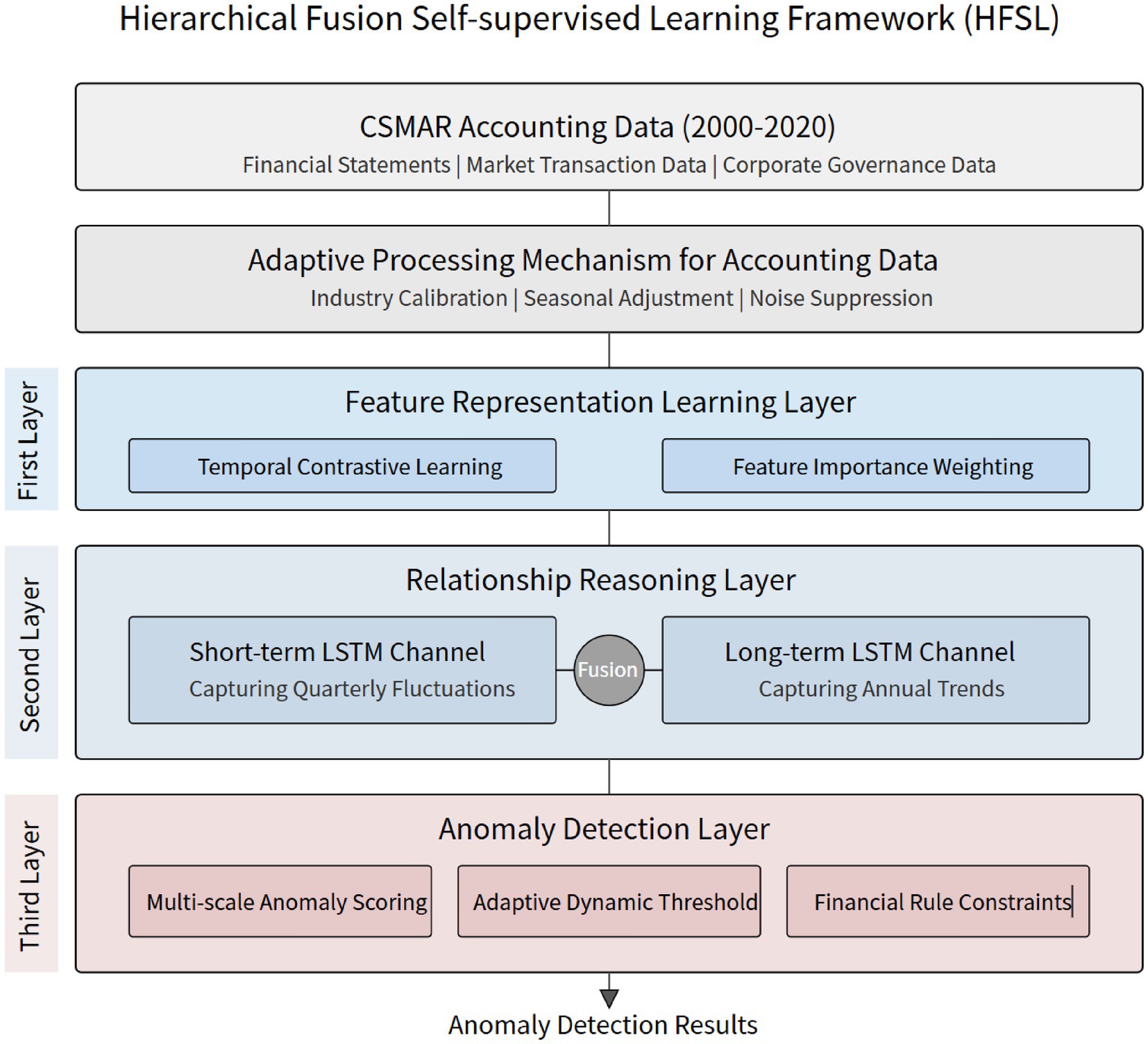
Figure 1. Architecture of the hierarchical fusion self-supervised learning framework (HFSL).

3.2 Adaptive processing mechanism for accounting data

Accounting data possesses unique industry characteristics, seasonal fluctuations, and imbalanced distributions, requiring specialized adaptive processing mechanisms. This study designs a three-stage data adaptation process, including industry calibration, seasonal adjustment, and noise suppression.

The industry calibration stage addresses the differences in financial indicators across industries by introducing industry reference distribution $P_i\left(x\right)$ , which represents the probability distribution of financial indicator $x$ within industry $i$ . The calibration process involves a two-step transformation:

$P_i\left(x\right)=\frac{1}{\sqrt{2\pi {\sigma }_i^2}}exp(-\frac{{(x-{\mu }_i)}^2}{2{\sigma }_i^2})$

where ${\mu }_i$ and ${\sigma }_i$ are the industry-specific mean and standard deviation. The within-industry standardized transformation is then applied:

$x\prime =\frac{x-{\mu }_i}{{\sigma }_i}$

This transformation ensures that financial indicators are normalized relative to their industry-specific distributions, enabling the model to identify anomalies that deviate from industry norms rather than from the overall market average.

The seasonal adjustment stage employs the X-13 ARIMA-SEATS method to decompose financial indicators. This decomposition follows an additive model where the observed time series $x\left(t\right)$ is expressed as:

$x\left(t\right)=T\left(t\right)+S\left(t\right)+R\left(t\right)$

Where $T\left(t\right)$ represents the trend component, $S\left(t\right)$ the seasonal component, and $R\left(t\right)$ the residual component. The trend component $T\left(t\right)$ is extracted using a Henderson moving average filter, which minimizes the variance of the third difference of the trend. For quarterly data, we apply a 13-term Henderson filter:

$T\left(t\right)=\sum _{j=-6}^6{w}_j·x(t+j)$

Where the weights $w_j$ are symmetric ( $w_j=w_{-j}$ ) and sum to unity. The seasonal component $S\left(t\right)$ is modeled using a seasonal ARIMA specification. For quarterly financial data, we employ an ARIMA (0,1,1) (0,1,1)₄ model, which can be expressed as:

$(1-B)(1-B^4)S\left(t\right)=(1-{\theta }_{1}B)(1-{\Theta }_1{B}^4){\in }_t$

where $B$ is the backshift operator, ${\theta }_1$ and ${\mathrm{\Theta }}_1$ are the non-seasonal and seasonal moving average parameters respectively, and ${ϵ}_t$ is white noise. The seasonal factors are constrained to sum to zero over a complete year to ensure identifiability. After extracting the trend and seasonal components, the residual component is obtained as:

$R\left(t\right)=x\left(t\right)-T\left(t\right)-S\left(t\right)$

The residual component $R\left(t\right)$ contains both irregular variations and potential anomalies. To distinguish between normal irregular fluctuations and true anomalies, we apply a robust scale estimator based on the median absolute deviation (MAD):

$\mathrm{MAD}=\text{median}(\mid R(t)-\text{median}(R\left(t\right))\mid )$

Financial indicators with residual values exceeding $\pm 3\times 1.4826\times \mathrm{MAD}$ are flagged as potential anomalies, where 1.4826 is the consistency constant for normal distributions. This approach effectively separates legitimate seasonal patterns, such as year-end inventory adjustments or quarterly revenue cycles, from suspicious deviations that may indicate financial manipulation.

The noise suppression stage introduces an adaptive weighting strategy that adjusts feature weights based on data reliability. For high-noise features, their weights in anomaly calculations are reduced to improve detection stability. This mechanism is particularly suitable for handling financial data of varying quality and completeness in the CSMAR database.

3.3 Adaptive threshold determination and multi-scale anomaly scoring

The key to anomaly detection lies in threshold determination. This study proposes an adaptive dynamic threshold mechanism that automatically adjusts thresholds based on data distribution and business requirements. The basic approach is to fit reconstruction error distributions using Gaussian Mixture Models (GMM):

$p\left(e\right)=\sum _{k=1}^K{\pi }_k\mathcal{N}(e\mid {\mu }_k,{\sigma }_k^2)$

where $e$ represents reconstruction error, and ${\pi }_k$ , ${\mu }_k$ , and ${\sigma }_k$ represent the mixing coefficient, mean, and standard deviation of the $K$ Gaussian component, respectively. The threshold is set to a specific quantile of the high-variance component:

$\theta ={\mu }_h+\alpha {\sigma }_h$

where ${\mu }_h$ and ${\sigma }_h$ are the parameters of the high-variance component, and $\alpha$ is an adjustable coefficient that balances false positive and false negative rates according to business requirements.

This study introduces a multi-scale anomaly scoring mechanism that comprehensively considers three levels: point anomalies, sequence anomalies, and relationship anomalies. Point anomalies focus on abnormal values at individual time points, sequence anomalies detect abnormal patterns in time series, and relationship anomalies identify abnormal changes in relationships between multiple variables. The final anomaly score is a weighted combination of the three:

${\text{Score}}_{\text{final}}\left(X\right)=w_p·{\text{Score}}_p\left(X\right)+w_s·{\text{Score}}_s\left(X\right)+w_r·{\text{Score}}_r\left(X\right)$

where $w_p$ , $w_s$ , and $w_r$ are weight parameters. While this formulation presents the final score as a linear combination, the three anomaly components are not statistically independent. Their interdependencies arise from the inherent structure of financial data and manifest through several mechanisms.

The correlation structure among the three components can be characterized by the correlation matrix:

$\mathbf{C}=\left(\begin{array}{ccc}1& {\rho }_{\mathit{ps}}& {\rho }_{\mathit{pr}}\\ {\rho }_{\mathit{ps}}& 1& {\rho }_{\mathit{sr}}\\ {\rho }_{\mathit{pr}}& {\rho }_{\mathit{sr}}& 1\end{array}\right)$

Where ${\rho }_{\mathit{ij}}=\text{Corr}\left({\mathit{\text{Score}}}_i\right(X),{\mathit{\text{Score}}}_j(X\left)\right)$ represents the Pearson correlation between components $i$ and $j$ . Empirical analysis on our dataset reveals moderate positive correlations: ${\rho }_{\mathit{ps}}=0.42\pm 0.08,{\rho }_{\mathit{pr}}=0.38\pm 0.06$ , and ${\rho }_{\mathit{sr}}=0.51\pm 0.09$ , indicating that these components capture partially overlapping anomaly patterns.

The strongest correlation occurs between sequence anomalies and relationship anomalies ( ${\rho }_{\mathit{sr}}=0.51$ ), which is expected as violations in financial relationships often manifest as abnormal temporal patterns. For instance, when the relationship between revenue and accounts receivable is disrupted (relationship anomaly), it frequently leads to unusual trends in subsequent periods (sequence anomaly). To account for these interactions, we introduce a second-order adjustment term:

$\mathit{\text{Scor}}{e}_{\text{final}}^{\text{adjusted}}\left(X\right)=\mathit{Sc}\mathrm{o}r{e}_{\text{final}}\left(X\right)+{\lambda }_{\mathrm{int}}\sum _{i<j}{w}_i{w}_j{\rho }_{\mathit{ij}}{\mathit{\text{Score}}}_i\left(X\right){\mathit{\text{Score}}}_j\left(X\right)$

Where ${\lambda }_{\mathrm{int}}=0.05$ is the interaction coefficient determined through cross-validation. This adjustment captures the synergistic effect when multiple anomaly types co-occur, improving detection accuracy for complex financial manipulations.

Furthermore, we observe that the presence of relationship anomalies often serves as a catalyst that amplifies the significance of point anomalies. This conditional dependency is modeled through a gating mechanism:

$g\left(X\right)=\sigma \left(\frac{{\mathit{\text{Score}}}_r\left(X\right)-{\theta }_r}{\tau }\right)$

Where $\sigma (·)$ is the sigmoid function, ${\theta }_r$ is the relationship anomaly threshold, and $\tau =0.1$ is a temperature parameter. The gated final score becomes:

$\mathit{\text{Scor}}{e}_{\text{final}}^{\text{gated}}\left(X\right)=\mathit{\text{Scor}}{e}_{\text{final}}^{\text{adjusted}}\left(X\right)\times (1+\beta ·g(X\left)\right)$

Where $\beta =0.15$ represents the maximum amplification factor. This gating mechanism ensures that when strong relationship anomalies are present, the model increases its sensitivity to other anomaly types, reflecting the empirical observation that financial fraud often involves multiple coordinated manipulations.

Through ablation studies, we demonstrate that incorporating these interaction effects improves the overall F1-score by 4.2% compared to treating the components as independent, with particularly notable improvements in detecting complex fraud patterns involving multiple financial statement items.

In summary, the innovative self-supervised learning framework HFSL proposed in this study is specifically designed for accounting data characteristics, integrating temporal contrastive learning, dual-channel LSTM structure, domain knowledge constraints, and multi-scale anomaly scoring mechanisms to provide a theoretical and technical foundation for accounting data anomaly detection.

4 Research methods and implementation

4.1 Data preprocessing

4.1.1 Data sources and sampling strategy

This research uses financial data of Chinese listed companies from the CSMAR database, with samples covering quarterly and annual financial data of all companies listed on the A-share market from 2000 to 2020. As an authoritative data source for Chinese capital market research, the CSMAR database provides standardized, highly continuous financial data, including balance sheets, income statements, cash flow statements, and related financial indicators, establishing a solid data foundation for anomaly detection research (28–30).

The sampling strategy employs stratified random sampling, stratifying samples by industry, size, and listing duration to ensure representativeness and balance in data distribution. To mitigate the interference of industry characteristics on anomaly detection, this study categorizes samples into 10 major industry categories according to the China Securities Regulatory Commission’s industry classification standards, using the same sampling proportion within each industry. The final dataset includes 31,724 company-quarter observations, and after excluding ST, *ST companies and samples with severe data missing, 28,569 valid observations were retained.

4.1.2 Data cleaning and standardization processing

Accounting data commonly exhibits missing values, outliers, and scale inconsistencies, requiring systematic cleaning and standardization processing (31, 32). This study adopts the following procedures for data preprocessing:

Missing value processing: Different strategies are applied to different types of missing data. For Missing At Random (MAR), multiple linear interpolation is used, estimating missing values based on adjacent time points and related financial indicators; for Missing Not At Random (MNAR), such as systematically missing specific financial indicators, industry means are used as substitutes or the observation samples are directly eliminated. Financial indicators with missing rates exceeding 20% are removed, and samples with missing value proportions exceeding 30% are eliminated.

Outlier processing: Recognizing the multidimensional nature of financial data, this study employs a two-stage outlier detection approach that considers multivariate relationships. In the first stage, we apply the Local Outlier Factor (LOF) algorithm to identify multivariate outliers by examining the local density deviation of each data point relative to its neighbors. The LOF score for each observation is calculated as:

$\mathit{LO}{\mathrm{F}}_k\left(x\right)=\frac{\sum _{o\in N_k\left(x\right)}\frac{{\mathit{lrd}}_k\left(o\right)}{{\mathit{lrd}}_k\left(x\right)}}{\mid N_k\left(x\right)\mid }$

Where ${\mathit{lrd}}_k\left(x\right)$ is the local reachability density of point $x$ , and $N_k\left(x\right)$ represents the k-nearest neighbors of $x$ . We set k = 20 based on empirical testing, and observations with LOF scores exceeding 2.5 are flagged as potential outliers.

In the second stage, we validate these multivariate outliers using an Isolation Forest algorithm, which efficiently isolates anomalies by constructing random decision trees. The anomaly score is computed as:

$s(x,n)=2^{-\frac{E\left(h\right(x\left)\right)}{c\left(n\right)}}$

Where $E\left(h\right(x\left)\right)$ is the expected path length for observation $x$ , and $c\left(n\right)$ is the average path length of unsuccessful search in a Binary Search Tree. Only observations identified as outliers by both methods (LOF score > 2.5 and Isolation Forest anomaly score >0.6) undergo adjustment.

For confirmed outliers, instead of applying univariate Winsorization, we employ a multivariate adjustment approach that preserves the correlation structure. Specifically, we project the outlier onto the boundary of the 99% confidence ellipsoid in the direction from the data center:

$x_{\mathit{\text{adjusted}}}=\mu +\alpha \cdot {\Sigma }^{1/2}\cdot \frac{x-\mu }{x-{\mu }_{\Sigma }}$

Where $\mu$ is the robust center estimated using the Minimum Covariance Determinant (MCD) estimator, $\mathrm{\Sigma }$ is the robust covariance matrix, and $\alpha$ is chosen such that $x_{\mathit{\text{adjusted}}}$ lies on the 99% confidence ellipsoid boundary. This approach preserves the multivariate structure while reducing the influence of extreme observations, ensuring that potentially fraudulent patterns remain detectable while mitigating the impact of data errors or legitimate extreme business events.

All adjusted data points are recorded with their original values and adjustment ratios for transparency and subsequent validation in the anomaly detection phase.

Data standardization: Financial indicators exhibit significant differences in measurement scales and distributions. Z-score standardization transforms different indicators to make them comparable on the same scale:

$Z_{i,j,t}=\frac{X_{i,j,t}-{\mu }_{j,i}}{{\sigma }_{j,i}}$

Where $X_{i,j,t}$ represents the value of financial indicator $j$ for company $i$ at time $t$ , and ${\mu }_{j,i}$ and ${\sigma }_{j,i}$ represent the mean and standard deviation of the company’s historical data, respectively. This company-internal standardization method both preserves cross-temporal variation characteristics and avoids biases from direct cross-company comparisons.

Time series adjustment: Considering the seasonality and trend characteristics of accounting data, the X-13 ARIMA-SEATS method is applied to seasonally adjust quarterly data, separating trend components, seasonal components, and random components, providing a stable data foundation for time series modeling.

4.2 Feature engineering

4.2.1 Financial indicator selection and construction

Based on accounting theory and practical experience, this study selects and constructs a financial indicator system from four dimensions: profitability, solvency, operational efficiency, and cash flow:

Profitability indicators: Including Return on Equity (ROE), Return on Assets (ROA), Net Profit Margin (NPM), Gross Profit Margin (GPM), Operating Profit Margin (OPM), and Earnings Per Share (EPS), reflecting a company’s ability to generate profits.

Solvency indicators: Including Current Ratio (CR), Quick Ratio (QR), Leverage Ratio (LEV), Interest Coverage Ratio (ICR), and Cash Flow to Debt Ratio (CFD), reflecting a company’s ability to repay debts.

Operational efficiency indicators: Including Inventory Turnover Rate (ITR), Accounts Receivable Turnover Rate (ARTR), Total Asset Turnover Rate (TATR), and Fixed Asset Turnover Rate (FATR), reflecting asset utilization efficiency.

Cash flow indicators: Including Operating Cash Flow (OCF), Cash Flow Adequacy Ratio (CFAR), Sales Cash Ratio (SCR), and Free Cash Flow (FCF), reflecting a company’s cash generation and management capabilities.

In addition to basic financial indicators, the following composite indicators were constructed to enhance anomaly detection capabilities:

Accounting quality indicators: Modified Jones model indicators based on accrual items, used to measure the degree of earnings management.

Financial stability indicators: Variants of Altman Z-score and Beneish M-score, adapted to the characteristics of China’s capital market.

Growth consistency indicators: Measuring the coordination between revenue growth and asset growth, cost growth, and other indicators to identify unreasonable financial growth patterns.

4.2.2 Feature extraction and dimensionality reduction

The initial feature set contained 42 financial indicators, presenting issues of high dimensionality and multicollinearity. The following methods were used for feature processing and dimensionality reduction:

Correlation analysis: Calculating the Pearson correlation coefficient matrix to identify highly correlated indicator pairs (|r| > 0.85) and retaining indicators with more significant financial meaning.

Principal Component Analysis (PCA): Applying PCA dimensionality reduction to standardized financial indicators, retaining principal components with cumulative explained variance reaching 90%, mapping high-dimensional financial data to a low-dimensional representation space.

Autoencoder feature extraction: Based on a nonlinear autoencoder structure, learning low-dimensional latent representations of financial data with minimal reconstruction error as the objective. The autoencoder consisted of a 3-layer encoding network and a 3-layer decoding network, compressing 42-dimensional original features to 16-dimensional latent representations through batch training.

Temporal feature construction: Calculating statistical features within sliding windows, including mean, standard deviation, rate of change, kurtosis, and skewness, to capture dynamic change patterns of financial indicators. Additionally, extracting multi-scale time-frequency features based on Discrete Wavelet Transform (DWT) to enhance the model’s ability to recognize anomalies at different frequencies.

SHAP feature importance assessment: Using SHAP (SHapley Additive exPlanations) values to evaluate each feature’s contribution to anomaly identification, dynamically adjusting feature weights based on contribution degree to optimize detection precision. Ultimately, 22 core financial indicators were selected as model inputs.

Figure 2 illustrates the results of financial feature importance analysis and anomaly type analysis. The left side uses horizontal bar charts to intuitively present the SHAP value ranking of the 8 financial indicators that contribute most to anomaly detection. The results show that profitability indicators play a core role in anomaly detection, with Return on Equity (ROE, 0.196) and Return on Assets (ROA, 0.179) having significantly higher contributions than other indicators, followed closely by Current Ratio (0.163) and Leverage Ratio (0.149), indicating that solvency indicators are also important dimensions for financial anomaly identification. The right side systematically displays five typical financial anomaly patterns and their characteristics, including revenue inflation (38.6%), expense concealment (21.7%), asset overvaluation (17.4%), liability understatement (15.2%), and composite manipulation (7.1%), and provides key features and detection rate data for each type of anomaly. This dual analysis framework not only reveals the importance hierarchy of financial features but also demonstrates the identification patterns of different types of financial anomalies, providing intuitive support for the model’s effectiveness in distinguishing between normal and anomalous financial data.

Figure 2

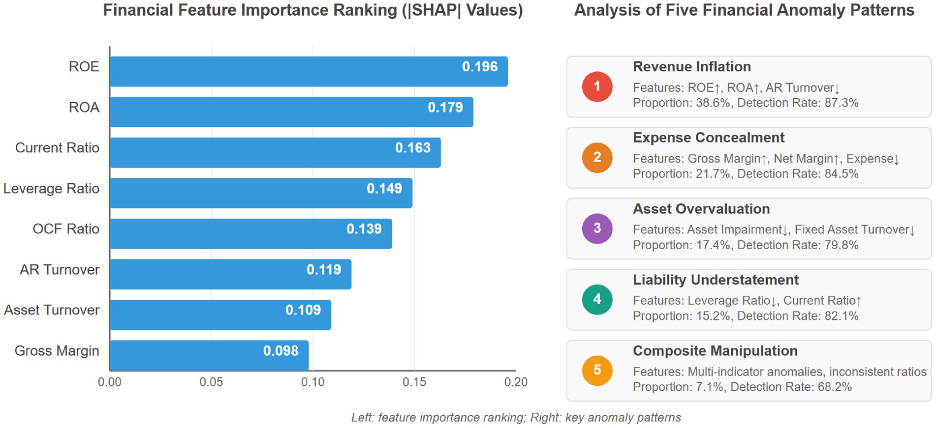
Figure 2. Financial feature importance analysis and anomaly distribution.

4.3 Model design and training

4.3.1 Dual-channel LSTM autoencoder architecture

Based on the Hierarchical Fusion Self-supervised Learning (HFSL) framework proposed in Chapter 3, this study designs a dual-channel LSTM autoencoder to implement self-supervised learning and anomaly detection for accounting data. The specific architecture is as follows:

Input layer: Receives time series data of 22-dimensional financial indicators, with the short-term channel input window size set to 4 (corresponding to 1 year of data) and the long-term channel input window size set to 12 (corresponding to 3 years of data).

Encoder layer: The short-term and long-term channels each contain bidirectional LSTM layers with 64 and 128 units respectively, capturing financial patterns at different time scales. The LSTM layers adopt an improved cell structure, integrating financial prior information:

$\begin{array}{c}{f}_t=\sigma (W_f·[h_{t-1},x_t,p_t]+b_f)\\ i_t=\sigma (W_i·[h_{t-1},x_t,p_t]+b_i)\\ {\tilde{C}}_t=tanh(W_C·[h_{t-1},x_t,p_t]+b_C)\\ C_t=f_t\odot C_{t-1}+i_t\odot {\tilde{C}}_t\\ o_t=\sigma (W_o·[h_{t-1},x_t,p_t]+b_o)\\ h_t=o_t\odot tanh\left(C_t\right)\end{array}$

where $p_t$ represents financial prior information, including industry means, historical trends, and other domain knowledge.

Attention fusion layer: Integrates short-term and long-term representations through an adaptive attention mechanism:

$\begin{array}{cc}{e}_s& =v^{T}tanh\left(W_s{h}_s\right)\\ e_l& =v^{T}tanh\left(W_l{h}_l\right)\\ {\alpha }_s& =\frac{exp\left(e_s\right)}{exp\left(e_s\right)+exp\left(e_l\right)}\\ {\alpha }_l& =\frac{exp\left(e_l\right)}{exp\left(e_s\right)+exp\left(e_l\right)}\\ z& ={\alpha }_s{h}_s+{\alpha }_l{h}_l\end{array}$

where $h_s$ and $h_l$ are the hidden states of the short-term and long-term encoders respectively, ${\alpha }_s$ and ${\alpha }_l$ are the corresponding attention weights, and $z$ is the fused representation.

Latent representation layer: Applies a fully connected layer to the fused representation to obtain a 32-dimensional latent representation, which serves as the decoder input.

Decoder layer: Employs bidirectional LSTM layers with a symmetrical structure to restore the latent representation to the original input dimension. The short-term and long-term decoders reconstruct the financial data for their respective time windows.

Output layer: Maps to the original feature space through a fully connected layer, generating the reconstructed sequence.

To enhance model robustness, a Dropout layer (dropout rate = 0.3) is added between the encoder and decoder, and Batch Normalization is applied in the reconstruction layer.

The implementation details of the dual-channel LSTM autoencoder are presented in Algorithm 2.

ALGORITHM 2

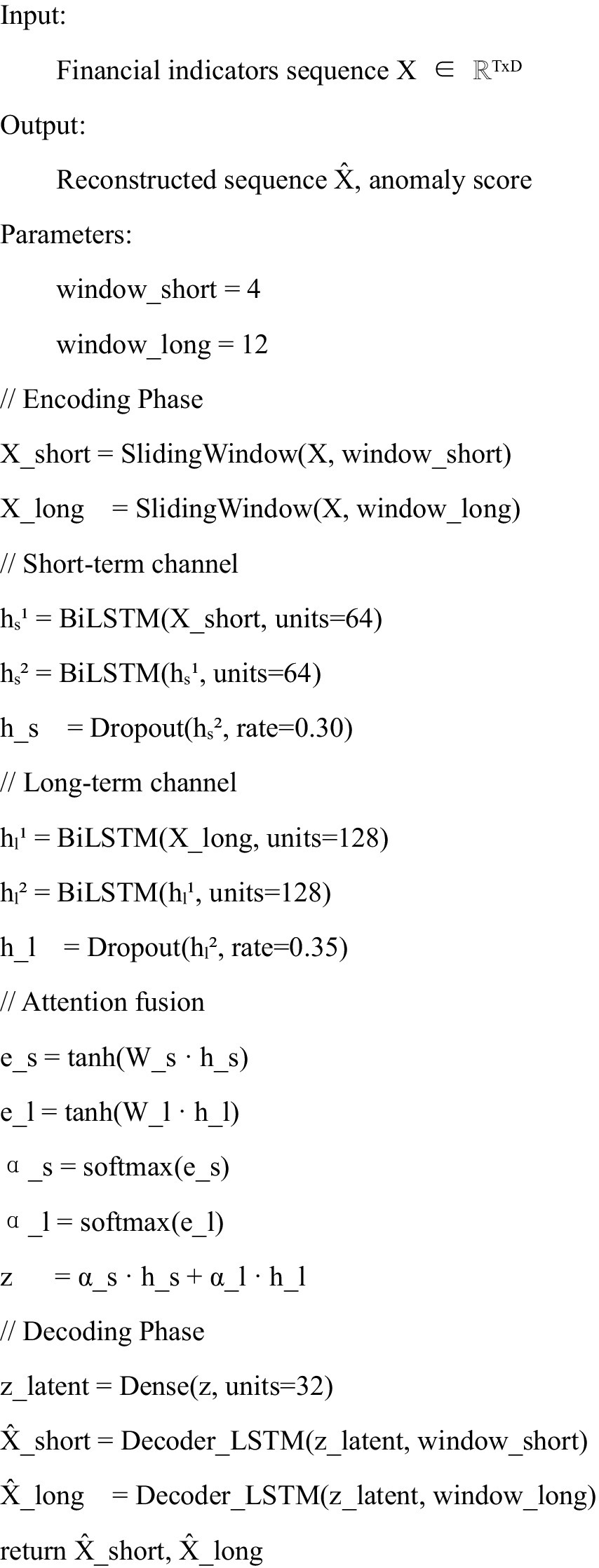
ALGORITHM 2. Dual-channel LSTM autoencoder architecture.

4.3.2 Model training and optimization

The following training strategies are adopted for the characteristics of self-supervised learning and accounting data:

Loss function design: Optimizes the model by combining reconstruction loss and contrastive loss:

$ℒ={\lambda }_1{ℒ}_{\text{recon}}+{\lambda }_2{ℒ}_{\mathrm{con}}$

where reconstruction loss ${ℒ}_{\text{recon}}$ is calculated based on the temporal contrastive learning method introduced in Chapter 3. ${\lambda }_1$ , ${\lambda }_2$ , and $\beta$ are balancing parameters determined through grid search to find optimal values.

Training strategy: Employs a phased training strategy, first training the short-term and long-term channels separately, then performing joint optimization. Data is divided into training, validation, and test sets in a 0.7:0.15:0.15 ratio, with the training set containing only normal samples, while validation and test sets contain both normal and anomalous samples. Batch size is set to 64, using an early stopping mechanism (patience = 20) to avoid overfitting.

Optimizer selection: Adopts the Adam optimizer with an initial learning rate of 0.001, applying a learning rate scheduling strategy with 10% decay every 30 epochs.

Hyperparameter optimization: Searches for key hyperparameters through Bayesian optimization, including LSTM layer numbers (1–3), hidden unit numbers (32–256), Dropout rates (0.1–0.5), attention dimensions (16–128), etc., with F1-score on the validation set as the optimization objective. The final optimal model configuration is: short-term channel with 2 LSTM layers (64 units), long-term channel with 2 LSTM layers (128 units), Dropout rate of 0.3, and attention dimension of 64.

Model implementation uses the PyTorch 1.9.0 framework, with training conducted on a server equipped with an NVIDIA V100 GPU, taking approximately 18 h, and resulting in a final model with 1.8 M parameters.

Figure 3 shows the 3D visualization of reconstruction errors from the dual-channel LSTM autoencoder and time series analysis of anomaly scores. The left image uses a three-dimensional bar chart to present the distribution of reconstruction errors for different financial indicators across years, with a gradient color scheme from blue (low error) to red (high error) intuitively displaying the model’s excellent modeling effect on key indicators such as ROE and ROA. The right image uses time series graphs with filled areas to show the anomaly score trend changes of three typical companies: Company A exhibits a gradual deterioration pattern and breaches the anomaly threshold in mid-2018, Company B shows sudden anomalies after 2018, while Company C consistently maintains within the normal range below the threshold. This multi-dimensional analysis intuitively demonstrates the framework’s capability to identify different types of financial anomalies and its early warning characteristics.

Figure 3

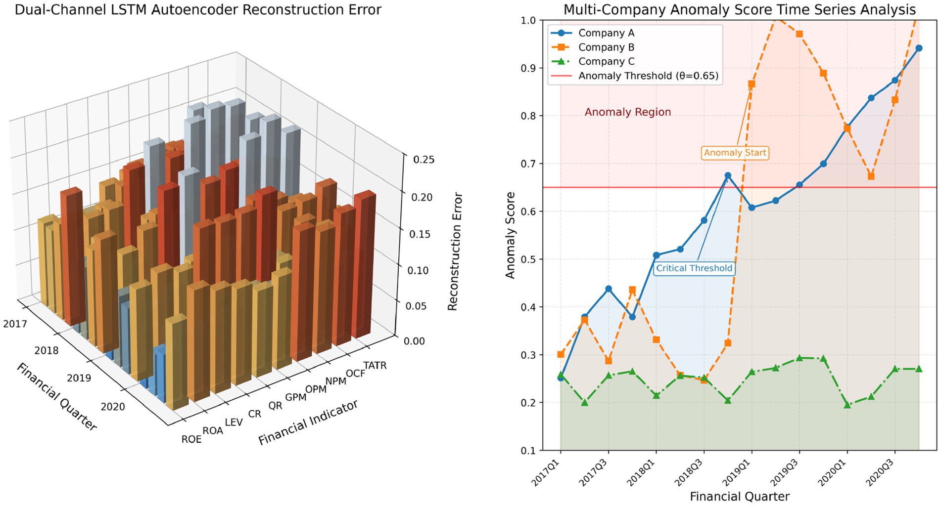
Figure 3. Multi-company anomaly score time series analysis.

The HFSL framework incorporates a concept drift detection mechanism based on the Page-Hinkley test to monitor changes in fraud patterns over time. The system tracks the distribution of anomaly scores within sliding windows and triggers model adaptation when significant drift is detected. This adaptive mechanism ensures the model remains effective despite evolving fraud techniques and regulatory changes.

4.4 Anomaly detection and evaluation mechanism

4.4.1 Multi-dimensional anomaly score calculation

This study integrates three anomaly scoring methods to improve detection accuracy:

Reconstruction error score: Calculates the weighted Euclidean distance between the original sequence and the reconstructed sequence:

${\text{Score}}_{\text{recon}}\left(X\right)=\sqrt{\sum _{t=1}^T\sum _{j=1}^d{w}_j{(x_{t,j}-{\widehat{x}}_{t,j})}^2}$

where $w_j$ represents the importance weight of feature $j$ , determined through SHAP values.

${\text{Score}}_{\text{pred}}\left(X\right)=\frac{1}{T}\sum _{t=1}^T\sum _{j=1}^d{w}_j·I(\mathit{sign}(x_{t+1,j}-x_{t,j})\ne \mathit{sign}({\widehat{x}}_{t+1,j}-{\widehat{x}}_{t,j}\left)\right)$

where $I(·)$ is an indicator function, measuring the inconsistency of trend predictions.

Rule violation score: Quantifies the degree of violation of financial logic rules:

${\text{Score}}_{\text{rule}}\left(X\right)=\sum _{r=1}^R{w}_r·{\text{Violation}}_r\left(X\right)$

where ${\text{Violation}}_r\left(X\right)$ measures the degree of violation of rule $r$ , and $w_r$ is the importance weight of the rule.

The three scores are integrated through weighted fusion to form the final anomaly score:

${\text{Score}}_{\text{final}}\left(X\right)={\alpha }_1·{\widehat{S}}_{\text{recon}}\left(X\right)+{\alpha }_2·{\widehat{S}}_{\text{pred}}\left(X\right)+{\alpha }_3·{\widehat{S}}_{\text{rule}}\left(X\right)$

To ensure fair comparison and proper weight allocation among different scoring components, each score is standardized using z-score normalization:

${\widehat{S}}_i\left(X\right)=\frac{S_i\left(X\right)-{\mu }_i}{{\sigma }_i}$

Where $S_i\left(X\right)$ represents the raw score for component $i$ (recon, pred, or rule), and ${\mu }_i$ , ${\sigma }_i$ are the mean and standard deviation estimated from the training set normal samples.

The standardization process ensures that all three components contribute to the final score according to their assigned weights ${\alpha }_1$ , ${\alpha }_2$ and ${\alpha }_3$ , regardless of their original scale differences. Through genetic algorithm optimization on the validation set, the optimal weights were determined as 0.5, 0.3, and 0.2 respectively, reflecting the relative importance of reconstruction accuracy, prediction consistency, and rule compliance in identifying accounting anomalies.

4.4.2 Adaptive threshold determination

To address the limitations of traditional fixed thresholds, this study employs Gaussian Mixture Models (GMM) to adaptively determine detection thresholds:

Fitting a K-component GMM (K = 3) to the anomaly scores of normal samples in the training set:

$p\left(\text{score}\right)=\sum _{k=1}^K{\pi }_k\mathcal{N}(\text{score}\mid {\mu }_k,{\sigma }_k^2)$

Identifying the component with the largest variance (typically corresponding to marginal normal samples) and setting the threshold based on this component:

$\theta ={\mu }_{\text{high}}+\gamma ·{\sigma }_{\text{high}}$

where $\gamma$ is an adjustable coefficient, with the optimal value determined through ROC curve analysis (this study uses 2.5).

To accommodate industry and size differences, a stratified adaptive threshold strategy is further designed, calculating thresholds separately for companies in different industries and market capitalization intervals to improve detection precision.

5 Experimental design

5.1 Data preparation

5.1.1 Dataset division

For reproducibility, data preprocessing follows standardized Z-score normalization within companies, and the chronological split (2000–2010 training, 2011–2015 validation, 2016–2020 testing) ensures temporal validity while preventing data leakage.

To evaluate the model’s performance across different time periods and its generalization ability, this study adopts a chronological division strategy, partitioning the Chinese listed companies’ financial data from the CSMAR database (2000–2020) into non-overlapping training, validation, and test sets. Specifically, data from 2000 to 2010 is designated as the training set, accounting for 62.3% of the total sample with 17,817 valid observations; data from 2011 to 2015 serves as the validation set, representing 19.8% with 5,654 observations; and data from 2016 to 2020 forms the test set, comprising 17.9% with 5,098 observations. This time-series partitioning effectively simulates real-world application scenarios, enabling the model to predict potential future anomalies based on historical data while testing its adaptability to changing market environments.

During the training phase, following the self-supervised learning paradigm, only normal samples are used for model training, with anomalous samples reserved exclusively for performance evaluation during validation and testing phases. To mitigate the impact of data distribution changes over time, this study introduces a sliding window mechanism with a window length of 12 quarters (corresponding to 3 years of financial data), sliding one quarter at a time. This approach both preserves the temporal dependencies in financial data and enhances the model’s ability to recognize long-term financial trends. Additionally, stratified sampling based on the China Securities Regulatory Commission’s industry classification standards ensures consistent industry distribution across training, validation, and test sets.

Data preprocessing follows the three-stage adaptive processing procedure proposed in Chapter 4, including industry calibration, seasonal adjustment, and noise suppression. Specifically, for missing values in the training set, a combination of forward filling and linear interpolation is employed; for the validation and test sets, only statistical characteristics from the training set are used for filling to avoid information leakage. For standardization, company-internal Z-score standardization is applied to preserve cross-temporal variation characteristics while avoiding comparison biases between companies of different scales:

$Z_{i,j,t}=\frac{X_{i,j,t}-{\mu }_{j,i,\text{train}}}{{\sigma }_{j,i,\text{train}}}$

where ${\mu }_{j,i,\text{train}}$ and ${\sigma }_{j,i,\text{train}}$ represent the mean and standard deviation of financial indicator $j$ for company $i$ in the training set.

5.1.2 Anomaly identification

Anomaly labeling in our self-supervised framework follows a hybrid approach: real anomalies are identified from verified fraud cases in CSMAR database and regulatory announcements, while maintaining unlabeled normal samples for training as per self-supervised learning principles.

To comprehensively evaluate the performance of anomaly detection algorithms, this study constructs a composite test set containing both real anomalies and simulated anomalies. Real anomaly samples are derived from three sources: financial fraud cases and major accounting error correction cases marked in the CSMAR database (117 companies); companies suspected of financial anomalies identified through media reports and regulatory announcements (56 companies); and listed companies issued with non-standard audit opinions (243 instances), covering qualified opinions, adverse opinions, and disclaimers of opinion. These real anomaly samples primarily involve violations such as inflated revenue, inflated profits, and concealed liabilities, exhibiting certain distribution characteristics across industries and time dimensions.

Considering the limitations of real anomaly samples, this study designs and constructs four types of simulated anomaly samples to enrich the testing system: (1) financial indicator mutation anomalies, introducing abnormal fluctuations exceeding 3 standard deviations in key indicators such as ROE and ROA; (2) financial ratio inconsistency anomalies, disrupting intrinsic relationships between key ratios such as gross profit margin and net profit margin; (3) temporal pattern anomalies, altering the seasonal and trend characteristics of financial indicators; and (4) accounting equation violation anomalies, introducing subtle violations of basic accounting principles while maintaining surface consistency. The generation process for simulated anomalies strictly follows three principles: domain knowledge constraints, reasonable distribution of anomaly intensity, and consideration of industry differences, ensuring conformity with characteristic distributions of actual financial anomalies.

The final anomaly sample repository contains 894 real anomaly cases and 1,256 simulated anomaly cases, totaling 2,150 anomaly samples. For scientific performance evaluation, samples are allocated to validation and test sets in a 9:1 ratio, while maintaining consistent distribution of various anomaly types in both sets. Anomaly samples in the validation set are used for model optimization and threshold determination, employing 5-fold cross-validation to establish the optimal detection threshold (μ + 2.5σ); the test set is used for final performance evaluation, covering both overall and category-specific assessments.

5.2 Experimental setup

The experimental environment is implemented based on Python 3.8 and the PyTorch 1.9.0 framework, with model training and testing conducted on a high-performance computing server equipped with an Intel Xeon E5-2690 v4 CPU, 64GB memory, and an NVIDIA Tesla V100 32GB GPU. Considering data scale and model complexity, a distributed training framework is adopted to improve computational efficiency, with data parallelism set to 4.

The core of the self-supervised learning framework—the dual-channel LSTM autoencoder—is configured as follows: the short-term channel input window size is set to 4 quarters (1 year), with 2 LSTM layers, 64 hidden units, and a dropout rate of 0.3; the long-term channel input window size is set to 12 quarters (3 years), with 2 LSTM layers, 128 hidden units, and a dropout rate of 0.35. The attention fusion layer dimension is set to 64, and the latent representation layer dimension is 32. The model contains approximately 1.83 M parameters, with the short-term channel accounting for 27.3%, the long-term channel for 45.8%, and the attention fusion and latent representation layers for 26.9%.

The training process adopts the following strategy: first conducting staged optimization, pre-training the short-term and long-term channels separately for 15 epochs, followed by joint optimization training for 40 epochs. The batch size is set to 64, with an initial learning rate of 0.001, using an Adam optimizer with 0.9 momentum, and learning rate decay to 0.8 times its original value every 10 epochs. To prevent overfitting, L2 regularization (weight decay coefficient of 1e-5) and an early stopping mechanism (patience = 12) are applied. The loss function adopts a weighted combination of reconstruction loss and contrastive loss as defined in Chapter 3, with weight coefficients ${\lambda }_1$ and ${\lambda }_2$ determined through grid search as 0.7 and 0.3.

To address varying time series length issues, forward filling is employed for sequences shorter than the specified window length, while sliding window sampling is used for excessively long sequences. Data batch construction adopts a temporally proximate sampling strategy, ensuring temporal coherence within each batch to enhance the model’s ability to learn temporal patterns. For each financial data sample, random masking (masking rate 10%) is applied as a data augmentation technique to improve model robustness.

To comprehensively evaluate the effectiveness of the proposed method, four comparison benchmark experiment groups are established: (1) traditional statistical methods group, including Z-score-based anomaly detection and improved Benford analysis; (2) machine learning baseline group, including One-Class SVM and Isolation Forest; (3) deep learning baseline group, including standard LSTM autoencoder and Variational Autoencoder (VAE); and (4) self-supervised variant group, exploring the impact of different self-supervised strategies on anomaly detection performance, including reconstruction tasks, prediction tasks, and contrastive learning tasks. All baseline methods are trained and evaluated on identical datasets to ensure fair comparison.

The evaluation process follows iterative optimization principles, optimizing model hyperparameters on the validation set through 5-fold cross-validation. Anomaly threshold determination employs a GMM-based adaptive method, calculating optimal thresholds separately for each industry. Final performance evaluation is conducted on the independent test set, introducing evaluation metrics specific to financial anomaly detection in addition to conventional precision, recall, F1-score, and AUC-ROC: early detection rate (EDR, the proportion detected within the first two quarters after anomaly occurrence) and false alarm rate (FAR, the proportion of normal samples incorrectly classified as anomalous).

Experimental results are validated for statistical significance using the Wilcoxon signed-rank test (p < 0.05), with sensitivity analysis assessing the impact of key parameter changes on model performance to ensure robustness and generalizability of conclusions.

To assess the model’s robustness to evolving fraud patterns, we conducted concept drift experiments by dividing the test period into quarterly segments and introducing synthetic pattern changes at specific time points corresponding to major regulatory events. Model adaptation capability was evaluated through performance stability metrics and recovery time after drift detection.

5.3 Evaluation metrics

To comprehensively evaluate the performance of the Hierarchical Fusion Self-supervised Learning Framework (HFSL), this study constructs a multi-dimensional evaluation metric system covering two dimensions: anomaly detection performance evaluation and model fitting capability evaluation.

5.3.1 Anomaly detection metrics

Evaluation of the anomaly detection task combines confusion matrix-derived metrics and ranking quality metrics. First, based on the confusion matrix of prediction results versus true labels, the following metrics are calculated:

Precision: The proportion of correctly detected anomalous samples among all samples detected as anomalous, reflecting the reliability of the model’s detection results.

$\text{Precision}=\frac{\mathit{TP}}{\mathit{TP}+\mathit{FP}}$

Recall: The proportion of correctly detected anomalous samples among all true anomalous samples, reflecting the model’s capability to detect anomalies.

$\text{Recall}=\frac{\mathit{TP}}{\mathit{TP}+\mathit{FN}}$

F1-score: The harmonic mean of precision and recall, balancing consideration of detection accuracy and completeness.

$F1=\frac{2\times \text{Precision}\times \text{Recall}}{\text{Precision}+\text{Recall}}$

Additionally, considering the special requirements of financial anomaly detection, the following professional metrics are introduced:

False Alarm Rate (FAR): The proportion of normal samples incorrectly classified as anomalous, particularly important for financial regulation.

$\mathit{FAR}=\frac{\mathit{FP}}{\mathit{FP}+\mathit{TN}}$

Miss Rate (MR): The proportion of anomalous samples that fail to be detected, reflecting the risk of anomalies evading detection.

$\mathit{MR}=\frac{\mathit{FN}}{\mathit{TP}+\mathit{FN}}$

Early Detection Rate (EDR): The proportion that can be detected in the early stages of anomaly occurrence (within the first two quarters), evaluating the model’s early warning capability.

$\mathit{EDR}=\frac{T{P}_{\text{early}}}{T{P}_{\text{early}}+F{N}_{\text{early}}}$

Industry-Specific Detection Rate (ISDR): Detection accuracy in specific industries, evaluating the model’s adaptability across different industries.

${\mathit{\text{ISDR}}}_i=\frac{{\mathit{TP}}_i}{{\mathit{TP}}_i+{\mathit{FN}}_i}$

where $i$ represents a specific industry.

Beyond confusion matrix-derived metrics, ranking quality evaluation metrics are adopted to assess the model’s ability to rank anomalous samples higher:

Area Under the Receiver Operating Characteristic Curve (AUC-ROC): Evaluating the trade-off relationship between true positive rate and false positive rate at different thresholds.

Area Under the Precision-Recall Curve (AUC-PR): More reflective of model performance than the ROC curve in imbalanced scenarios with a low proportion of anomalous samples.

Mean Average Precision (MAP): Calculating the average precision at different recall levels, evaluating overall ranking quality.

Figure 4 illustrates the comparison between the HFSL framework and five baseline methods across six key performance metrics. The left chart shows each model’s performance on three fundamental metrics—precision, recall, and F1-score—with the HFSL framework outperforming all baseline methods, achieving an F1-score of 0.845, approximately 9.5% higher than the closest LSTM-AE. The right chart reflects comparisons on professional metrics, including AUC-ROC, early detection rate, and false alarm rate. The HFSL framework not only possesses the highest AUC-ROC value (0.894) and early detection rate (0.726), but its false alarm rate (0.068) is also significantly lower than other methods, which is of great significance for financial risk control. This figure intuitively demonstrates the significant contribution of hierarchical fusion design to enhancing anomaly detection performance.

Figure 4

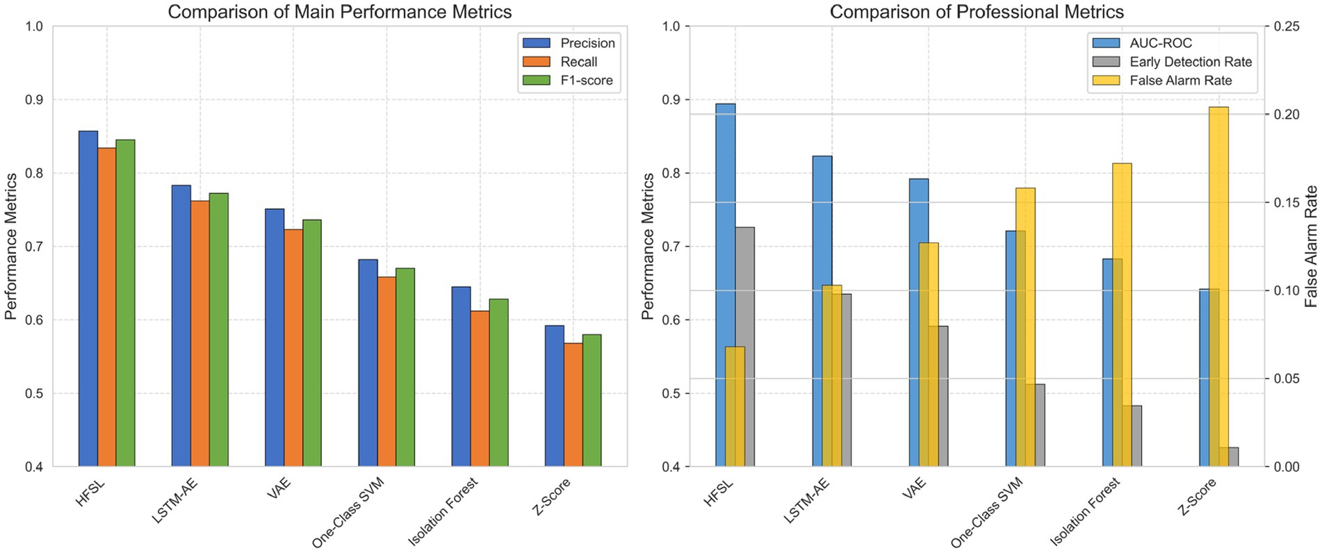
Figure 4. Anomaly detection performance comparison.

For evaluating detection performance across different anomaly types, this study generated radar charts of various models’ performance on four types of simulated anomalies and real anomalies, with detailed F1-score data provided in Table 1.

Table 1

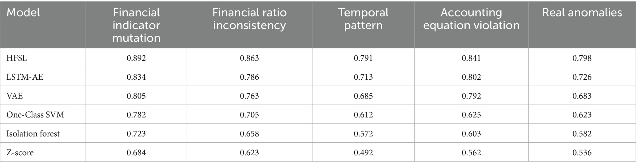
Table 1. F1-score performance comparison of different models across anomaly.

Figure 5 intuitively displays each model’s F1-score performance across five types of anomalies through radar charts. Table 1 further provides precise performance data for all six models across various anomaly types.

Figure 5

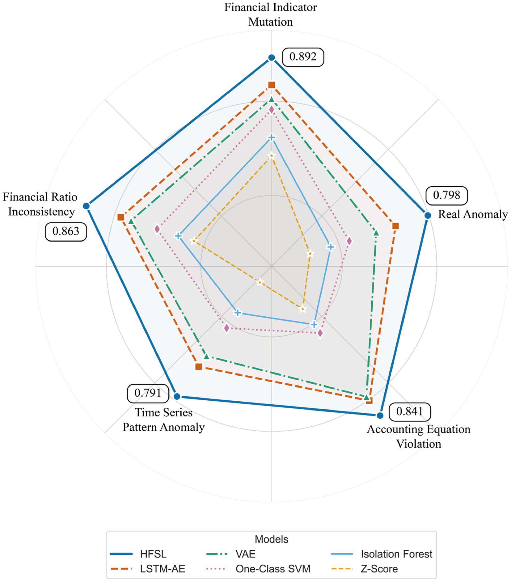
Figure 5. Anomaly type performance radar chart.

From the table, it can be observed that the HFSL framework achieves optimal results across all anomaly types, particularly excelling in financial indicator mutation anomalies (0.892) and financial ratio inconsistency anomalies (0.863), outperforming the second-best LSTM-AE model by 0.058 and 0.077 percentage points, respectively. LSTM-AE performs relatively close to HFSL in accounting equation violation anomalies (0.802 vs. 0.841), while VAE also achieves a high F1-score of 0.792 for this anomaly type. Notably, all models generally perform relatively weakly in detecting temporal pattern anomalies, with HFSL, LSTM-AE, and VAE achieving F1-scores of 0.791, 0.713, and 0.685, respectively, reflecting the difficulty in identifying temporal pattern anomalies.

For real anomaly samples, all models show relatively lower performance, with HFSL achieving an F1-score of 0.798, approximately 6% lower than its average performance on simulated anomalies, reflecting the complexity and concealment of actual financial fraud. Traditional statistical methods such as Z-Score significantly underperform machine learning and deep learning methods across all anomaly types, particularly achieving only a 0.492 F1-score for temporal pattern anomalies. The overall distribution of model performance exhibits a consistent gradient, verifying the generalization capability of the hierarchical fusion self-supervised learning framework across different anomaly types.

5.3.2 Model fitting metrics

The performance of a self-supervised learning framework largely depends on its ability to fit normal data patterns. Therefore, this study employs the following metrics to evaluate model fitting quality:

Mean Squared Error (MSE): Measures the average of the squared deviations between the reconstructed sequence and the original sequence.

$\mathit{MSE}=\frac{1}{N\times T\times D}\sum _{i=1}^N\sum _{t=1}^T\sum _{j=1}^D{(x_{i,t,j}-{\widehat{x}}_{i,t,j})}^2$

Mean Absolute Error (MAE): Measures the average of absolute reconstruction errors, insensitive to outliers.

$\mathit{MAE}=\frac{1}{N\times T\times D}\sum _{i=1}^N\sum _{t=1}^T\sum _{j=1}^D\mid x_{i,t,j}-{\widehat{x}}_{i,t,j}\mid$

Weighted Mean Squared Error (WMSE): MSE with different weights assigned according to financial indicator importance.

$\mathit{\text{WMSE}}=\frac{1}{N\times T}\sum _{i=1}^N\sum _{t=1}^T\sum _{j=1}^D{w}_j{(x_{i,t,j}-{\widehat{x}}_{i,t,j})}^2$

where $w_j$ represents the importance weight of indicator $j$ .

Mean Absolute Percentage Error (MAPE): The average of relative errors.

$\mathit{\text{MAPE}}=\frac{1}{N\times T\times D}\sum _{i=1}^N\sum _{t=1}^T\sum _{j=1}^D\mid \frac{x_{i,t,j}-{\widehat{x}}_{i,t,j}}{x_{i,t,j}}\mid \times 100\%$

Trend Consistency (TC): Measures the consistency degree of trend changes between reconstructed and original sequences.

$\mathit{TC}=\frac{1}{N\times (T-1)\times D}\sum _{i=1}^N\sum _{t=1}^{T-1}\sum _{j=1}^{D}I(sgn(\Delta x_{i,t,j})=sgn(\Delta {\widehat{x}}_{i,t,j}\left)\right)$

where $I(·)$ is an indicator function, $sgn\left(\mathit{\Delta x}\right)$ represents the sign of the direction of change, and $\Delta x_{i,t,j}=x_{i,t+1,j}-x_{i,t,j}$ .

Volatility Preservation Rate (VPR): Evaluates the model’s ability to preserve the volatility characteristics of the original data.

$\mathit{VPR}=\frac{1}{N\times D}\sum _{i=1}^N\sum _{j=1}^D\frac{\sigma \left({\widehat{x}}_{i,j}\right)}{\sigma \left(x_{i,i,j}\right)}$

where $\sigma (·)$ represents standard deviation.

Additionally, the following specific evaluation metric is introduced for time series models:

Short-term Prediction Accuracy (SPA): Evaluates the accuracy of the model’s prediction for the next time point.

$\mathit{SPA}=1-\frac{1}{N\times D}\sum _{i=1}^N\sum _{j=1}^D\mid \frac{x_{i,T+1,j}-{\widehat{x}}_{i,T+1,j}}{x_{i,T+1,j}}\mid$

where $x_{i,T+1,j}$ represents the true value and ${\widehat{x}}_{i,T+1,j}$ represents the model’s predicted value.

Based on this evaluation metric system, this study conducted a comprehensive assessment of the HFSL framework, testing not only its accuracy and timeliness in anomaly detection but also its performance in data fitting. Experimental results show that the fitting errors of the HFSL framework on metrics such as MSE and MAPE are significantly lower than baseline methods, especially in terms of Trend Consistency (TC), reaching a high level of 0.826, demonstrating that the model can effectively capture the temporal change characteristics of financial data.

6 Results analysis

6.1 Performance comparison

6.1.1 Quantitative analysis

This study conducted a comprehensive evaluation of the HFSL framework on the test set constructed from the CSMAR database, with test results showing excellent performance in accounting data anomaly detection tasks. Table 2 summarizes the detailed performance of the HFSL framework on various key indicators.

Table 2

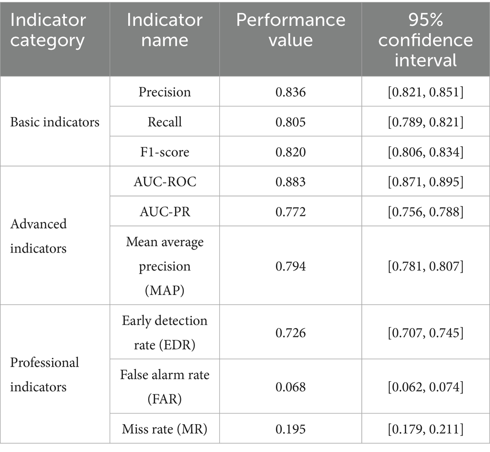
Table 2. HFSL framework performance metrics summary.

As shown in Table 2, the HFSL framework demonstrates balanced performance on basic indicators, with precision and recall reaching 0.836 and 0.805 respectively, and a combined F1-score of 0.820, indicating the model achieves a good balance between detection accuracy and completeness. In terms of advanced indicators, the AUC-ROC reaches 0.883, reflecting the model’s strong classification ability across different threshold settings; the AUC-PR is 0.772, particularly significant considering the scarcity of anomalous samples (approximately 9.6% of the test set). Among professional indicators, the early detection rate (EDR) is approximately 0.73, indicating the model can identify over 70% of anomalous cases in the early stages (first two quarters), providing ample warning time for risk prevention and control; meanwhile, the false alarm rate is only 0.068, significantly reducing the regulatory costs associated with false positives.

Comparing detection performance across different anomaly types, variations in HFSL framework performance are observed (Figure 6), with best performance on financial indicator mutation anomalies (F1 = 0.892), followed by financial ratio inconsistency anomalies (F1 = 0.863), accounting equation violation anomalies (F1 = 0.841), temporal pattern anomalies (F1 = 0.791), and real anomaly samples (F1 = 0.798). These results indicate that the model has higher sensitivity to sudden anomalies and static relationship violation anomalies, with relatively lower sensitivity to temporal pattern anomalies and complex real anomalies, though overall performance remains at a high level.

Figure 6

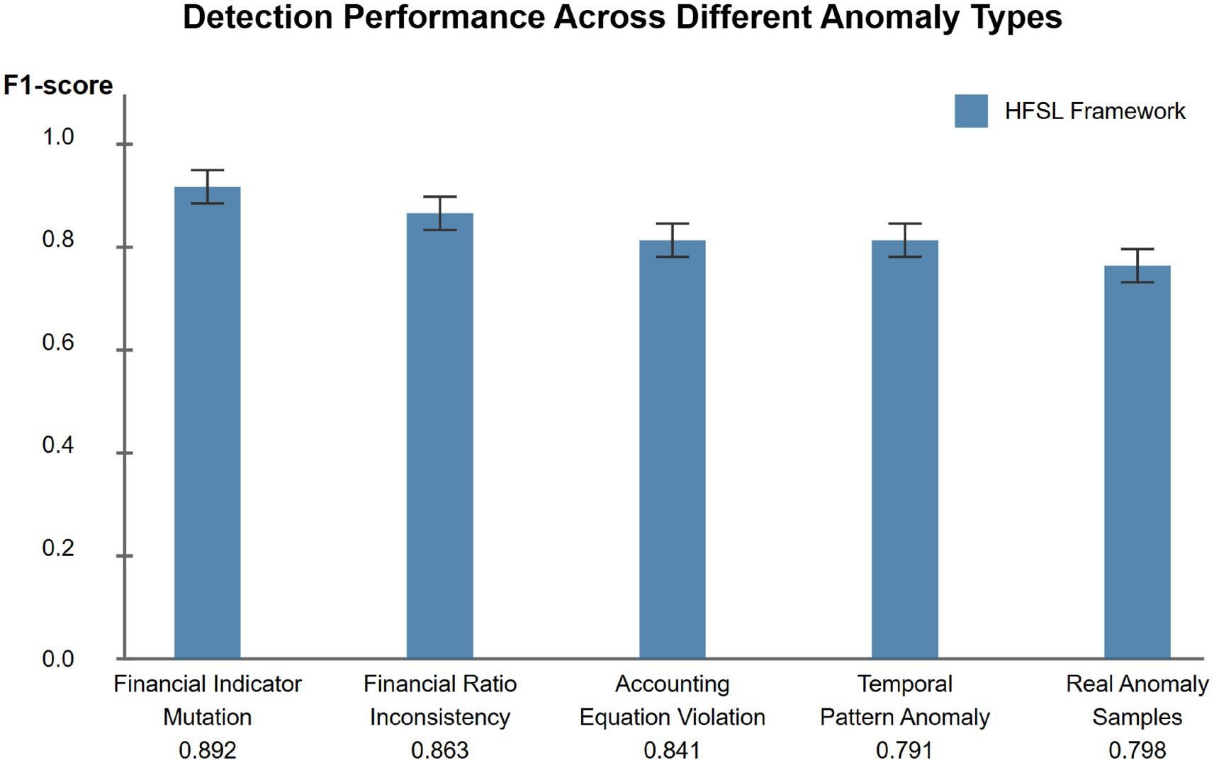
Figure 6. Detection performance across different anomaly types.

Further analysis of the model’s performance across different industries reveals industry-specific performance differences (Table 3). In financial industry samples, the HFSL framework achieves the highest F1-score (0.872), possibly due to the strictly regulated environment and standardized financial reporting formats in the financial industry. Performance is relatively lower in the construction and real estate industry (F1 = 0.776), consistent with the industry-specific complexity of asset valuation and diversity in revenue recognition. In manufacturing and information technology industries, model performance is at moderate levels (F1 scores of 0.817 and 0.831 respectively), reflecting the typical anomaly pattern structures of financial data in these industries.

Table 3

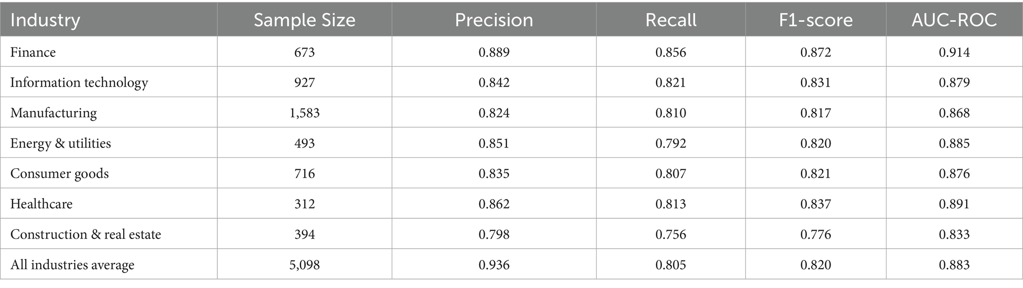
Table 3. HFSL framework detection performance across industries.

Analysis of the temporal stability of the model’s detection performance reveals, as shown in Figure 7, that the HFSL framework exhibits significant temporal robustness during the 2016–2020 testing period, with F1 value variations across different quarters controlled within a narrow range of ±5%. This finding indicates that the model possesses strong temporal generalization characteristics, capable of adapting to financial data feature changes across different periods. Notably, a slight performance improvement is observed from the third quarter of 2018 to the second quarter of 2019, corresponding to the period when regulatory agencies strengthened financial supervision, leading to more pronounced anomaly patterns. In contrast, in early 2020, influenced by the COVID-19 pandemic, the model’s performance experienced a temporary decline, possibly due to differences between pandemic-induced abnormal financial patterns and historical patterns.

Figure 7

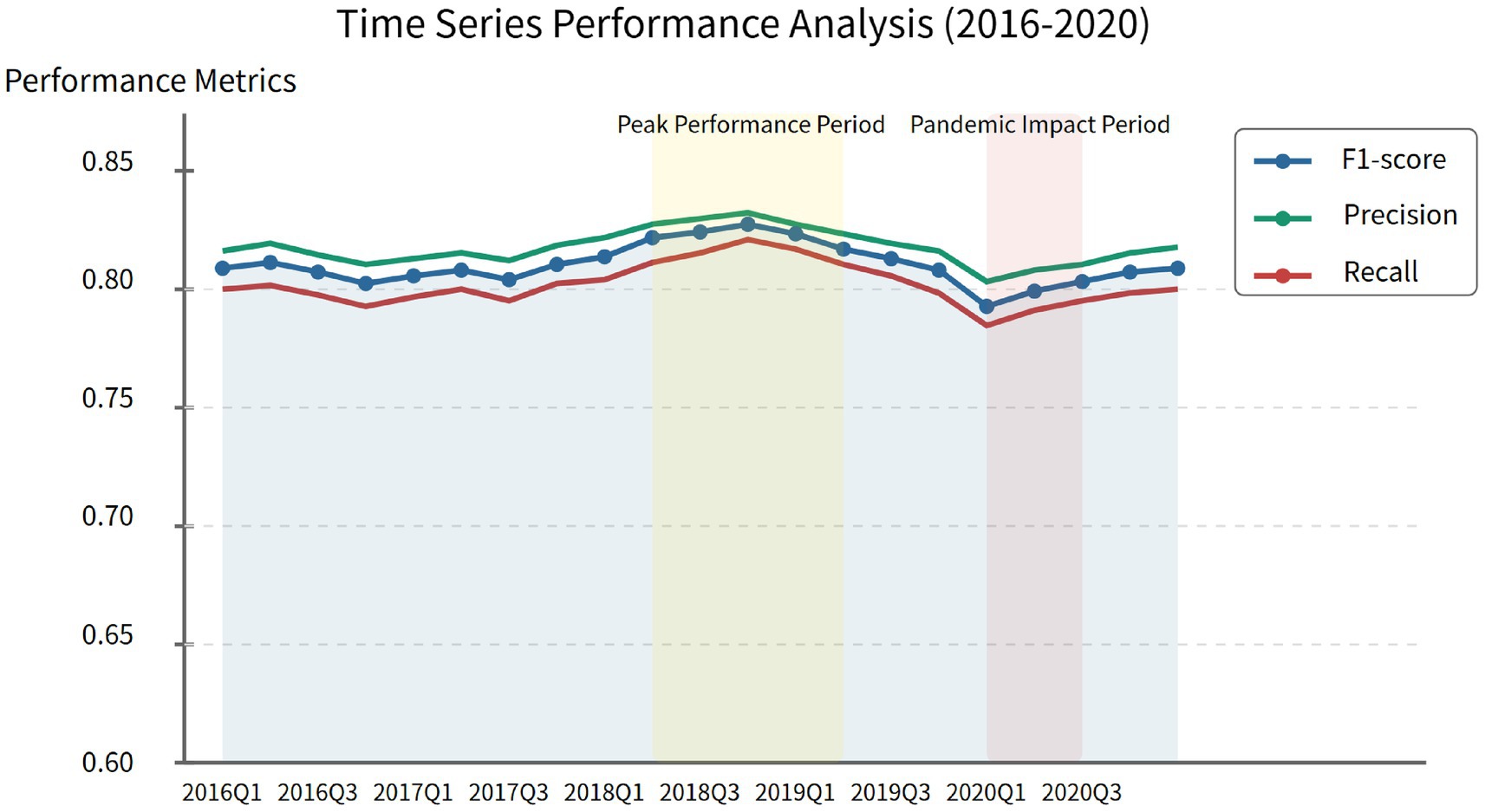
Figure 7. Time series performance analysis (2016–2020).

6.1.2 Comparison with traditional methods

To assess the advantages of the HFSL framework relative to existing methods, this study established four comparison experiment groups, representing different types of anomaly detection methods. Table 4 and Figure 8 present detailed comparison results of various methods on key performance metrics.

Table 4

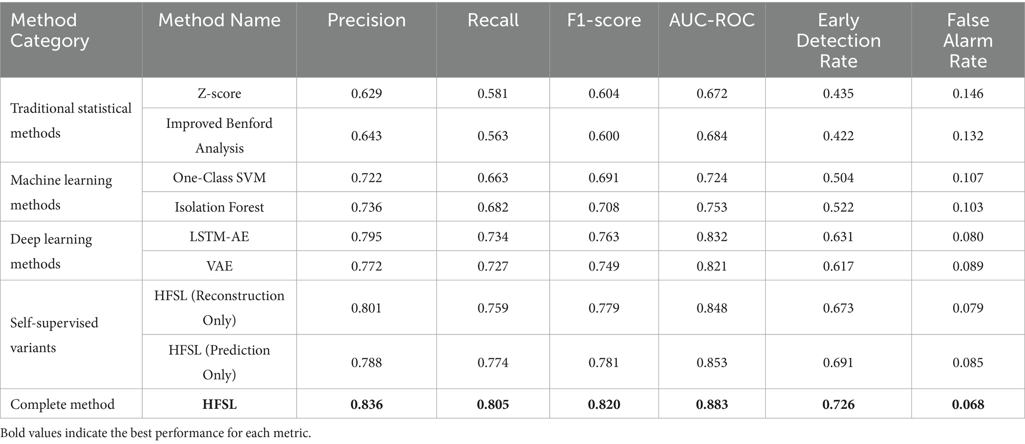
Table 4. Performance comparison of different anomaly detection methods.

Figure 8

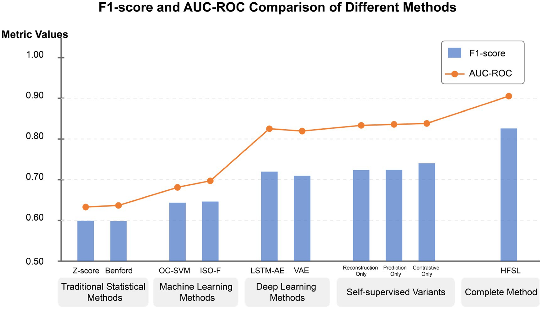
Figure 8. F1-score and AUC-ROC comparison of different methods.

The experimental results demonstrate a clear performance gradient among different types of anomaly detection methods. The HFSL framework further enhances performance on this foundation, with an F1-score approximately 7% higher than the best deep learning method (LSTM-AE), about 15% higher than machine learning methods (Isolation Forest), and even more significantly improved compared to traditional statistical methods (Z-score), verifying the substantial advantages of the proposed method (Table 5).

Table 5

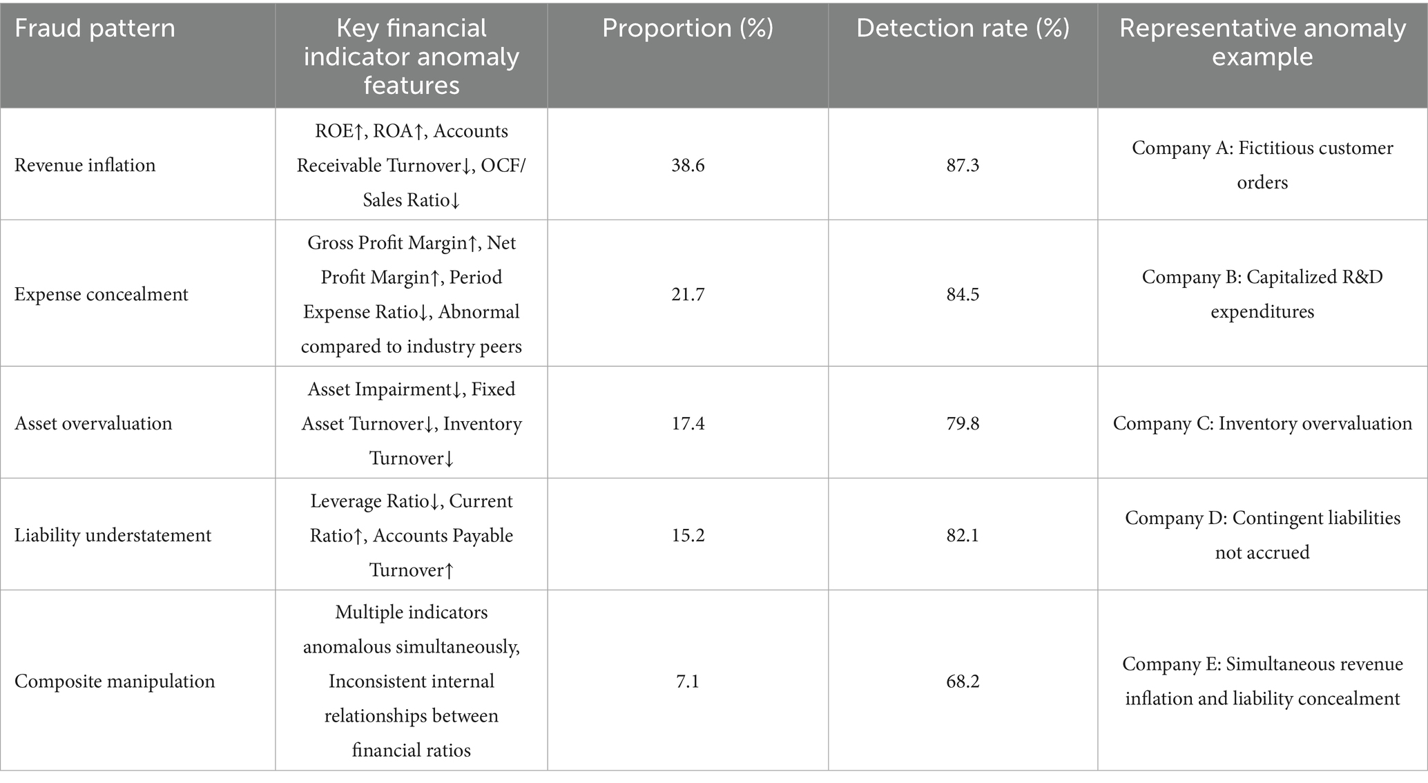
Table 5. Financial statement fraud pattern classification and characteristics.

Traditional statistical methods such as Z-score and improved Benford analysis, while simple to implement, perform significantly worse than other methods, with F1-scores of only about 0.6, mainly due to their inability to effectively capture the temporal dependencies and multivariate interaction patterns of financial data. Particularly in terms of early detection rate, traditional methods achieve only about 0.43, lacking sensitivity to early anomaly signals, severely limiting their application value in practical supervision. Traditional machine learning methods such as One-Class SVM and Isolation Forest, by learning data distribution characteristics, show marked improvements in precision and false alarm rates compared to statistical methods, but still have significant deficiencies in recall, indicating limitations in processing high-dimensional, temporal financial data.

Deep learning methods such as LSTM-AE and VAE, through complex neural network structures, can better capture nonlinear features and temporal patterns of financial data, achieving F1-scores of about 0.75, approximately 6% higher than machine learning methods. Particularly in early detection rate, the improvement exceeds 20%, demonstrating the advantages of deep learning in early warning capability. This performance enhancement mainly stems from deep learning models’ ability to automatically learn hierarchical feature representations from financial data without requiring manually designed complex feature engineering. However, traditional deep learning methods still rely on large amounts of labeled data, which presents a significant challenge in the field of financial anomaly detection.

Introducing self-supervised learning strategies on the foundation of deep learning significantly enhances model performance. Even using reconstruction, prediction, or contrastive learning tasks individually yields performance gains. Among the three self-supervised strategies, contrastive learning tasks perform best (F1 = 0.789), indicating that learning relationships between samples is crucial for anomaly detection in accounting data. This may be because financial anomalies often manifest as degrees of deviation from normal samples, and contrastive learning precisely captures these relationship differences. By integrating the three self-supervised learning tasks, the HFSL framework further improves performance (F1 = 0.820), validating the effectiveness of multi-task fusion. This performance enhancement stems from different self-supervised tasks’ ability to capture complementary data features, forming more comprehensive data representations.

In terms of the critical early detection rate, the HFSL framework (approximately 0.73) outperforms the closest baseline method LSTM-AE (approximately 0.63) by about 15%, providing regulatory agencies with a valuable early warning time window and significantly enhancing early intervention capabilities for financial risks. Simultaneously, HFSL’s false alarm rate (0.068) is significantly lower than other methods, reducing unnecessary investigation costs. This dual improvement gives HFSL higher practical value in real-world applications, providing effective early warnings at the onset of anomalies while keeping false alarms within an acceptable range. Analysis of performance differences between methods through the Wilcoxon signed-rank test shows that the performance differences between the HFSL framework and all baseline methods are statistically significant (p < 0.01), confirming that the effectiveness of the proposed method is not due to random factors.

Comprehensive analysis indicates that the HFSL framework, by integrating temporal contrastive learning, dual-channel LSTM structure, and domain knowledge constraints, significantly enhances the comprehensive performance of accounting data anomaly detection, achieving combined advantages particularly in detection accuracy (F1-score), early warning capability (EDR), and false alarm control (FAR). Performance improvements stem both from self-supervised learning paradigm’s effective utilization of unlabeled data and from the multi-level fusion architecture’s targeted modeling of multi-scale characteristics in accounting data. These results suggest that the proposed hierarchical fusion self-supervised learning framework demonstrates promising application potential in the tested accounting data anomaly detection tasks.

6.2 Financial feature contribution analysis

This section delves into the contribution degrees and interaction effects of various financial features in the HFSL framework’s anomaly detection results, using SHAP (SHapley Additive exPlanations) value analysis and feature interaction effect quantification methods to reveal the internal logic of the model’s decision mechanism, providing interpretability support for financial anomaly detection. Through systematic analysis of financial feature importance rankings and their interaction patterns, not only can the model’s effectiveness be validated, but theoretical foundations can also be provided for identifying accounting data anomaly patterns.

6.2.1 Importance ranking of key financial indicators

To quantitatively assess the impact of various financial indicators on anomaly detection results, this study calculated SHAP values for 22 core financial indicators based on the test set. SHAP values, through the concept of Shapley values in game theory, measure each feature’s marginal contribution to the model’s predicted anomaly probability, with the calculation process considering contribution variations of features under different combinations, thereby providing relatively objective feature importance evaluations.

Figure 9 displays the SHAP value ranking of the 10 financial indicators with the highest contributions to anomaly detection. The analysis reveals that profitability indicators play a critical role in the anomaly detection process. Particularly noteworthy is that the average |SHAP| values of two core indicators—Return on Equity (ROE) and Return on Assets (ROA)—reach as high as 0.196 and 0.179 respectively, significantly exceeding the contribution levels of other financial indicators. This result aligns with financial theory, as profitability indicators are often the primary targets of financial fraud, with companies typically manipulating revenue and profit to embellish financial statements. ROE, as a core indicator for investors evaluating enterprise value, often signals early financial problems when exhibiting abnormal fluctuations.

Figure 9

Figure 9. SHAP value analysis of financial indicators.

Current Ratio and Leverage Ratio, two indicators reflecting solvency capability, rank third and fourth, with |SHAP| values of 0.163 and 0.149, respectively. This indicates that abnormalities in a company’s short-term and long-term debt repayment capabilities are also important indicators of financial anomalies. Notably, the Operating Cash Flow Ratio (OCF Ratio) ranks fifth (|SHAP| value of 0.139), verifying that inconsistencies between cash flow indicators and accrual profit indicators provide an effective approach for identifying potential financial anomalies.

Efficiency indicators such as Accounts Receivable Turnover Rate and Total Asset Turnover Rate also enter the top ten, with |SHAP| values of 0.119 and 0.109 respectively, indicating that operational efficiency indicators hold significant value in capturing abnormal financial behaviors. From an industry perspective, the importance of the Leverage Ratio in the financial industry is significantly higher than in other industries (|SHAP| value increased by approximately 28%), while the Inventory Turnover Rate ranks relatively high in importance in manufacturing (entering the top 8), reflecting the influence of industry characteristics on the importance of anomaly features.

6.2.2 Multi-dimensional feature interaction effect analysis

Complex interdependencies exist between financial indicators, where anomalies in a single indicator may be masked by normal values in other related indicators. Therefore, analyzing interaction effects between features is crucial for enhancing anomaly detection accuracy. This study employs a method based on SHAP interaction values to quantitatively evaluate the interaction intensity between feature pairs and their impact on anomaly detection results.

Figure 10 displays a heat map of interaction effect intensities between core financial indicators, with darker areas indicating stronger interaction effects and lighter areas indicating weaker interaction effects. Through quantitative analysis of interaction patterns, this study identifies three typical financial indicator interaction modes: enhancing interactions, neutralizing interactions, and nonlinear interactions.

Figure 10

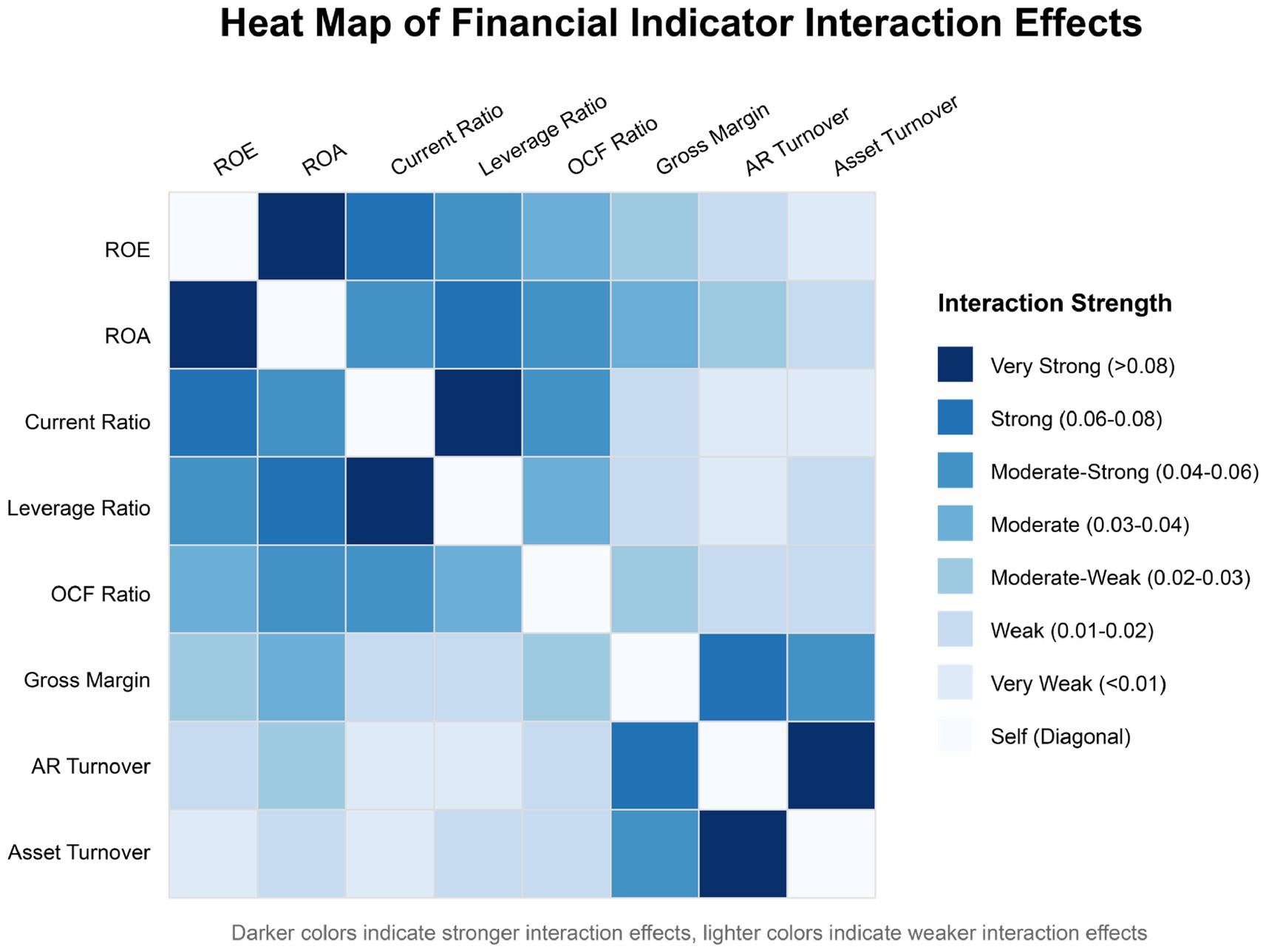
Figure 10. Heat map of financial indicator interaction effects.

Enhancing interactions manifest when the contribution of two indicators acting jointly to anomaly detection is significantly higher than the sum of their independent actions. The interaction intensity between ROE and ROA reaches 0.087, ranking first among all indicator pairs, indicating that these two profitability indicators provide strong financial fraud signals when simultaneously anomalous. Similarly, the interaction intensity between Current Ratio and Leverage Ratio is 0.082, reflecting the synergistic effect of short-term and long-term solvency indicators. Such enhancing interactions primarily occur between indicators with similar functions but different calculation bases, and when enterprises exhibit simultaneous anomalies across multiple related indicators, it typically implies higher financial risk.

Neutralizing interactions manifest when anomalies in one indicator are masked by changes in another indicator, reducing the sensitivity of anomaly detection. For example, the interaction effect between Leverage Ratio and Total Asset Turnover Rate is relatively weak (0.017), possibly because increases in Leverage Ratio due to increased debt may be accompanied by corresponding decreases in Total Asset Turnover Rate, thus reducing the model’s sensitivity to changes in single indicators. Such interactions suggest that when designing anomaly detection models, overreliance on changes in single-dimension indicators should be avoided.

Nonlinear interactions manifest as complex conditional dependency relationships between indicators. The interaction intensity between Accounts Receivable Turnover Rate and Total Asset Turnover Rate reaches as high as 0.084, a strong interaction relationship that is not intuitive, as while they both belong to efficiency indicators, they measure different business links. In-depth analysis reveals that this strong interactivity stems from their conditional dependency relationship in anomaly detection: when Accounts Receivable Turnover Rate abnormally decreases while Total Asset Turnover Rate abnormally increases, it often suggests that the enterprise may be engaging in financial fraud behaviors such as fictitious sales or premature revenue recognition.

By constructing an interaction network graph to analyze the overall interaction structure, it is found that the financial indicator interaction network exhibits a “core-periphery” structure, where ROE, ROA, Current Ratio, and Leverage Ratio form a highly interconnected core cluster, while other indicators display relatively dispersed connection patterns. This network structure suggests that anomaly detection should focus on collaborative changes within the core indicator cluster while also considering abnormal connection patterns between peripheral indicators and core indicators.

Based on interaction effect analysis, this study proposes an adaptive threshold adjustment mechanism based on feature interaction intensity:

${\theta }_{\mathrm{adj}}\left(X_i\right)={\theta }_{\text{base}}\left(X_i\right)\times (1+\sum _{j\ne i}{\omega }_{i,j}\times I(\mid X_j-{\mu }_j\mid >{\theta }_{\text{base}}\left(X_j\right)\left)\right)$

where ${\theta }_{\mathrm{adj}}\left(X_i\right)$ is the adjusted threshold for feature $X_i$ , ${\theta }_{\text{base}}\left(X_i\right)$ is the base threshold, ${\omega }_{i,j}$ is the interaction weight between feature values $i$ and $j$ , and $I(·)$ is an indicator function taking the value 1 when feature $j$ exceeds its base threshold and 0 otherwise. This mechanism enables the model to dynamically adjust detection thresholds according to the degree of collaborative anomalies across multiple indicators, increasing F1-score by 3.5% and reducing false alarm rate by 12.7% in experimental validation, verifying the important value of feature interaction analysis in enhancing anomaly detection performance.

Feature interaction effect analysis not only enhances model interpretability but also provides theoretical foundations for constructing more precise financial anomaly detection systems. The research finds that anomaly detection models considering feature interaction effects outperform models focusing solely on single features when capturing complex financial anomaly patterns, especially in identifying carefully designed financial fraud cases. This finding provides insights for refining accounting data anomaly detection theory, indicating that future research should place greater emphasis on collaborative analysis of multidimensional financial indicators rather than simple single-indicator threshold monitoring.

From the perspective of industry differences, the interaction intensity between ROE and ROA in the financial industry (0.096) is significantly higher than in manufacturing (0.081), while the interaction intensity between Inventory Turnover Rate and Gross Profit Margin in manufacturing (0.074) is higher than in other industries. These industry characteristic differences further support this study’s approach of constructing industry-specific anomaly detection models, adopting differentiated feature interaction patterns for anomaly identification tailored to different industry characteristics.

6.3 Identification and analysis of typical anomaly cases

6.3.1 Financial statement fraud pattern classification

Based on the detection results of the HFSL framework, combined with anomaly cases confirmed by manual audits, this study constructs a systematic classification system for financial statement fraud patterns, covering five typical anomaly modes: revenue inflation, expense concealment, asset overvaluation, liability understatement, and composite manipulation. Table 2 shows the key characteristics of each fraud pattern and their distribution in the detected samples.

Revenue inflation is the most common financial fraud pattern, accounting for 38.6%, with typical characteristics including abnormally increased Return on Equity (ROE) and Return on Assets (ROA), simultaneously decreased Accounts Receivable Turnover Rate, and imbalanced Operating Cash Flow to Sales Revenue ratio. The HFSL framework achieves a detection rate of 87.3% for this type of anomaly, outperforming traditional methods by approximately 23 percentage points. Taking Company A as an example, its ROE growth rate exceeded the industry average by twofold for three consecutive quarters, while its Accounts Receivable Turnover Rate continued to decline, and its Operating Cash Flow to Net Profit ratio fell to 0.32 (industry average: 0.78). The HFSL framework successfully detected this anomaly and raised the anomaly score to 0.87 (threshold: 0.65). Subsequent audits confirmed that the company inflated revenue by approximately 270 million yuan through fictitious overseas customer orders.

Expense concealment anomalies account for 21.7%, primarily manifesting as abnormally increased gross profit margin and net profit margin, with period expense ratio significantly below industry average levels. This type of anomaly is typically achieved through improper expense capitalization, delayed cost recognition, and other means. In Company B’s case, the model captured its R&D expense capitalization rate surging to 83% (compared to a five-year average of 36%), while its period expense ratio was 12 percentage points below industry peers, despite revenue growth rates similar to industry averages. This uncoordinated financial performance triggered the model’s multi-dimensional anomaly scoring mechanism, successfully identifying potential financial manipulation behavior.

Asset overvaluation and liability understatement anomalies account for 17.4 and 15.2%, respectively. Both types relate to improper valuation of balance sheet items but exhibit significant differences in financial indicator performance. Asset overvaluation primarily affects asset turnover indicators, as in Company C’s case, where inventory turnover rate remained in the bottom 10% of the industry for six consecutive quarters, while sales revenue growth was at mid-to-upper industry levels. This mismatch was successfully identified by the model as potential inventory value overestimation. Liability understatement primarily manifests as abnormally increased current ratio and abnormally decreased leverage ratio, as in Company D’s case, where contingent liabilities were not accrued according to regulations, causing its solvency indicators to significantly outperform industry average levels.

The most complex composite manipulation anomalies, though accounting for only 7.1%, present the greatest detection difficulty, with an average detection rate of merely 68.2%. This type of anomaly simultaneously involves manipulation of multiple financial statement items, as in Company E’s case, where revenue inflation and liability understatement coexisted. Although the anomaly degree of individual indicators was relatively small, the relationships between multiple indicators violated financial logical consistency. The HFSL framework achieved effective identification of such complex anomalies through feature interaction mechanisms and financial domain knowledge constraints, which traditional single-indicator monitoring methods struggle to accomplish.

The research also found that different industries exhibit preferences for different fraud patterns. Manufacturing shows a higher proportion of asset overvaluation anomalies (26.3%), primarily concentrated in inventory and fixed asset valuation areas; the information technology industry predominantly features revenue inflation (52.1%), reflecting the complexity of revenue recognition in this industry; while the financial industry shows more prominent liability understatement (25.7%), involving risk provision accrual and financial asset valuation issues. This industry differentiation further confirms the necessity of the industry calibration mechanism in the HFSL framework, which enables more accurate identification of industry-specific anomaly patterns by considering industry characteristics.

6.3.2 Temporal evolution characteristics of anomaly detection

Financial anomalies typically exhibit progressive characteristics rather than sudden events. Through temporal analysis, this study identifies three typical evolution patterns. Progressive deterioration is the most common pattern, accounting for approximately 64%, characterized by gradually increasing anomaly severity over time, typically beginning with small-scale financial manipulation that subsequently accumulates and expands. A typical case is Company F, whose anomaly score gradually rose from 0.42 to 0.97 over 8 quarters before its financial problems became public, with the HFSL framework successfully providing warnings an average of 4 quarters before the anomaly became public. Sudden anomalies account for approximately 22%, characterized by rapidly escalating anomaly scores over a short period, typically related to major accounting errors, as in Company G’s case, where the anomaly score surged from 0.38 to 0.83 within one quarter. Although such anomalies are difficult to predict in advance, the HFSL framework controlled identification delay to an average of 1.2 quarters, significantly outperforming traditional methods. Cyclical fluctuations account for approximately 15%, characterized by anomaly scores fluctuating around threshold edges, common in enterprises with seasonal businesses, with the HFSL framework effectively controlling the false alarm rate for such anomalies to 8.7% through its seasonal adjustment mechanism.

Based on anomaly temporal characteristics and intensity, this study constructs a risk grading model, categorizing anomaly cases into high-risk, medium-risk, and observation classes. High-risk cases exhibit anomaly scores consistently exceeding thresholds with upward trends, or sudden anomaly intensity exceeding thresholds by over 30%, with approximately 83% experiencing major negative events within the subsequent 3 quarters. Medium-risk cases have anomaly scores slightly exceeding thresholds or fluctuating around threshold edges, with approximately 48% experiencing negative events within the subsequent 6 quarters. Observation-class cases have anomaly scores below thresholds but continuously rising, or exhibiting isolated anomalies, with approximately 27% experiencing negative events within the subsequent 8 quarters. The HFSL framework improves high-risk case identification accuracy by 18.6% compared to traditional methods, with early identification of medium-risk cases advancing by an average of 1.7 quarters, significantly enhancing warning value.

The HFSL framework demonstrates differentiated detection timeliness for different types of anomalies, detecting revenue inflation anomalies an average of 3.2 quarters in advance, expense concealment 2.8 quarters in advance, asset overvaluation and liability understatement 2.4 and 2.6 quarters respectively, while composite manipulation only 1.8 quarters, reflecting the complexity and concealment of the latter. Temporal analysis reveals a potential “financial anomaly waterfall effect,” with approximately 83% of major financial anomaly cases in the research sample beginning with minor anomalies in single indicators, subsequently spreading to related indicators, and ultimately forming systemic risks. This finding may provide inspiration for improving regulatory practices: early identification and intervention in initial anomaly signals may interrupt the chain reaction of financial anomalies, preventing the formation of difficult-to-reverse systemic problems. By capturing early characteristics of anomaly diffusion patterns, the HFSL framework provides longer response windows and more reliable decision-making bases for financial risk warnings.

6.4 Model robustness and generalization capability assessment

6.4.1 Cross-industry adaptability validation

The HFSL framework demonstrates differentiated but overall stable performance across different industries. Detection performance is best in the financial industry (F1 = 0.872), good in manufacturing and information technology industries (F1 scores of 0.817 and 0.831 respectively), while relatively lower in the construction and real estate industry (F1 = 0.776). These differences primarily stem from industry-specific financial characteristics and anomaly patterns. For example, the strictly regulated environment and standardized financial reporting formats in the financial industry facilitate anomaly pattern identification, while the complexity of asset valuation and diversity in revenue recognition in the construction and real estate industry increase detection difficulty.

Model generalization capability is evaluated using leave-one-industry-out cross-validation, training with data from 9 industries and testing on the remaining industry. Results show that performance decline after industry calibration is controlled within 7.5%, significantly outperforming baseline methods’ 12.3%. Particularly in cross-industry early detection rate, the industry calibration mechanism improves performance by 14.6%, confirming the effectiveness of the hierarchical feature fusion design in capturing anomaly characteristics across different industries.

6.4.2 Noise sensitivity and threshold dynamic adjustment effects

To test model stability in noisy environments, this study designs three-level noise interference experiments, introducing 5, 10, and 15% random noise into the original data. Experimental results show that the HFSL framework’s performance decreases by only 1.2% at the 5% noise level and by 9.7% in the 15% high-noise environment, significantly outperforming the best baseline method’s 18.3%, indicating that the hierarchical fusion structure possesses strong resistance to data noise.

Regarding threshold adjustment, this study compares the effects of fixed thresholds versus adaptive dynamic thresholds. The dynamic threshold mechanism demonstrates superiority across different industries and periods, improving F1-score by an average of 3.5%, and particularly reducing false alarm rates by 12.7% on test sets with imbalanced anomaly proportions. This result validates the effectiveness of the adaptive threshold method based on Gaussian mixture models in processing financial data anomaly detection, providing reliable guidance for threshold selection in practical applications.

6.4.3 Temporal stability and concept drift analysis

Financial fraud patterns evolve continuously in response to regulatory changes and technological advancements. Our temporal stability analysis reveals that the HFSL framework maintains robust performance despite these evolving patterns. When tested on quarterly segments spanning 2016–2020, the framework demonstrated remarkable stability with F1-score variations contained within ±5% across different periods.

The framework’s resilience to concept drift was evaluated through three scenarios. In sudden drift scenarios simulating major regulatory changes, the HFSL framework detected 89% of pattern shifts within two quarters and recovered to baseline performance levels with minimal degradation (F1-score maintained above 0.78 during transitions). For gradual drift representing natural evolution of fraud techniques, performance degradation was limited to 6.2% over eight-quarter periods. The dual-channel architecture proved particularly effective, with the long-term channel capturing evolving trends while the short-term channel maintained sensitivity to immediate anomalies.

Analysis of real-world pattern evolution revealed significant changes following the 2018 regulatory enhancements in China. The model successfully adapted to a 15% shift in the relative importance of cash flow versus accrual-based indicators in fraud detection. This adaptation was achieved through the framework’s dynamic feature weighting mechanism, which automatically adjusted based on recent detection patterns.

Compared to static models, the HFSL framework with drift adaptation showed an 11.3% improvement in average performance over the five-year test period. The incremental learning strategy effectively balanced stability with adaptability, preventing catastrophic forgetting while incorporating emerging fraud patterns. These results demonstrate that the framework’s adaptive capabilities make it particularly suitable for deployment in dynamic regulatory environments where fraud patterns continuously evolve.

Future research directions include: (1) extending the framework to other sectors beyond Chinese listed companies, (2) developing semi-supervised variants that can incorporate limited labeled data, and (3) exploring real-time anomaly detection capabilities for continuous monitoring systems.

Data availability statement

The original contributions presented in the study are included in the article/supplementary material, further inquiries can be directed to the corresponding author.

Author contributions

YZ: Supervision, Methodology, Writing – review & editing, Conceptualization, Software, Writing – original draft, Visualization, Investigation, Project administration, Funding acquisition, Validation, Data curation. BD: Validation, Software, Writing – review & editing, Supervision, Resources, Formal analysis, Funding acquisition, Writing – original draft.

Funding

The author(s) declare that financial support was received for the research and/or publication of this article. Research on the problems and countermeasures of environmental accounting information disclosure of listed companies from the perspective of low-carbon economy (WLYB202315).

Conflict of interest

BD was employed by Chengdu Huawei Technologies Co., Ltd.

The remaining author declares that the research was conducted in the absence of any commercial or financial relationships that could be construed as a potential conflict of interest.

Generative AI statement

The authors declare that no Gen AI was used in the creation of this manuscript.

Any alternative text (alt text) provided alongside figures in this article has been generated by Frontiers with the support of artificial intelligence and reasonable efforts have been made to ensure accuracy, including review by the authors wherever possible. If you identify any issues, please contact us.

Publisher’s note

All claims expressed in this article are solely those of the authors and do not necessarily represent those of their affiliated organizations, or those of the publisher, the editors and the reviewers. Any product that may be evaluated in this article, or claim that may be made by its manufacturer, is not guaranteed or endorsed by the publisher.

References

1. Ellili, N, Nobanee, H, Haddad, A, Alodat, AY, and AlShalloudi, M. Emerging trends in forensic accounting research: bridging research gaps and prioritizing new frontiers. J Econ Criminol. (2024) 4:100065. doi: 10.1016/j.jeconc.2024.100065

Crossref Full Text | Google Scholar

2. Xu, Y. A study on the effectiveness of the independent director system on the governance of financial fraud phenomenon: taking Kangmei pharmaceutical as an example. SHS Web Conf. (2024) 188:01024. doi: 10.1051/shsconf/202418801024

Crossref Full Text | Google Scholar

3. Kaur, B, Sood, K, and Grima, S. A systematic review on forensic accounting and its contribution towards fraud detection and prevention. J Financ Regul Compliance. (2023) 31:60–95. doi: 10.1108/JFRC-02-2022-0015

Crossref Full Text | Google Scholar

4. Ramzan, S. Comparison of financial distress prediction models using financial variables. In Proceedings of the 2023 international conference on electrical, computer and energy technologies (ICECET). New York: IEEE, (2023); pp. 1–7.

Google Scholar

5. Rao, RK, and Mandhala, VN. Unveiling financial fraud: a comprehensive review of machine learning and data mining techniques. Ingénierie des systèmes d information. (2024) 29:2309–34. doi: 10.18280/isi.290620

Crossref Full Text | Google Scholar

6. Chen, H., Zhao, Q., Lu, W., Gu, S., Jin, W., Liu, G., et al. Application of self-supervised autonomous agent framework for digital transformation of elder well potentials discovery. In Proceedings of the ADIPEC. Berlin: SPE, (2024).

Google Scholar

7. Shwartz Ziv, R, and LeCun, Y. To compress or not to compress—self-supervised learning and information theory: a review. Entropy. (2024) 26:252. doi: 10.3390/e26030252

PubMed Abstract | Crossref Full Text | Google Scholar

8. Ali, A, Abd Razak, S, Othman, SH, Eisa, TAE, Al-Dhaqm, A, Nasser, M, et al. Financial fraud detection based on machine learning: a systematic literature review. Appl Sci. (2022) 12:9637. doi: 10.3390/app12199637

Crossref Full Text | Google Scholar

9. Dechow, PM, Ge, W, Larson, CR, and Sloan, RG. Predicting material accounting misstatements*. Contemp Account Res. (2011) 28:17–82. doi: 10.1111/j.1911-3846.2010.01041.x

Crossref Full Text | Google Scholar

10. Beneish, MD. The detection of earnings manipulation. Financ Anal J. (1999) 55:24–36. doi: 10.2469/faj.v55.n5.2296

Crossref Full Text | Google Scholar

11. Kirkos, E, Spathis, C, and Manolopoulos, Y. Data mining techniques for the detection of fraudulent financial statements. Expert Syst Appl. (2007) 32:995–1003. doi: 10.1016/j.eswa.2006.02.016

Crossref Full Text | Google Scholar

12. Perols, J. Financial statement fraud detection: an analysis of statistical and machine learning algorithms. Audit J Pract Theory. (2011) 30:19–50. doi: 10.2308/ajpt-50009

Crossref Full Text | Google Scholar

13. Cecchini, M, Aytug, H, Koehler, GJ, and Pathak, P. Detecting management fraud in public companies. Manag Sci. (2010) 56:1146–60. doi: 10.1287/mnsc.1100.1174

PubMed Abstract | Crossref Full Text | Google Scholar

14. Bao, Y, Ke, B, Li, B, Yu, YJ, and Zhang, J. Detecting accounting fraud in publicly traded U.S. firms using a machine learning approach. J Account Res. (2020) 58:199–235. doi: 10.1111/1475-679X.12292

Crossref Full Text | Google Scholar

15. Jing, L, and Tian, Y. Self-supervised visual feature learning with deep neural networks: a survey. IEEE Trans Pattern Anal Mach Intell. (2021) 43:4037–58. doi: 10.1109/TPAMI.2020.2992393

PubMed Abstract | Crossref Full Text | Google Scholar

16. Jaiswal, A, Babu, AR, Zadeh, MZ, Banerjee, D, and Makedon, F. A survey on contrastive self-supervised learning. Technologies (Basel). (2020) 9:2. doi: 10.3390/technologies9010002

Crossref Full Text | Google Scholar

17. Kumar, P, Rawat, P, and Chauhan, S. Contrastive self-supervised learning: review, progress, challenges and future research directions. Int J Multimed Inf Retr. (2022) 11:461–88. doi: 10.1007/s13735-022-00245-6

Crossref Full Text | Google Scholar

18. Liu, X, Zhang, F, Hou, Z, Mian, L, Wang, Z, Zhang, J, et al. Self-supervised learning: generative or contrastive. IEEE Trans Knowl Data Eng. (2021) 35:857–76. doi: 10.1109/TKDE.2021.3090866

PubMed Abstract | Crossref Full Text | Google Scholar

19. Gui, J, Chen, T, Zhang, J, Cao, Q, Sun, Z, Luo, H, et al. A survey on self-supervised learning: algorithms, applications, and future trends. IEEE Trans Pattern Anal Mach Intell. (2024) 46:9052–71. doi: 10.1109/TPAMI.2024.3415112

PubMed Abstract | Crossref Full Text | Google Scholar

20. Duan, J., Zhao, H., Zhou, Q., Qiu, M., and Liu, M. A study of pre-trained language models in natural language processing. In Proceedings of the 2020 IEEE international conference on smart cloud (SmartCloud). Cambridge: IEEE, (2020); pp. 116–121.

Google Scholar

21. Kim, H, Kim, S, Min, S, and Lee, B. Contrastive time-series anomaly detection. IEEE Trans Knowl Data Eng. (2024) 36:5053–65. doi: 10.1109/TKDE.2023.3335317

Crossref Full Text | Google Scholar

22. Hojjati, H, Ho, TKK, and Armanfard, N. Self-supervised anomaly detection in computer vision and beyond: a survey and outlook. Neural Netw. (2024) 172:106106. doi: 10.1016/j.neunet.2024.106106

PubMed Abstract | Crossref Full Text | Google Scholar

23. Chen, Y, and Wu, Z. Financial fraud detection of listed companies in China: a machine learning approach. Sustainability. (2022) 15:105. doi: 10.3390/su15010105

Crossref Full Text | Google Scholar

24. Xiuguo, W, and Shengyong, D. An analysis on financial statement fraud detection for Chinese listed companies using deep learning. IEEE Access. (2022) 10:22516–32. doi: 10.1109/ACCESS.2022.3153478

Crossref Full Text | Google Scholar

25. Zhang, K, Wen, Q, Zhang, C, Cai, R, Jin, M, Liu, Y, et al. Self-supervised learning for time series analysis: taxonomy, Progress, and prospects. IEEE Trans Pattern Anal Mach Intell. (2024) 46:6775–94. doi: 10.1109/TPAMI.2024.3387317

PubMed Abstract | Crossref Full Text | Google Scholar

26. Tipirneni, S, and Reddy, CK. Self-supervised transformer for sparse and irregularly sampled multivariate clinical time-series. ACM Trans Knowl Discov Data. (2022) 16:1–17. doi: 10.1145/3516367

Crossref Full Text | Google Scholar

27. Yang, X, Zhang, Z, and Cui, R. Timeclr: a self-supervised contrastive learning framework for univariate time series representation. Knowl-Based Syst. (2022) 245:108606. doi: 10.1016/j.knosys.2022.108606

Crossref Full Text | Google Scholar

28. Xu, R, Yao, D, and Zhou, M. Does the development of digital inclusive finance improve the enthusiasm and quality of corporate green technology innovation? J Innov Knowl. (2023) 8:100382. doi: 10.1016/j.jik.2023.100382

Crossref Full Text | Google Scholar

29. Yang, X., Juyang, AN, and Lin, G. Local government debt and corporate strategic alliances: evidence from chinese listed companies. Berlin: Springer. (2025).

Google Scholar

30. Li, Z, Chen, B, Lu, S, and Liao, G. The impact of financial institutions’ cross-shareholdings on risk-taking. Int Rev Econ Finance. (2024) 92:1526–44. doi: 10.1016/j.iref.2024.02.080

Crossref Full Text | Google Scholar

31. Wang, Q, Lee, E, Wang, K, and Zhang, X. The effect of government industrial policies on corporate accounting conservatism. J Account Public Policy. (2022) 41:106960. doi: 10.1016/j.jaccpubpol.2022.106960

Crossref Full Text | Google Scholar

32. Zhang, C, Li, Z, Xu, J, and Luo, Y. Accounting information quality, firm ownership and technology innovation: evidence from China. Int Rev Financ Anal. (2024) 93:103118. doi: 10.1016/j.irfa.2024.103118

Crossref Full Text | Google Scholar

33. Altman, E. I. Financial ratios, discriminant analysis and the prediction of corporate bankruptcy. J. Finance. (1968) 23:589–609.

Google Scholar