A mathematical model for data-driven synthesis of neuron morphologies based on random walks

Recent advances in computational resources have enabled the development of large-scale, biophysically detailed brain models, which require numerous three-dimensional neuron morphologies exhibiting realistic cell-to-cell variability. However, the limited availability of experimental reconstructions restricts parameter estimation for many morphology synthesis algorithms, which typically rely on extensive datasets. Here, we propose enhancing our branching-and-annihilating random walk method by incorporating a set of mathematical equations that estimate branching and annihilation probabilities directly from Sholl plots and branch point counts. Because these morphological metrics are commonly reported in the literature, our approach facilitates the generation of realistic three-dimensional morphologies even in the absence of experimental reconstructions.

1 Introduction

Recent advances in computational resources have promoted the development of large-scale biophysically-detailed models of the brain [1–4], which require numerous three-dimensional neuron morphologies with realistic levels of cell-to-cell variability. Theoretical and experimental studies demonstrated that the geometric characteristics of neuronal morphologies influence their electrotonic and integrative properties [5–9], with direct functional implications for the dynamics of brain regions [1, 3, 10–13]. Furthermore, experimental evidence confirmed that cell-to-cell variability is not merely the result of biological randomness but contributes to the robustness and adaptability of neural circuits [14, 15]. Taken together, these findings underscore the importance of reproducing these aspects in biophysically-detailed reconstructions to simulate neural dynamics with high realism.

Due to the limited availability of experimental reconstructions, various algorithms have been developed to synthesize neuronal morphologies that capture the characteristics of their biological counterparts [1, 16–18]. For example, we designed a method based on branching-and-annihilating random walks to generate three-dimensional morphologies of olfactory mitral and tufted cells that were indistinguishable from their biological counterparts and exhibited experimentally observed levels of cell-to-cell variability [1, 3]. However, these methods still require many experimental reconstructions to determine the parameter values, which poses a major challenge when such data are scarce. Furthermore, these methods still retain a high degree of empiricism and rely on extensive parameter tuning, while rigorous mathematical characterization remains lacking.

Alternatively, we propose a mathematical characterization of our previous method [1, 3], describing the influence of branching and annihilation probabilities on Sholl plots and branch point counts. We have shown how these equations can be linked to experimental estimates of such metrics, allowing for the direct calculation of both probabilities. Therefore, this preliminary result provides a rigorous mathematical foundation that will strengthen our earlier method, reducing its reliance on empirical parameter tuning.

2 Materials and methods

2.1 Software details

The model was validated through simulations implemented in Python 3. Parameters were estimated by fitting using quadratic programming with the Pyomo package. NumPy and Pandas were employed for data handling, while SciPy was used for statistical tests. Data visualization was performed with Matplotlib.

2.2 Code availability

The source code is publicly available on GitHub, in the repository NeuronSynthesis.

2.3 Morphological inspection

The model was tested on Sholl plots and branch point counts obtained from experimentally reconstructed three-dimensional neuron morphologies, using a custom Python script. For each neuron type, the method was applied to the subtree (apical or basal) representing the most morphologically complex component. All morphologies are publicly available at NeuroMorpho.Org [19].

2.3.1 Semilunar and pyramidal neurons from the piriform cortex

We considered three-dimensional reconstructions of semilunar (SL) (n = 3) and pyramidal (PYR) (n = 16) neurons from the piriform cortex of rats [6], focusing on their apical dendritic trees. Following visual inspection, we discarded four PYR morphologies due to apparent damage or deformation in their dendritic arbors, to avoid biasing the experimental measurements considered in this study.

2.3.2 Tufted and mitral cells from the olfactory bulb

We considered three-dimensional reconstructions of tufted (TF) (n = 5) and mitral (MC) (n = 9) cells from the main olfactory bulb of mice [20], focusing on their basal dendritic trees. During visual inspection, we identified apical dendrites that had been erroneously labeled as basal in several morphologies, which were discarded from our analysis (TF: n = 5; MC: n = 1). The tests conducted on these cells are shown in Supplementary Figure S1.

2.3.3 Neocortical pyramidal neurons

We considered three-dimensional reconstructions from Markrams dataset [2], which includes neocortical pyramidal neurons from different cortical layers (n = 84). Following the classification described in the original study, we selected only “late-bifurcating pyramidal neurons” with somata located in layer VI, and retained only those reconstructions that did not show truncated or deformed apical trees (n = 9). For subsequent analyses, we focused on their apical dendritic trees. The tests conducted on these cells are shown in Supplementary Figure S2.

2.4 Statistical analysis

For all tests, statistical significance was defined as p < 0.01 (without Bonferroni adjustment). To compare simulation and experimental data, we used two-sample, two-sided bootstrap methods for mean and variance comparison, respectively, based on the description provided by Davison and Hinkley [21] (see Figure 3). A Bonferroni correction was applied when comparing simulated and experimental Sholl plots (see Figures 3A, B). To compare simulation and theoretical values, we used a one-sample, two-sided bootstrap methods for mean and variance comparisons, respectively. To compare the number of branch points obtained with different configurations of parameters, we used a one-sample, two-sided t-test and a χ² test for mean and variance comparisons, respectively (see Figure 1C).

Figure 1

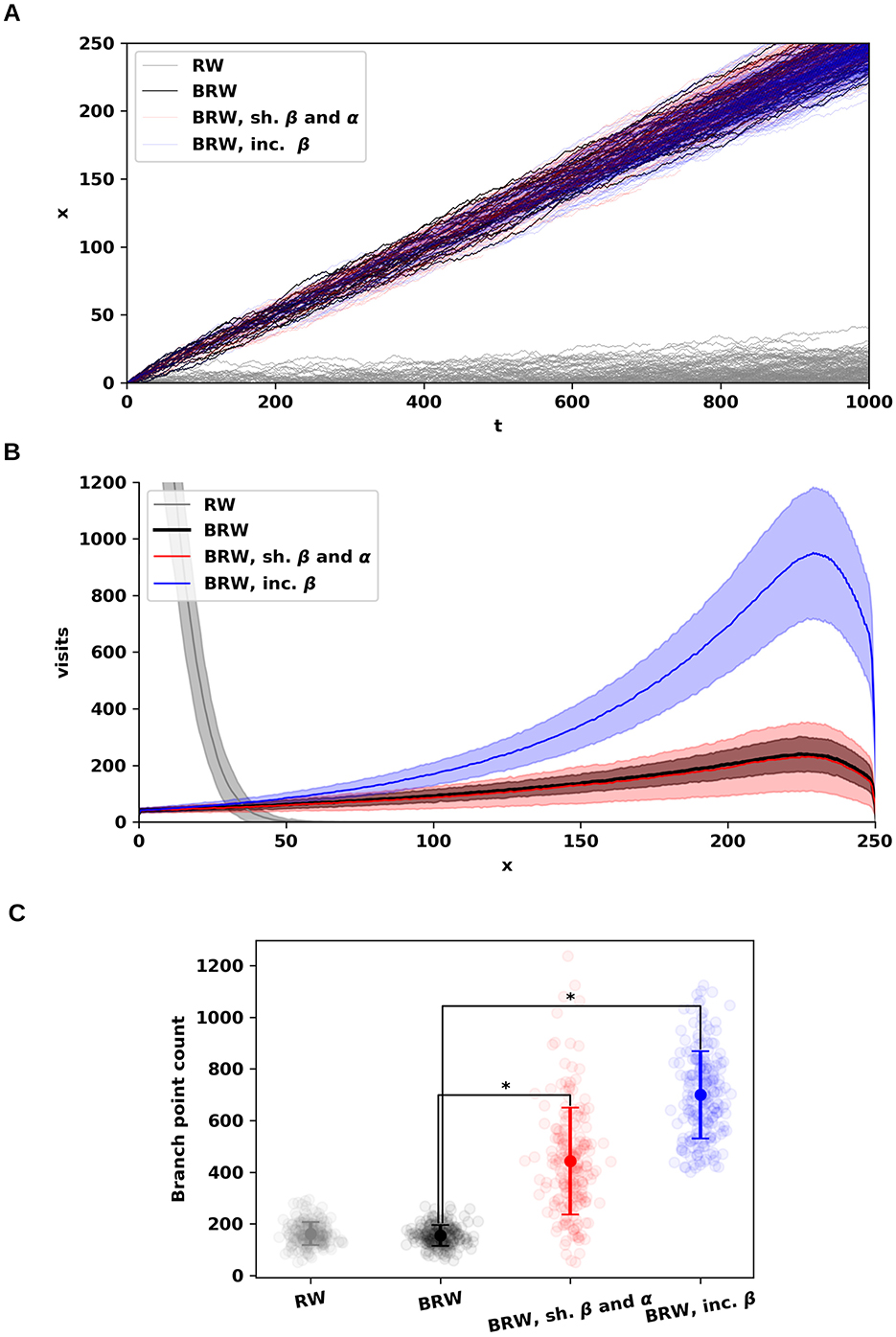
Figure 1. Random walks under varying levels of somatofugal bias and branching–annihilating dynamics. (A) Distance from the origin over time for four random walk conditions: unbiased (gray; r = 0.5, β = 0.005, α = 0.001); somatofugal bias (black; r = 0.75, β = 0.005, α = 0.001), which increased net distance from the origin; increased branching and annihilation rates (red; r = 0.75, β = 0.015, α = 0.011); and increased branching rate only (blue; r = 0.75, β = 0.035, α = 0.001). The spatial step size was held the same for all configurations (Δx = 0.5). For each parameter combination, the estimate is based on multiple independent trials (n = 200). (B) Distribution of visit counts as a function of distance from the origin for the same configurations shown in (A), averaged across trials. Combined increase in branching and annihilation rates increased variance without affecting the mean number of visits (black vs. red), while increasing branching rate alone raised both mean and variance (black vs. blue). (C) Total number of branch points under each condition shown in (B). An increase in branching and/or annihilation rates led to higher mean and variance of branch point counts (mean ± SD): RW (gray): 162.2 ± 44.7 (±SD); BRW (black): 155.7 ± 40.1; BRW with increased β and α (red): 443.1 ± 205.8; BRW with increased β only (blue): 699.8 ± 168.8. Compared to BRW (black), both tests (red and blue) showed significantly higher mean and variance (p < 0.0001).

3 Random walk-based model for dendritic synthesis

We consider a random walk model describing the motion of dendritic tips, whose trajectories determine dendritic morphology. The walk begins at the origin (x = 0), representing the position of the soma. At each time step, a tip undergoes elongation, branching, or annihilation, with probabilities p_e = 1−p_b−p_a, p_b, and p_a, respectively. During elongation or branching, a tip moves a distance Δx forward or backward during a time interval Δt, with probabilities r and l, respectively, such that r+l = 1. We assume that the branching and annihilation probabilities scale with time as p_b = b·Δt and p_a = a·Δt, where b and a are branching and annihilation rates.

Let T(x, t) denote the expected number of dendritic tips at position x and time t. A tip appearing at x at time t+Δt could have originated from (i) a forward elongation from x−Δx; (ii) a backward elongation from x+Δx; (iii) a bifurcation at x−Δx followed by a forward movement; or (iv) a bifurcation at x+Δx followed by a backward movement. These processes are described by the following Markovian stochastic equation:

$\begin{array}{l}T\left(x,t+\Delta t\right)=\underset{\text{case i}}{\underbracket{p_{e}rT\left(x-\Delta x,t\right)}}+\underset{\text{case ii}}{\underbracket{p_{e}lT\left(x+\Delta x,t\right)}}+\\ \underset{\text{case iii}}{\underbracket{2p_b(r^2+rl)T\left(x-\Delta x,t\right)}}+\underset{\text{case iv}}{\underbracket{2p_b(l^2+rl)T\left(x+\Delta x,t\right)}}& (1)\end{array}$

where the probabilities of forward and backward motion for bifurcating tips follow a binomial distribution. It is not surprising that the term p_a does not appear in Equation 1. Indeed, tips that are annihilated at time t cannot persist to time t+Δt at any spatial position x. Therefore, their contribution to the dynamics is excluded from the equation.

Assuming that Δt and Δx are small, we apply a Taylor series expansion around (x, t), yielding a first-order linear partial differential equation

$\begin{array}{ll}\frac{\partial T}{\partial t}=\frac{p_b-p_a}{\Delta t}T+(1+p_b-p_a)\frac{\Delta x}{\Delta t}(2r-1)\frac{\partial T}{\partial x}+O(\Delta x^2)+O(\Delta t^2)& (2)\end{array}$

where O(Δx²) and O(Δt²) denote higher-order terms. Taking the limit Δx, Δt → 0, such that the following limit exists and is finite and positive:

$\begin{array}{l}v=(2r-1){\displaystyle \underset{\Delta x,\Delta t\to 0}{lim}}\frac{\Delta x}{\Delta t}\end{array}$

where v represents the mean drift velocity of the tips. Subsequently, the higher-order terms vanish, and Equation 2 simplifies to

$\begin{array}{ll}\frac{\partial T}{\partial t}=(b-a)T+v\frac{\partial T}{\partial x}& (3)\end{array}$

The equation above indicates that tip motion follows convection-like dynamics. We then impose the following initial condition

$\begin{array}{l}T(x,0)=\{\begin{array}{cc}{z}_0& x=0\\ 0& x\ne 0\end{array}\end{array}$

where z₀≥1 denotes the initial number of dendritic tips. The solution to Equation 3 under this condition is

$\begin{array}{ll}T(t)=z_0{e}^{(b-a)t}\delta (x-vt)& (4)\end{array}$

where δ denotes the Dirac delta function. This solution implies that tip locations lay along the line x = vt (for details, see Supplementary material).

While Equation 4 captures the instantaneous spatial distribution of tips, our goal is to determine the cumulative number of dendritic segments synthesized at a given position x, resulting from the accumulation of tip visits over time. Therefore, we compute the time integral of Equation 4, applying the sifting property of the Dirac delta function:

$\begin{array}{l}Z(t)=\int T(x,t)dt\\ =z_0\int e^{(b-a)t}\delta (x-vt)dt\\ =z_0{e}^{(b-a)t}\end{array}$

Moreover, since the tips lie along the line x = vt, the function Z can be expressed in terms of either t or x using the following relations:

$\begin{array}{ll}\begin{array}{c}x=vt\\ \beta =\frac{b}{v}\\ \alpha =\frac{a}{v}\end{array}& (5)\end{array}$

where β and α are the branching and annihilation rates per unit distance. Therefore, we have the solution

$\begin{array}{ll}Z(x)=z_0{e}^{\gamma x}& (6)\end{array}$

where γ = β−α is the net extension rate for unit distance.

3.1 Mean and variance of the number of dendritic segments

The stochastic process described above can be interpreted as a continuous-time Galton–Watson process, initiated with z₀≥1 dendritic tips.

Since Equation 6 provides 𝔼[Z(x)∣z₀], applying the law of total expectation yields:

$\begin{array}{ll}𝔼\left[Z(x)\right]=𝔼\left[z_0\right]e^{\gamma x}& (7)\end{array}$

We now derive the variance of Z(x) under the same assumptions.

Proposition 1. The variance of Z(x) is given by

$\begin{array}{ll}𝕍[Z(x)]=\{\begin{array}{ll}𝕍[z_0]e^{2\gamma x}+𝔼[z_0](2\beta -\gamma )e^{\gamma x}\frac{e^{\gamma x}-1}{\gamma }\hfill & \gamma \ne 0\hfill \\ 𝕍[z_0]+2𝔼[z_0]\beta x\hfill & \gamma =0\hfill \end{array}& (8)\end{array}$

Proof. To compute V[Z(x)], we use the known expression for the variance of a continuous-time birth–death process [22], given as a function of time:

$\begin{array}{l}𝕍\left[Z(t)\mid z_0\right]=z_0\frac{b+a}{b-a}{e}^{(b-a)t}(e^{(b-a)t}-1)\end{array}$

Substituting t = x/v (cf. Equation 5) and applying the law of total variance, we obtain:

$\begin{array}{l}𝕍\left[Z(x)\right]=𝕍\left[𝔼\left[Z(x)\mid z_0\right]\right]+𝔼\left[𝕍\left[Z(x)\mid z_0\right]\right]\\ =𝕍\left[z_0{e}^{\gamma x}\right]+𝔼\left[z_0(\beta +\alpha )e^{\gamma x}\frac{e^{\gamma x}-1}{\gamma }\right]\\ =𝕍\left[z_0\right]e^{2\gamma x}+𝔼\left[z_0\right](\beta +\alpha )e^{\gamma x}\frac{e^{\gamma x}-1}{\gamma }\end{array}$

Using the identity α = −γ+β, we obtain the expression shown in Equation 8, which holds for γ≠0. For γ = 0, the expression follows from taking the limit as γ → 0 using de L'Hôpital's rule. Therefore, we obtain the stated expression for both cases, γ≠0 and γ = 0, completing the proof.

3.2 Mean and variance of the number of branch points

Let B(t) denote a Markovian process representing the cumulative number of branch points over time. We have

$\begin{array}{l}B(t+\Delta t)=B(t)+p_{b}Z(t)\end{array}$

under the initial condition B(0) = 0. Using a Taylor series expansion around (x, t) and taking the limit Δx, Δt → 0, we obtain the rate of change of B(t) as follows:

$\begin{array}{l}\frac{dB}{dt}=bZ(t)\end{array}$

with solution

$\begin{array}{l}B(t)=b{\displaystyle {\int }_0^t}Z(s)ds=b{z}_0\frac{e^{(b-a)x}-1}{b-a}\end{array}$

Using Equation 5, we reparameterize the equation in terms of the spatial variable x

$\begin{array}{l}B(x)=\beta {\displaystyle {\int }_0^x}Z(s)ds=\beta z_0\frac{e^{\gamma x}-1}{\gamma }\end{array}$

This expression gives the conditional expectation of B(x) given z₀. Applying the law of total expectation and treating the case γ = 0 separately (by deriving the limit γ → 0), we obtain

$\begin{array}{ll}𝔼\left[B(x)\right]=\{\begin{array}{ll}\beta 𝔼\left[z_0\right]\frac{e^{\gamma x}-1}{\gamma }\hfill & \gamma \ne 0\hfill \\ \beta 𝔼\left[z_0\right]x\hfill & \gamma =0\hfill \end{array}& (9)\end{array}$

We now derive the variance of B(x) under the same assumptions.

Proposition 2. The variance of B(x) is given by

$\begin{array}{l}\mathrm{ }𝕍[B(x)]=\\ \{\begin{array}{l}{\beta }^2\left[𝔼\left[z_0\right](2\beta -\gamma )\frac{e^{2\gamma x}-2\gamma x{e}^{\gamma x}-1}{{\gamma }^3}+𝕍[z_0]{\left(\frac{e^{\gamma x}-1}{\gamma }\right)}^2\right]\hfill \\ +\beta 𝔼\left[z_0\right]\frac{e^{\gamma x}-1}{\gamma }\gamma \ne 0\hfill \\ {\beta }^2\left(\frac{2}{3}\beta 𝔼\left[z_0\right]x^3+\mathrm{Var}[z_0]x^2\right)+\beta 𝔼\left[z_0\right]x\gamma =0\hfill \end{array}& (10)\end{array}$

Proof. To derive the variance of B(t), we apply the law of total variance:

$𝕍\left[B(t)\right]=𝕍\left[𝔼\left[B(t)\mid F(t)\right]\right]+𝔼\left[𝕍\left[B(t)\mid F(t)\right]\right]$

where

$\begin{array}{l}F(t)={\displaystyle {\int }_0^t}Z(s)\text{d}s\end{array}$

We now construct the moment generating function (MGF) of B(t) conditional on F(t). Considering Z(t) over an infinitesimal time step Δt such that Z_i = Z(iΔt), we discretize the Galton–Watson process as

$\begin{array}{l}{Z}_{i+1}={\displaystyle \sum _{j=0}^{Z_i}}{\chi }_j\end{array}$

where χ_j is a random variable representing the number of offspring. Then, the cumulative number of branch points is given by

$\begin{array}{l}B={\displaystyle \sum _{i=0}^n}{\displaystyle \sum _{j=0}^{Z_i}}{I}_{ij}\text{with}n=t/\Delta t\end{array}$

and I_ij~Bernoulli(p_b = b·Δt). This formulation allows us to express F(t) as a Riemann sum:

$\begin{array}{l}F(t)=\Delta t{\displaystyle \sum _{i=1}^n}{Z}_i\end{array}$

The conditional MGF is:

$\begin{array}{l}M(s)=𝔼\left[e^{sB(t)}\mid F(t)\right]\\ =𝔼\left[e^{s{\displaystyle {\sum }_{i=0}^n{\displaystyle {\sum }_{j=0}^{Z_i}{I}_{ij}}}}|\Delta t{\displaystyle {\sum }_{i=1}^n{Z}_i}\right]\\ ={\displaystyle {\prod }_{i=0}^n{\displaystyle {\prod }_{j=0}^{Z_i}𝔼}}\left[e^{s{I}_{ij}}\right]\\ ={\left[p_b\left(e^s-1\right)+1\right]}^{{\displaystyle {\sum }_{i=0}^n{Z}_i}}\\ ={\left[b·\Delta t\left(e^s-1\right)+1\right]}^{\frac{b·\Delta t\left(e^s-1\right){\displaystyle {\sum }_{i=0}^n{Z}_i}}{b·\Delta t\left(e^s-1\right)}}\end{array}$

Taking the limit as Δt → 0, we have

${\displaystyle \underset{\Delta t\to 0}{lim}}M(s)=exp\left[b(e^s-1)F(t)\right]$

implying that

$\begin{array}{l}𝔼\left[B(t)\mid F(t)\right]=bF(t)\\ 𝕍\left[B(t)\mid F(t)\right]=bF(t)\end{array}$

Substituting these terms into the total variance formula gives

$\begin{array}{l}𝕍\left[B(t)\right]=b^2𝕍\left[{\displaystyle {\int }_0^t}Z(s)\text{d}s\right]+b𝔼\left[{\displaystyle {\int }_0^t}Z(s)\text{d}s\right]\end{array}$

We compute the first term using the variance formula for the integral of a continuous Markovian process:

$\begin{array}{l}𝕍\left[{\displaystyle {\int }_0^t}Z(s)\text{d}s\right]=2{\displaystyle {\int }_0^t}{\displaystyle {\int }_s^t}Cov\left[Z(s),Z(u)\right]\text{d}u\text{d}s\end{array}$

where Cov[Z(s), Z(u)] = V[Z(s)]e^{(b−a)(u−s)} for u≥s (see Supplementary material). After integration, we obtain

$\begin{array}{l}𝕍\left[{\displaystyle {\int }_0^{t}Z}(s)\text{d}s\right]=\frac{1}{2}[𝔼\left[z_0\right]\frac{b+a}{b-a}\frac{e^{2(b-a)t}-2(b-a)t{e}^{(b-a)t}-1}{{(b-a)}^2}\\ +\mathrm{Var}[z_0]{\left(\frac{e^{(b-a)t}-1}{b-a}\right)}^2]\end{array}$

Also, the second term is

$\begin{array}{l}𝔼\left[{\displaystyle {\int }_0^t}Z(s)\text{d}s\right]=𝔼\left[z_0\right]\frac{e^{(b-a)t}-1}{b-a}\end{array}$

Substituting these terms into the total variance expression, and changing variables from t to x using Equation 5, we obtain Equation 10 for the case γ≠0. The case γ = 0 follows by taking the limit γ → 0 via de L'Hôpital's rule. This completes the derivation of the variance of B(x).

3.3 Estimating branching and annihilation rates from experimental data

In this section, we describe how to estimate branching and annihilation rates using experimental data, such as the Sholl plot and branch point counts. A Sholl plot quantifies the number of intersections between dendrites and a series of concentric circles centered at the soma, drawn at increasing radial distances. Therefore, it can be interpreted as an experimental estimate of Z(x). Mathematically, it is represented as an array of triplets ${(x_i,{\widehat{m}}_{Z,i},{ŝ}_{Z,i})}_{i=1,\dots ,N}$, where ${\widehat{m}}_{Z,i}$ and ŝ_{Z, i} denote the experimentally observed mean and standard deviation of the number of intersections at distance x_i from the soma, with uniform spacing ĥ = x_i−x_i−1 for i = 1, …, N. Similarly, ${\widehat{m}}_{B,i}$ and ŝ_{B, i} denote the mean and standard deviation of branch point counts.

As discussed above, branching and annihilation rates influence both the mean and variance of dendritic segments and branch points. To constrain their values using experimental data, we begin by performing a semiparametric reduction of the governing equations, prioritizing the accuracy of the mean values. We restrict Equations 7–10 to a generic interval [x_i, x_i+1], each associated with a net extension rate ${\widehat{\gamma }}_i$ and branching and annihilation rates β_i and α_i, respectively. From Equation 7, we obtain:

$\begin{array}{ll}{\widehat{m}}_{Z,i+1}={\widehat{m}}_{Z,i}{e}^{{\widehat{\gamma }}_i\widehat{h}}& (11)\end{array}$

which allows us to estimate the net extension rate as:

$\begin{array}{ll}{\widehat{\gamma }}_i=\frac{1}{\widehat{h}}\log \left(\frac{{\widehat{m}}_{Z,i+1}}{{\widehat{m}}_{Z,i}}\right)& (12)\end{array}$

This constrains the model to reproduce the experimentally observed mean number of dendrites.

To derive semiparametric reductions of Equations 8–10, we substitute Equation 12 to obtain:

• Variance of the number of dendrites:

$\begin{array}{ll}{s}_{Z,i+1}^2=\{\begin{array}{l}(2{\beta }_i-{\widehat{\gamma }}_i)\frac{{\widehat{m}}_{Z,i+1}({\widehat{m}}_{Z,i+1}-{\widehat{m}}_{Z,i})}{{\widehat{m}}_{Z,i}{\widehat{\gamma }}_i}+s_{Z,i}^2{\left(\frac{{\widehat{m}}_{Z,i+1}}{{\widehat{m}}_{Z,i}}\right)}^2{\widehat{\gamma }}_i\ne 0\hfill \\ 2{\widehat{m}}_{Z,i}{\beta }_i\widehat{h}+s_{Z,i}^2{\widehat{\gamma }}_i=0\hfill \end{array}& (13)\end{array}$

• Mean number of branch points:

$\begin{array}{ll}{m}_{B,i+1}=\{\begin{array}{ll}{\beta }_i\frac{{\widehat{m}}_{Z,i+1}-{\widehat{m}}_{Z,i}}{{\widehat{\gamma }}_i}\hfill & {\widehat{\gamma }}_i\ne 0\hfill \\ {\beta }_i{\widehat{m}}_{Z,i}\widehat{h}\hfill & {\widehat{\gamma }}_i=0\hfill \end{array}& (14)\end{array}$

• Variance of the number of branch points:

$\begin{array}{ll}{s}_{B,i+1}^2=\{\begin{array}{l}{\beta }_i^2[\left(2{\beta }_i-{\widehat{\gamma }}_i\right)\frac{{\widehat{m}}_{Z,i+1}^2-2{\widehat{\gamma }}_i\widehat{h}{\widehat{m}}_{Z,i+1}{\widehat{m}}_{Z,i}-{\widehat{m}}_{Z,i}^2}{{\widehat{m}}_{Z,i}{\widehat{\gamma }}_i^3}\\ +s_{Z,i}^2\frac{{\widehat{m}}_{Z,i+1}^2-2{\widehat{m}}_{Z,i}+{\widehat{m}}_{Z,i}^2}{{\widehat{m}}_{Z,i}^2{\widehat{\gamma }}_i^2}]+{\beta }_i\frac{{\widehat{m}}_{Z,i+1}-{\widehat{m}}_{Z,i}}{{\widehat{\gamma }}_i}{\widehat{\gamma }}_i\ne 0\\ {\beta }_i^2\left(\frac{2}{3}{\beta }_i{\widehat{m}}_{Z,i}{\widehat{h}}^3+s_{Z,i}^2{\widehat{h}}^2\right)+{\beta }_i{\widehat{m}}_{Z,i}{\widehat{h}}^2{\widehat{\gamma }}_i=0\end{array}& (15)\end{array}$

Note that the quantities $s_{Z,i}^2$, m_{B, i}, and $s_{B,i}^2$ are model-derived values, distinct from their experimentally observed counterparts ${ŝ}_{Z,i}^2$, ${\widehat{m}}_{B,i}$, and ${ŝ}_{B,i}^2$.

While Equations 14, 15 yield interval-level estimates for the mean and variance of branch points, the experimental measurements reflect totals over the entire dendritic field. Thus, total mean and variance of branch point counts are:

$\begin{array}{l}{m}_B={\displaystyle \sum _{i=1}^N{m}_{B,i}}\\ s_B^2={\displaystyle \sum _{i=1}^N{s}_{B,i}^2}+2{\displaystyle \sum _{0\le i<j\le N}{c}_{i,j}^{(B)}}\end{array}$

where $c_{i,j}^{(B)}$ is the covariance between branch point counts in intervals $\left[{\widehat{x}}_i,{\widehat{x}}_{i+1}\right]$ and $\left[{\widehat{x}}_j,{\widehat{x}}_{j+1}\right]$ (for its derivation, see the Supplementary material).

As a result, the branching rates β_i cannot be directly inferred but must be estimated via numerical optimization. Once the β_i values are determined, annihilation rates are calculated as ${\alpha }_i=-{\widehat{\gamma }}_i+{\beta }_i$. We thus estimate β_i for all intervals by solving the following quadratic programming problem:

$\begin{array}{l}\underset{{\left\{{\beta }_i\right\}}_{i=1}^N}{\min }{\displaystyle \sum _{i=1}^N{\left(s_{Z,i}^2-{\widehat{s}}_{Z,i}\right)}^2}+w·{ϵ}^2\\ \text{subject to}\{\begin{array}{l}{\beta }_i\ge \max \left\{0,{\widehat{\gamma }}_i\right\}\hfill \\ m_B={\widehat{m}}_B\hfill \\ s_B^2+ϵ={\widehat{s}}_B^2\hfill \end{array}\forall i=1,\dots ,N& (16)\end{array}$

where ϵ is a slack variable, and w is a weighting factor. Notably, the optimization still works in the absence of constraints on the mean and variance of branch point count, allowing the estimation of branching and annihilation rates that enable the random walk to reproduce the Sholl plot. Therefore, these constraints should be considered optional.

4 Results

As demonstrated above, the motion of dendritic tips is governed by a convection equation that describes the dependence of dendrite number on the distance from the soma (Equation 3). Consequently, the validity of the model is independent of the spatial dimension of the random walk. Therefore, for computational convenience, it was sufficient to use one-dimensional random walk simulations to test the validity of the model.

We began the evaluation of our random walk model by simulating four distinct configurations (Figure 1): one unbiased case (r = 0.5; Figure 1, gray) and three biased cases (r = 0.75; Figure 1, black, red, and blue). The initial number of walkers (n = 20) as well as branching (β = 0.005) and annihilation (α = 0.001) rates were maintained constant.

In the absence of bias, the walks remain confined to the origin. In contrast, introducing somatofugal bias results in accumulating the visits at greater distances (Figure 1A, black, red, and blue), indicating that directional bias is critical to achieve spatial coverage efficiency in dendritic extension while minimizing overall material cost [13, 23, 24].

We then assessed the impact of modifying both branching and annihilation rates, while maintaining a constant difference (γ = β−α). A uniform increase in both +0.01 rates increases the variance of the visit distributions without altering the mean (Figure 1B). However, this adjustment increases the mean and variance of the number of branch points (Figure 1C, compare red and black).

In contrast, altering branching and annihilation rates individually affected the mean and variance of visits. For instance, increasing only the branching rate by +0.03 elevated both the mean and variance of visits (Figure 1B). Taken together, these simulation outcomes align qualitatively and quantitatively with the theoretical predictions outlined above, thus validating our mathematical model. The dependence of the number of visits and branch points on β and γ is further illustrated in Figure 2, providing additional confirmation of these trends (compare A and B).

Figure 2

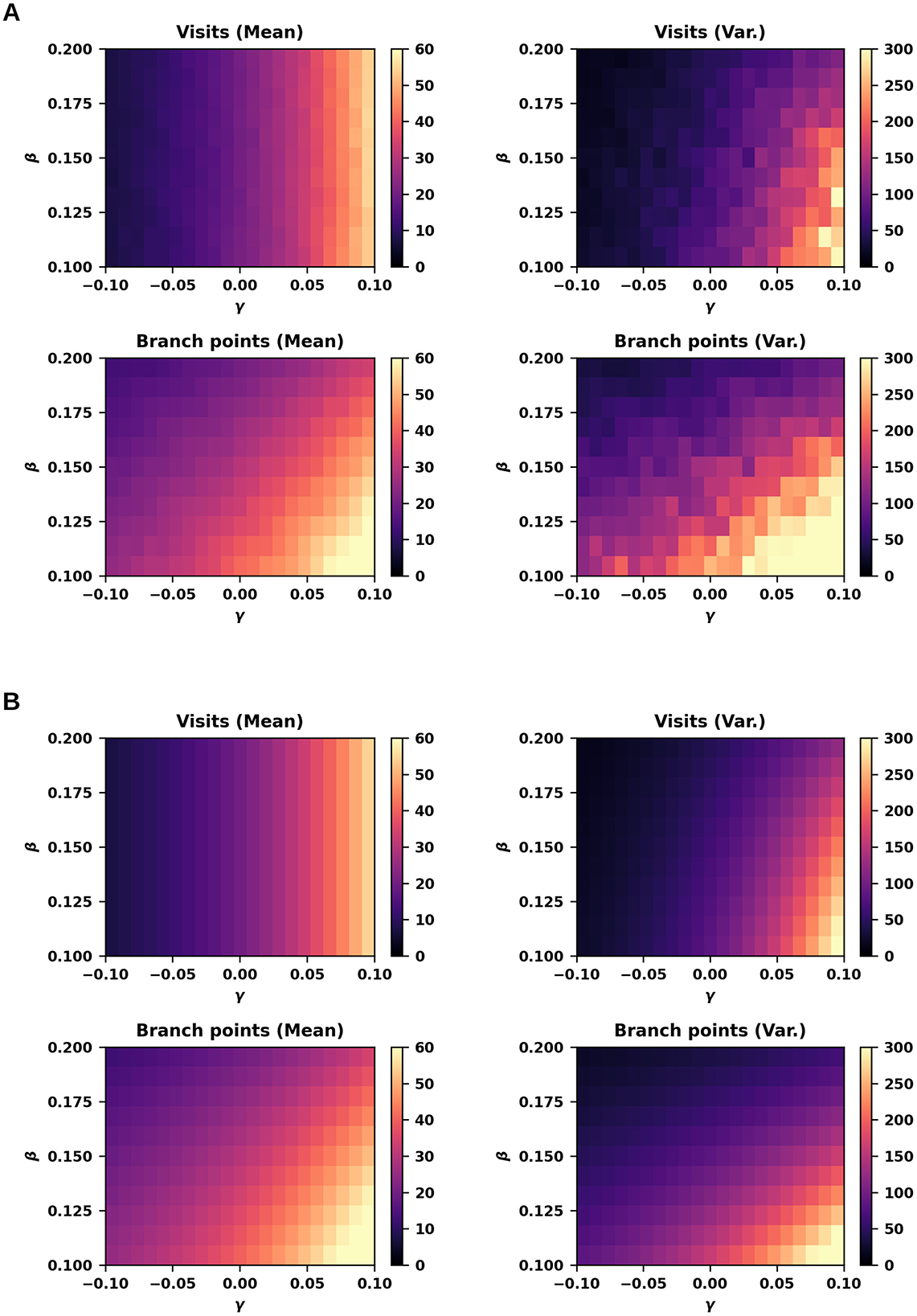
Figure 2. Number of visits and branch points under varying branching and annihilation rates. (A) Number of visits (top) and branch points (bottom) observed at the final iteration (t = 100, Δx = 0.1), starting from an initial number of branch points of 20 ± 2 (± SD), simulated using biased random walks (r = 1) across varying branching rates (β = 0.1 to 0.2) and net extension rates (i.e., difference between branching and annihilation rates; γ = β−α; γ = −0.1 to 0.1). For each parameter combination, the estimate is based on independent trials (n = 200). (B) Same as in panel (A), calculated by using equations.

4.1 Validation against experimental data

We tested our method using Sholl plots and branch point count of SL and PYR neurons from the piriform cortex of rats, obtained experimentally (SL: n = 3; PYR: n = 12) [6]. The choice of these cells is appropriate because their morphologies exhibit distinct and well-characterized branching patterns. These characteristics are captured by morphological metrics such as Sholl plots and branch point counts, which provide informative benchmarks for evaluating the performance of the model presented in this work. The comparison between simulation and experimental measures are shown in Figures 3A, B. Because these morphologies exhibited a very low percentage of segments oriented backwards (<0.1%), we excluded backward movements in random walk simulations, setting r = 1. Comparison of the means and variances of Sholl plots between simulations and experiments confirmed statistical indistinguishability for both cell types.

Figure 3

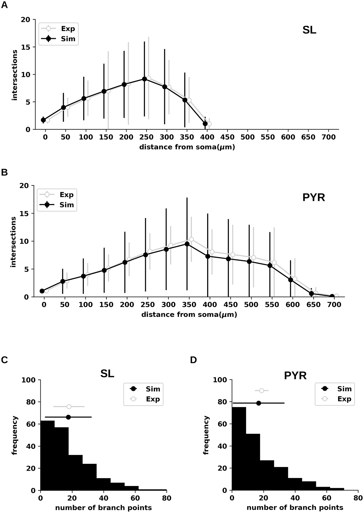
Figure 3. Sholl profiles and branch point counts for semilunar and pyramidal neurons from the piriform cortex generated by branching-and-annihilating random walks. (A) Sholl plots of semilunar (SL) neurons obtained from simulations (Sim; black) and experimental data (Exp; gray). Both means and variances were statistically indistinguishable between simulations and experiments across all spatial intervals. The simulation estimate is based on multiple independent trials (n = 200), with a step size Δx = 0.1. (B) Same as in (A), for pyramidal (PYR) neurons. Both means and variances were statistically indistinguishable between simulations and experiments across all spatial intervals. (C) Distribution of branch point counts for SL neurons obtained from simulations (black histogram and error bars) compared to experimental data (gray error bars). Both means and variances were statistically indistinguishable between simulations and experiments. (D) Same as in (C), for PYR neurons. Only the variances of simulations and experiments were statistically distinguishable (p < 0.001).

We then compared mean and variance for the branch point count between simulations (SL: 17.6 ± 14.8 (± SD); PYR: 16.9 ± 16.4) and experimental data (SL: 18.0 ± 9.9, n = 3; PYR: 18.8 ± 4.3 (± SD), n = 12) (Figures 3C, D). Significantly higher variance in simulated vs. experimental values was detected only in PYR neurons (p < 0.0001). (Figure 3D, compare gray and black). To exclude the possibility that this difference arose from the stochastic nature of the simulations, we compared mean and variance values of both Sholl plots and branch point counts from the simulations against their theoretical values (i.e., calculated through Equations 11, 13–15), confirming the absence of significant differences. To assess robustness, we varied the weight of the slack variable w over a broad range (0–100) and observed no effect on the fitting outcome. Instead, significantly lower variances were observed in experimental vs. theoretical values for Sholl plots (10/15 bins; p < 0.0001) and branch point count (p < 0.0001). These observations indicate that the differences between simulated and experimental values observed for PYR neurons were due to poor fitting. Furthermore, similar results were obtained when testing the model across additional morphologies (Supplementary Figures S1, S2), with a consistent tendency to exhibit higher variances than those observed experimentally for certain morphological types. Overall, these results support the ability of our model to replicate experimentally derived Sholl profiles, along with branch point counts, while highlighting the need for further refinement to better capture sources of morphological variability (see Discussion).

5 Discussion

In this study, we have introduced a mathematical framework that establishes a direct mapping between experimentally measurable quantities - Sholl plots and branch point counts - and the parameters governing branching-and-annihilating random walks. By turning these statistical descriptors into explicit constraints, the problem is reformulated from one of stochastic parameter fitting into a well-defined inverse problem, providing a rigorous foundation for extending morphology synthesis to diverse datasets and brain regions.

Our previous work demonstrated that branching-and-annihilating random walks can effectively synthesize realistic neuron morphologies [1, 3]. In this method, branching and annihilation rates were parameterized by branch depth; Sholl plots and branch point counts were treated as emergent properties. In particular, the specific random paths influenced the resulting Sholl plots, necessitating the empirical estimation of parameters through repeated trials. Here, we provide the mathematical bases to treat these descriptors as constraints rather than emergent outcomes. This eliminates path dependence and ensures their replication, thereby making the generation process more robust and reliable.

5.1 Comparison with existing methods

Numerous methods have been developed for neuron morphology synthesis, while only a minority are truly data-driven. Among these, the Topological Neuron Synthesis method constrains branch point positions using the Topological Morphology Descriptor (TMD) [17], while the TREES Toolbox generates morphologies from carrier points under the assumption that dendrites extend toward putative synaptic targets [16]. In the latter, the number of branch points depends directly on the number of carrier points [24], and morphologies are shaped by a single balancing factor that trades off material cost against conduction time [16, 24].

In contrast, our framework introduces two independent constraints: Sholl plots (compulsory) and branch point counts (optional) (see Equation 16). This separation allows branch point counts to be adjusted without altering Sholl profiles, providing finer control over morphology generation. Moreover, because it leverages commonly reported morphological metrics, our method enables data-driven synthesis without requiring detailed reconstructions. Together, these features make our framework more flexible and broadly applicable than existing approaches.

5.2 Mathematical contributions

From a mathematical standpoint, we introduce a problem-independent set of equations that link experimental summary statistics to the parameters of branching-and-annihilating random walks. By recasting the random walk dynamics as a Galton–Watson process, we derive closed-form expressions for the mean and variance of the branch-point count, supported by rigorous proofs. To the best of our knowledge, this is the first framework to establish such a direct and mathematically rigorous connection between experimental measurements and generative models of neuronal morphology. Importantly, the equations for the branch-point count in a Galton–Watson process are themselves new contributions.

5.3 Validation against experimental data

We validated the equations against experimental data (Figure 3; Supplementary Figures S1, S2). The resulting fits produced random walks with higher variance in both Sholl plots and branch point counts than those observed experimentally, although the differences were not significant. This outcome is consistent with expectations, as real morphologies emerge from complex developmental processes, whereas our approach is purely phenomenological and does not capture all aspects of dendritic extension. We speculate that the smaller variance observed experimentally reflects the action of additional biological constraints that reduce variability. Future work may address this limitation by incorporating such constraints into the model. However, this will require the knowledge of exact mechanisms and biochemical reactions that regulate dendritic growth, which still remains unknown.

6 Conclusion

In the immediate future, we plan to develop a toolbox that allows morphological synthesis based on the equations presented here. This toolbox will provide a practical platform for generating synthetic neuron morphologies that adhere to experimental constraints. It will also incorporate additional determinants of dendritic architecture that arise in three-dimensional space, including self-avoidance, spatial competition, branching-angle distributions, and dendritic tortuosity. Furthermore, the toolbox will account for geometric features that strongly influence electrotonic properties, such as total dendritic length and diameter tapering. Ensuring that synthetic morphologies replicate these characteristics will be critical for constructing realistic models of neuronal integration and network dynamics. As an initial application, we will focus on building biophysically detailed reconstructions of brain regions, beginning with the anterior piriform cortex, with the ultimate goal of enabling anatomically grounded large-scale simulations.

Data availability statement

The datasets presented in this study can be found in online repositories. The names of the repository/repositories and accession number(s) can be found below: https://github.com/FrancescoCavarretta/NeuronSynthesis.

Author contributions

FC: Conceptualization, Data curation, Formal analysis, Funding acquisition, Investigation, Methodology, Project administration, Resources, Software, Supervision, Validation, Visualization, Writing – original draft, Writing – review & editing.

Funding

The author(s) declare that no financial support was received for the research and/or publication of this article.

Conflict of interest

The author declares that the research was conducted in the absence of any commercial or financial relationships that could be construed as a potential conflict of interest.

Generative AI statement

The author(s) declare that no Gen AI was used in the creation of this manuscript.

Any alternative text (alt text) provided alongside figures in this article has been generated by Frontiers with the support of artificial intelligence and reasonable efforts have been made to ensure accuracy, including review by the authors wherever possible. If you identify any issues, please contact us.

Publisher's note

All claims expressed in this article are solely those of the authors and do not necessarily represent those of their affiliated organizations, or those of the publisher, the editors and the reviewers. Any product that may be evaluated in this article, or claim that may be made by its manufacturer, is not guaranteed or endorsed by the publisher.

Supplementary material

The Supplementary Material for this article can be found online at: https://www.frontiersin.org/articles/10.3389/fams.2025.1632271/full#supplementary-material

References

1. Migliore M, Cavarretta F, Hines ML, Shepherd GM. Distributed organization of a brain microcircuit analyzed by three-dimensional modeling: the olfactory bulb. Front Comput Neurosci. (2014) 8:50. doi: 10.3389/fncom.2014.00050

PubMed Abstract | Crossref Full Text | Google Scholar

2. Markram H, Muller E, Ramaswamy S, Reimann MW, Abdellah M, Sanchez CA, et al. Reconstruction and simulation of neocortical microcircuitry. Cell. (2015) 163:456–92. doi: 10.1016/j.cell.2015.09.029

PubMed Abstract | Crossref Full Text | Google Scholar

3. Cavarretta F, Burton SD, Igarashi KM, Shepherd GM, Hines ML, Migliore M. Parallel odor processing by mitral and middle tufted cells in the olfactory bulb. Sci Rep. (2018) 8:7625. doi: 10.1038/s41598-018-25740-x

PubMed Abstract | Crossref Full Text | Google Scholar

4. Dura-Bernal S, Neymotin SA, Suter BA, Dacre J, Moreira JV, Urdapilleta E, et al. Multiscale model of primary motor cortex circuits predicts in vivo cell-type-specific, behavioral state-dependent dynamics. Cell Rep. (2023) 42:112574. doi: 10.1016/j.celrep.2023.112574

PubMed Abstract | Crossref Full Text | Google Scholar

5. Grudt TJ, Perl ER. Correlations between neuronal morphology and electrophysiological features in the rodent superficial dorsal horn. J Physiol. (2002) 540:189–207. doi: 10.1113/jphysiol.2001.012890

PubMed Abstract | Crossref Full Text | Google Scholar

6. Bathellier B, Margrie TW, Larkum ME. Properties of piriform cortex pyramidal cell dendrites: implications for olfactory circuit design. J Neurosci. (2009) 29:12641–52. doi: 10.1523/JNEUROSCI.1124-09.2009

PubMed Abstract | Crossref Full Text | Google Scholar

7. Papoutsi A, Kastellakis G, Psarrou M, Anastasakis S, Poirazi P. Coding and decoding with dendrites. J Physiol-Paris. (2014) 108:18–27. doi: 10.1016/j.jphysparis.2013.05.003

PubMed Abstract | Crossref Full Text | Google Scholar

8. Kastellakis G, Silva AJ, Poirazi P. Linking memories across time via neuronal and dendritic overlaps in model neurons with active dendrites. Cell Rep. (2016) 17:1491–504. doi: 10.1016/j.celrep.2016.10.015

PubMed Abstract | Crossref Full Text | Google Scholar

9. Poirazi P, Papoutsi A. Illuminating dendritic function with computational models. Nat. Rev. Neurosci. (2020) 21:303–21. doi: 10.1038/s41583-020-0301-7

PubMed Abstract | Crossref Full Text | Google Scholar

10. Suzuki N, Bekkers JM. Two layers of synaptic processing by principal neurons in piriform cortex. J Neurosci. (2011) 31:2156–66. doi: 10.1523/JNEUROSCI.5430-10.2011

PubMed Abstract | Crossref Full Text | Google Scholar

11. Papoutsi A, Kastellakis G, Poirazi P. Basal tree complexity shapes functional pathways in the prefrontal cortex. J Neurophysiol. (2017) 118:1970–1983. doi: 10.1152/jn.00099.2017

PubMed Abstract | Crossref Full Text | Google Scholar

12. Udvary D, Harth P, Macke JH, Hege HC, de Kock CP, Sakmann B, et al. The impact of neuron morphology on cortical network architecture. Cell Rep. (2022) 39:110677. doi: 10.1016/j.celrep.2022.110677

PubMed Abstract | Crossref Full Text | Google Scholar

13. Kirchner JH, Euler L, Fritz I, Castro AF, Gjorgjieva J. Dendritic growth and synaptic organization from activity-independent cues and local activity-dependent plasticity. Elife. (2025) 12:RP87527. doi: 10.7554/eLife.87527.3

Crossref Full Text | Google Scholar

14. Moubarak E, Inglebert Y, Tell F, Goaillard JM. Morphological determinants of cell-to-cell variations in action potential dynamics in substantia nigra dopaminergic neurons. J Neurosci. (2022) 42:7530–46. doi: 10.1523/JNEUROSCI.2331-21.2022

PubMed Abstract | Crossref Full Text | Google Scholar

15. Zang Y, Marder E. Neuronal morphology enhances robustness to perturbations of channel densities. Proc Nat Acad Sci. (2023) 120:e2219049120. doi: 10.1073/pnas.2219049120

PubMed Abstract | Crossref Full Text | Google Scholar

16. Cuntz H, Forstner F, Borst A, Häusser M. One rule to grow them all: a general theory of neuronal branching and its practical application. PLoS Comput Biol. (2010) 6:e1000877. doi: 10.1371/journal.pcbi.1000877

PubMed Abstract | Crossref Full Text | Google Scholar

17. Kanari L, Dictus H, Chalimourda A, Arnaudon A, Van Geit W, Coste B, et al. Computational synthesis of cortical dendritic morphologies. Cell Rep. (2022) 39:110586. doi: 10.1016/j.celrep.2022.110586

PubMed Abstract | Crossref Full Text | Google Scholar

18. Berchet A, Petkantchin R, Markram H, Kanari L. Computational generation of long-range axonal morphologies. Neuroinformatics. (2025) 23:3. doi: 10.1007/s12021-024-09696-0

PubMed Abstract | Crossref Full Text | Google Scholar

19. Ascoli GA, Donohue DE, Halavi M. NeuroMorpho Org: a central resource for neuronal morphologies. J Neurosci. (2007) 27:9247–51. doi: 10.1523/JNEUROSCI.2055-07.2007

PubMed Abstract | Crossref Full Text | Google Scholar

20. Igarashi KM, Ieki N, An M, Yamaguchi Y, Nagayama S, Kobayakawa K, et al. Parallel mitral and tufted cell pathways route distinct odor information to different targets in the olfactory cortex. J Neurosci. (2012) 32:7970–85. doi: 10.1523/JNEUROSCI.0154-12.2012

PubMed Abstract | Crossref Full Text | Google Scholar

21. Davison AC, Hinkley DV. Bootstrap Methods and Their Application. 1 Cambridge: Cambridge university press. (1997). doi: 10.1017/CBO9780511802843

Crossref Full Text | Google Scholar

22. Allen LJS. Continuous-time birth and death chains. In: An Introduction to Stochastic Processes with Applications to Biology. Boca Raton: CRC Press (2010). p. 241–296.

Google Scholar

23. Wen Q, Stepanyants A, Elston GN, Grosberg AY, Chklovskii DB. Maximization of the connectivity repertoire as a statistical principle governing the shapes of dendritic arbors. Proc Nat Acad Sci. (2009) 106:12536–41. doi: 10.1073/pnas.0901530106

PubMed Abstract | Crossref Full Text | Google Scholar

24. Cuntz H, Mathy A, Häusser M. A scaling law derived from optimal dendritic wiring. Proc Nat Acad Sci. (2012) 109:11014–8. doi: 10.1073/pnas.1200430109

PubMed Abstract | Crossref Full Text | Google Scholar