 Aram Kamal Faraj1,2*
 Aso M. Aladdin
 Azad A. Ameen
- 1Department of Computer Science, College of Science, Charmo University, Sulaimani, Chamchamal, KR, Iraq
- 2Department of IT, Technical College of Informatics, Sulaimani Polytechnic University, Sulaimani, KR, Iraq
- 3Department of Software Engineering, College of Engineering and Computational Science, Charmo University, Chamchamal, Iraq
The fitness-dependent optimizer (FDO) has recently gained attention as an effective metaheuristic for solving different optimization problems. However, it faces limitations in exploitation and convergence speed. To overcome these challenges, this study introduces two enhanced variants: enhancing exploitation through stochastic boundary for FDO (EESB-FDO) and enhancing exploitation through boundary carving for FDO (EEBC-FDO). In addition, the ELFS strategy is proposed to constrain Levy flight steps, ensuring more stable exploration. Experimental results show that these modifications significantly improve the performance of FDO compared to the original version. To evaluate the performance of the EESB-FDO and EEBC-FDO, three primary categories of benchmark test functions were utilized: classical, CEC 2019, and CEC 2022. The assessment was further supported by the application of statistical analysis methods to ensure a comprehensive and rigorous performance evaluation. The performance of the proposed EESB-FDO and EEBC-FDO algorithms was evaluated through comparative analysis with several existing FDO modifications, as well as with other well-established metaheuristic algorithms, including the Arithmetic Optimization Algorithm (AOA), the Learner Performance-Based Behavior Algorithm (LPB), the Whale Optimization Algorithm (WOA), and the Fox-inspired Optimization Algorithm (FOX). The statistical analysis indicated that both EESB-FDO and EEBC-FDO exhibit better performance compared to the aforementioned algorithms. Furthermore, a final evaluation involved applying EESB-FDO and EEBC-FDO to four real-world optimization problems: the gear train design problem, the three-bar truss problem, the pathological igg fraction in the nervous system, and the integrated cyber-physical attack on a manufacturing system. The results demonstrate that both proposed variants significantly outperform both the FDO and the modified fitness-dependent optimizer (MFDO) in solving these complex problems.
1 Introduction
In real-world scenarios, optimization plays a vital role in solving complex problems across diverse fields such as engineering design, healthcare, transportation, energy systems, and machine learning. Many of these problems are difficult to solve using traditional mathematical approaches, particularly when the search space is large, non-linear, or contains multiple local optima. Metaheuristic algorithms have therefore emerged as powerful tools, providing efficient and flexible methods to approximate optimal solutions in practical applications [1–4]. Over the past two decades, metaheuristic algorithms have gained prominence due to their ability to handle complex, high-dimensional problems. They generally operate by applying strategic rules to candidate solutions, starting from randomly generated points and iteratively improving them through evaluation and comparison [5]. One of the earliest milestones in this field was John Holland's genetic algorithm (GA), developed in the 1960s and later published in the 1970s and 1980s [6–8]. This was followed by simulated annealing (SA) [9], inspired by the annealing process in metallurgy, and particle swarm optimization (PSO) [5, 10], inspired by the collective behavior of birds. These pioneering algorithms demonstrated strong potential for addressing real-world optimization challenges by finding high-quality solutions, reducing computational time, and overcoming local optima.
Since then, numerous algorithms have been introduced, such as the pathfinder algorithm (PFA) [11], the mayfly algorithm (MA) [12], the bear smell search algorithm (BSSA) [13], the gradient-based optimizer (GBO) [14], the group teaching optimization algorithm (GTOA) [15], the heap-based optimizer (HBO) [16], the Henry gas solubility optimization (HGSO) [17], the marine predators algorithm (MPA) [18], the political optimizer (PO) [19] the atom search optimization (ASO) [20], the Aquila optimizer (AO) [21], the herd optimization algorithm (HOA) [22], the Ebola optimization search algorithm (EOSA) [23] and the single candidate optimizer (SCO) [24]. The large number of algorithms can be attributed to the fact that no specific algorithm can be applied to all optimization problems, as pointed out in the no free lunch (NFL) theorem [25]. This theorem has logically demonstrated that no single algorithm is universally optimal for solving all types of optimization problems. The outcomes of these algorithms show that some achieve better results than others for certain specific problems [26].
A recurring theme in the design of these algorithms is the balance between exploration and exploitation [27–29]. Achieving a balance between these concepts is critical for improving algorithmic performance, as it enhances the ability of algorithms to converge efficiently while avoiding local optima. One of the primary limitations of the fitness-dependent optimizer (FDO) algorithm, as identified in previous studies, is its underdeveloped exploration capability, which has prompted significant research efforts aimed at addressing this issue. This paper emphasizes improving exploitation while maintaining a strong focus on exploration. To confine the algorithm within a specified search space defined by lower and upper bounds after updating the bees' positions, the FDO algorithm utilizes a specialized function called the “getBoundary” function [30, 31]. This function effectively transforms outlier values of bee positions into feasible values within the defined boundaries. By introducing modifications to the equations within the “getBoundary” function, this study aims to enhance the FDO algorithm's performance, contributing to more efficient optimization outcomes.
The main contributions of this study can be summarized as follows:
1. Proposed two novel boundary handling strategies for the Fitness fitness-dependent optimizer (FDO):
• EESB-FDO: Enhancing exploitation through stochastic repositioning, which introduces random values within bounds when scout bees exceed search space limits.
• EEBC-FDO: Enhancing exploitation through boundary carving, which redirects bees toward feasible regions using boundary carving equations.
2. Introduced the ELFS strategy, which modifies the Levy flight mechanism to restrict step sizes within a bounded range, preventing instability due to excessive jumps.
3. Conducted extensive benchmarking using classical, CEC 2019, and CEC 2022 test functions, demonstrating significant improvements in exploitation capability and convergence behavior.
4. Applied the proposed variants to four real-world engineering problems, proving their practical its effectiveness in solving complex, constrained optimization scenarios.
5. Performed comparative statistical analysis with state-of-the-art algorithms, confirming the competitiveness and reliability of EESB-FDO and EEBC-FDO under various optimization challenges.
The remaining sections of this paper are organized as follows: Section 2 presents a review of related work on the FDO. Section 3 provides a detailed description of the FDO algorithm. In Section 4, the proposed methodology is explained, followed by the introduction of the FDO modifications in Section 5. Section 6 presents the experimental results and comparisons with other algorithms using a set of benchmark test functions. Finally, Section 7 summarizes the main findings and offers directions for future research.
2 Related work
Advancing the FDO recently and effectiveness in solving real-world problems demonstrate that it is one of the most powerful metaheuristic algorithms in recent years [32–35]. Additionally, it uses random walk techniques, such as Levy flight [3], which have been employed in prior studies to improve the performance of the optimization of other algorithms. Selecting an appropriate equation or method is crucial for efficiently reaching the global optimum while avoiding local optima. Following the development of any new algorithm, the modification and enhancement of existing algorithms using various methods and techniques are critical steps commonly undertaken by researchers to improve performance and adaptability. For example, the GA [36] has been extended to the adaptive genetic algorithm (AGA) [37], and PSO [10] has evolved into the comprehensive learning PSO (CLPSO) [38]. Similarly, the ant colony optimization (ACO) [39] method was improved to the max–min ant system (MMAS) [40], while the FA [2] was adapted into the adaptive firefly algorithm (AFA) [41], and AOA [42] was refined into the enhanced AOA (EAOA) [43].
The enhancement and generation of algorithms are increasing rapidly; this rapid expansion has necessitated the need to manage and categorize them. There are various ways to classify these algorithms, and one common approach is based on their source of inspiration, which can be either natural or non-natural. Nature-inspired metaheuristic algorithms can be broadly categorized into four main classes: physics-based algorithms, evolutionary algorithms, human-based algorithms, and swarm-based algorithms [44]. The FDO is a metaheuristic algorithm that belongs to the swarm-based algorithms group, inspired by the bee swarming reproductive process. More specifically, it can be seen as an extension of PSO [31]. Various methods and techniques have been employed to enhance and improve the performance of the FDO algorithm, and these improvements must be acknowledged. Adding two parameters (alignment and cohesion) to update the position of search agents in addition to the existing pace factor [32]. Ten chaotic maps have been used for the initialization population, which is another improvement implemented in FDO [45]. After that, updating pace (velocity) by utilizing the sine–cosine scheme, modified pace-updating equations in the search phase, random weight factor, global fitness weight strategy, conversion parameter strategy, and the best solution-updating strategy[33]. Then, modifying the fitness-dependent optimizer by changing waited factor range from [0,1] to [0,0.2] is another mechanism [34].
With these developments and improvements, the FDO algorithm has been effectively applied to solve and address a variety of problems, demonstrating significant success in finding optimal solutions. For instance, the adaptive fitness-dependent optimizer has been applied to the one-dimensional bin packing problem, an NP-hard problem, producing more promising results compared to other approaches [46]. Subsequently, the automatic generation control (AGC) of a multi-source interconnected power system (IPS) was more effectively managed using FDO, reducing frequency overshoot/undershoot and settling time [47]. Then Improved-FDO was applied to control the same problem and provide better results than FDO [48]. Building on the advantages of FDO in controlling Automatic Generation Control (AGC), a new controller called the “modified PID controller” is introduced, which achieves more effective control than before, again utilizing FDO [49]. The performance of this algorithm was further leveraged to enhance another area, specifically in multilayer perceptron (MLP) neural networks, resulting in an increase in the average accuracy of the model [50]. FDO has demonstrated superior efficiency in solving non-linear optimal control problems (NOCPs) compared to the GA algorithm, effectively minimizing absolute error and providing better solutions [51].
A new technique called generalized regression neural network combined with fitness-dependent optimization (GRNNFDO) has been used to control the behavior of the thermoelectric generator (TEG) system, and this technique produces more power compared to other algorithms [52]. The economic load dispatch (ELD) problem is another area where the improved FDO has been used to effectively reduce emission allocation and fuel costs [53]. Another effective method for classifying COVID-19 cases as positive or negative, where FDO combined with neural networks was tested on three different datasets, enhanced accuracy rates and minimized error rates [54]. A hybrid approach combining genetic algorithm and FDO (GA-MFDO) has been used to solve the NP-hard problem of workflow scheduling, achieving a significant p-value compared to other methods [55]. Similarly, the edge server allocation problem, an NP-hard challenge, was effectively addressed using the effective fitness-dependent optimizer (EFDO). When tested on Shanghai Telecom's dataset, which includes factors such as access delay, energy consumption, and workload balance, EFDO outperformed competing algorithms [56]. Finally, FDO integrated with neural networks has also been employed for detecting steel plate faults, achieving higher classification accuracy than other methods [57].
Levy flight is a type of random walk where step lengths follow a Levy distribution, characterized by its heavy-tailed probability distribution. It is one of the most effective approaches for generating a diverse and well-distributed random initialization set, thereby enhancing the exploration capabilities of the algorithm when metaheuristic algorithms begin with a randomly initialized set of values, structured according to the algorithm's design and procedural steps [2]. Levy flight is a fundamental component of the cuckoo search (CS) algorithm, which mimics the foraging behavior of certain animals and insects [58]. In this work, Levy flight is utilized to simulate insect movement, significantly boosting the global search capability of the flower pollination algorithm (FPA) [59]. For algorithms like the dragonfly algorithm (DA), Levy flight guides stochastic behavior, allowing for better traversal of the search space [60]. Additionally, the combination of differential evolution (DE) and Levy flight (LF) techniques has been shown to improve the performance of the harmony search algorithm (HSA) [61]. The slap swarm algorithm (SSA) also benefits from Levy flight mutation, which enhances its randomness and exploration capabilities during the search process [62]. Similarly, Levy flight-based mutation has been introduced to improve the exploration ability and overall efficiency of the slime mould algorithm (SMA) [63]. Furthermore, the use of Levy flight in the bat algorithm (BA) has been shown to improve its ability to escape local optima and achieve faster convergence [64] Similarly, the incorporation of Levy flight in the gray wolf optimizer (GWO) enhances its global search ability, making it more effective for solving complex optimization problems [65].
3 FDO algorithm
The FDO is inspired by the swarming behavior of bees during colony reproduction. When bees seek to establish a new hive, they follow a systematic set of rules to identify a suitable location. These decision-making processes within the bee community can be categorized into two fundamental components: searching for an appropriate site and moving toward it. Further details regarding FDO are provided through its parameter settings, as summarized in Table 1. These parameters significantly influence the algorithm's performance, and deviations beyond their predefined values may adversely affect the quality of the results.
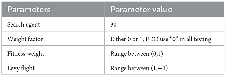
Table 1. FDO parameter settings.
In optimization algorithms, the search process is typically conducted within a predefined search space to identify optimal solutions. To ensure that the search remains within these boundaries, some algorithms implement a boundary handling mechanism. This mechanism involves iterating through potential solutions and adjusting any values that exceed the predefined limits by reassigning them to a random boundary value. This section provides a detailed exploration of these three key aspects: searching, movement, and boundary handling. Showed Pseudo code of FDO in Figure 1.
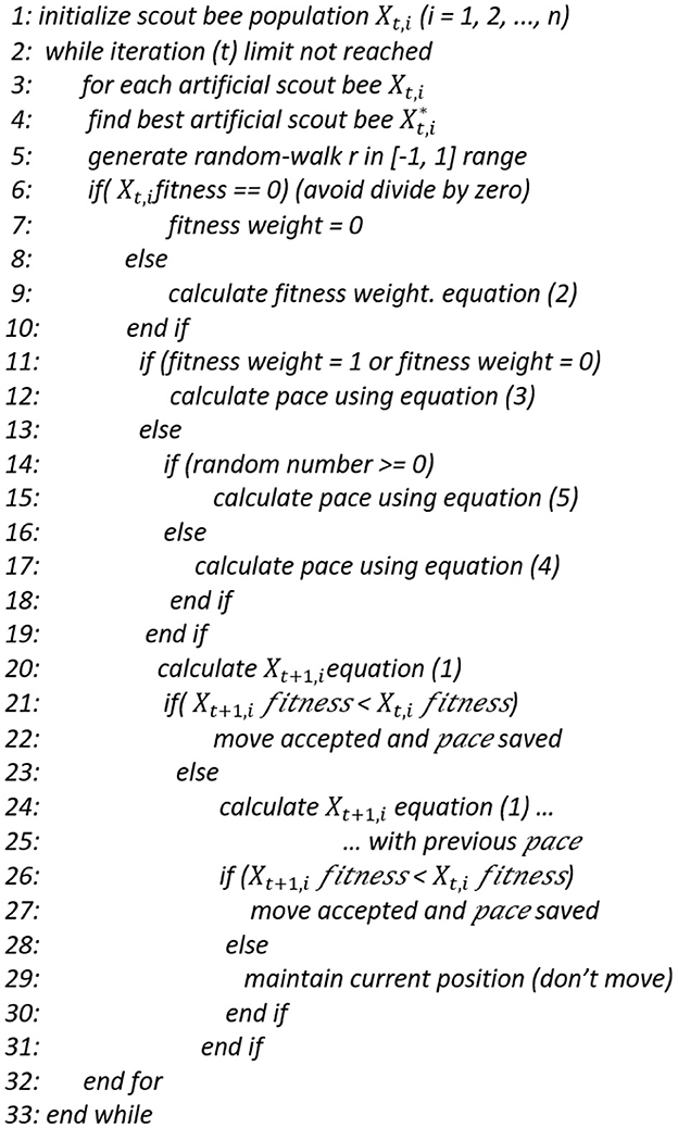
Figure 1. Pseudo code of FDO described in Abdullah and Ahmed [31].
3.1 Bee searching
Scout bees initiate the search for an optimal hive by exploring various potential locations. This process represents a fundamental stage in the algorithm, which begins with the random generation of the scout bee population within a predefined search space, denoted as Xi(where i = 1, 2, 3, …, n). Each scout bee's position corresponds to a newly discovered solution within the search space. To identify a more suitable hive, scout bees perform a stochastic search for alternative locations. If a newly identified position offers a more favorable solution, the previous locations are disregarded. Conversely, if the new position does not yield an improvement, the scout bees continue moving in their prior direction while disregarding the less optimal locations.
3.2 Bee movement
In the natural world, scout bees search for a hive randomly to identify a more suitable location for reproduction. Similarly, artificial scout bees adopt this principle by moving and updating their current position to a potentially improved one through the addition of a pace value. If the newly discovered solution proves to be superior to the previous one, the scouts proceed in the current direction; otherwise, they continue following their prior trajectory. The movement of artificial scout bees is determined using Equation 1.
where i represents the current search agent, t represents the current iteration, x represents an artificial scout bee (search agent), and pace is the movement rate and direction of the artificial scout bee. The fitness weight (fw) as expressed in Equation 2 is used to calculate and manage the pace when the direction of pace is completely dependent on a random mechanism.
where denotes the best global solution's fitness function value that has been revealed so far; denotes the current solution's value of the fitness function; and wf denotes a weight factor, randomly set between 0 and 1, which is used for controlling the fw.
Later, the algorithm considers some settings for fw, for instance, if fw = 1 or 0, and = 0, the algorithm sets the pace randomly according to Equation 3. On the other hand, if fw > 0 and fw < 1, then the algorithm generates a random number in the (−1, 1) range to make the scout search in every direction; when r < 0, pace is calculated according to Equation 4, and when r >= 1, pace is calculated according to Equation 5.
where r denotes a random number in the range of [−1, 1], Xi, t denotes the current solution, and denotes the global best solution achieved thus far. Among various applications for random numbers, the FDO selects Levy flight because it considers further stable movement via its fair distribution curve [10].
3.3 Bee boundary
In optimization algorithms, the search space refers to the set of all possible solutions within which the algorithm seeks to identify the optimal solution. The algorithm explores this space to determine the most suitable outcome. Each algorithm operates within a defined search space, constrained by specific boundaries and limitations to ensure both efficiency and feasibility. The performance of an algorithm is significantly influenced by the structure of the search space, and maintaining the algorithm's operations within the prescribed boundaries is crucial for its success. For instance, the FDO utilizes mechanisms, such as Equations 6 and 7 to adjust values that exceed the defined range, ensuring that all solutions remain within the limited search space. This approach enhances the algorithm's ability to converge toward optimal solutions effectively.
where Xi, t+1 represent the new bee value after the update in each iteration, the upper bound represents the upper boundary value of search space, the lower bound represent the lower boundary value of search space, and Levy shows Levy flight to generate a random value between (−1,1).
4 Methodology
This section of the research outlines the study aimed at enhancing the FDO algorithm. It encompasses addressing exploitation limitations, improving FDO through adaptive bee update strategies, experimental setup, performance evaluation, and effectiveness assessment. The primary objective of this study is to improve the algorithm's exploitation capability, which has been identified as one of its main weaknesses, illustrated in Figure 2.
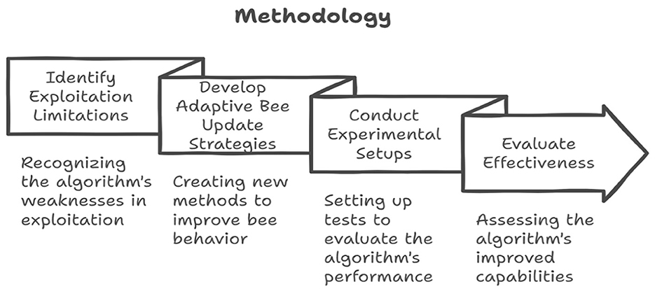
Figure 2. Explain methodology steps.
4.1 Addressing exploitation limitations
Optimization problems are prevalent across various specialized domains, where the primary objective is to identify the optimal solution among numerous possible alternatives. In the field of metaheuristic algorithms, enhancing both exploration and exploitation is essential for improving performance. Exploitation focuses on refining solutions within promising regions. The FDO has been observed to exhibit weaknesses in exploitation; theoretically, exploitation can be improved by concentrating the search around high-quality solutions. In the context of swarm-based algorithms, this involves reinforcing local search behavior while maintaining feasibility. The proposed modifications aim to increase solution density within promising regions, thereby enhancing the probability of convergence toward global optima. According to convergence theory in metaheuristics, increasing selective pressure around fitter solutions helps refine accuracy in late-stage optimization, limiting the algorithm's ability to converge efficiently toward optimal solutions. Therefore, this research aims to address and enhance the exploitation capability of the FDO algorithm to improve its overall effectiveness in solving complex optimization problems.
4.2 Improving FDO through adaptive bee update strategies
As discussed in the preceding sections, various methods and solutions have been employed to address this issue, contributing to a relative improvement in the exploitation capability of the FDO. This enhancement of the algorithm adds new progression to previous improvements by introducing some novel equations to update bees: that exceed the boundary of the search space. In this research, two new modifications are proposed for updating these exceeding bees, the first one, EESB-FDO, is designed to update bees, and the second, EEBC-FDO, also aims to update bees, both contributing to improving the exploitation capability of the FDO algorithm. From a theoretical standpoint, boundary handling mechanisms play a critical role in shaping the topology of the solution space. The proposed modifications replace rigid boundary clipping with stochastic repositioning or controlled correction strategies. These approaches improve the algorithm's capacity to recover from constraint violations while maintaining stable and coherent search dynamics. Such strategies are consistent with the principles of constrained optimization and contribute to preserving the continuity and efficiency of the search trajectory.
4.3 Experimental setup and performance evaluation
The algorithm was implemented in the MATLAB 2022 environment on a laptop equipped with a 10th-generation Intel Core i5 processor and 8 GB of RAM. After incorporating modifications, the algorithm was executed more than 30 times, each for 500 iterations. The performance was evaluated using a set of benchmark functions and statistical methods. The results demonstrate the improved efficiency of the algorithm with the proposed updates compared to its previous version.
4.4 Effectiveness assessment
The testing stage is crucial for evaluating the effectiveness and capability of the algorithm. This process consists of several key steps, including benchmark test functions, comparative analysis, statistical test methods, and real-world problem testing. Benchmark testing functions, such as classical, CEC2019, and CEC2022, are used to assess the performance and capability of the new improvements. Comparative analysis measures the enhanced algorithm's results against the original version and other existing algorithms. Additionally, statistical methods, including the Wilcoxon rank-sum test, standard deviation, and mean, are used to verify the significance, performance, consistency, and reliability of the algorithm. Real-world testing is conducted by applying the algorithm to practical problems. The testing phase ultimately confirms that the modifications have led to meaningful enhancements.
5 FDO modifications
In this section, this study focuses on three modifications: EESB-FDO, EEBC-FDO, and ELFS, which are proposed as extensions of the FDO. These modifications and FDO are substantive to parameter setting and change results by changing one of them [19]. The fundamental concept of FDO is inspired by the reproductive process and collective decision-making behavior exhibited by bees. Specifically, it mimics the way bees search for multiple available hives and collaboratively select the most optimal ones.
5.1 Enhancing FDO performance through scout bee boundary repositioning
The artificial scout bee operates on the same principle, searching for the optimal solution among multiple available options within the defined boundary search space. Maintaining the search within a restricted area is a crucial factor influencing the algorithm's performance and effectiveness. To enforce this condition, the FDO employs Equations 6 and 7. When the position of an artificial scout bee exceeds the predefined boundaries, the FDO updates its value according to these equations, ensuring that the search remains within the permitted limits. In this enhancement, two new modifications are proposed to update scout bees that exceed the upper or lower boundary, ensuring they remain within the predefined search space as described below.
5.1.1 Enhancing exploitation through stochastic boundary for FDO
The first modification employs Equation 8 to regulate values that surpass either the upper or lower boundary, meaning using just one Equation 8 instead of Equations 6, 7. By using this equation, EESB-FDO updates the bee value that exceeds the boundaries (upper and lower); the proposed approach utilizes a randomized value within a predefined fixed range. This involves generating random values within the defined search space limits, thereby introducing greater diversity and adaptability into the search process, as shown in Figure 3A. This approach leverages uniform random sampling within the valid bounds, which ensures all feasible regions are equally likely to be explored upon violation. This strategy preserves population diversity and prevents premature convergence caused by agents clustering near hard boundary limits. It also avoids stagnation by introducing controlled randomness, a key requirement for ergodicity in metaheuristic convergence.
Here, update Xi, t+1 represents the new bee value after update in each iteration, random (boundary) mean generate any random value in the predefined search space between the upper boundary and lower boundary, Levy flight to generate a random value between (−1,1).
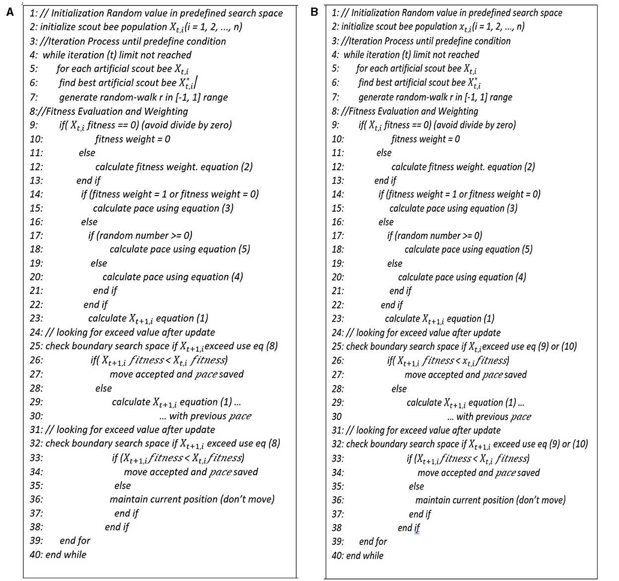
Figure 3. Pseudo code of FDO with (EESB) and (EEBC). (A) EESB-FDO. (B) EEBC-FDO.
5.1.2 Enhancing exploitation through boundary carving for FDO
The second modification utilizes Equation 9 to adjust values that exceed the upper boundary and Equation 10 to regulate values that fall below the lower boundary. By formulating two equations for updating scout bees, notable progress has been achieved in enhancing the algorithm's performance. These equations contribute to more effective handling of boundary violations and improve the overall exploitation capability of the algorithm, as explained in Figure 3B.
where updateXi, t+1 represents the new bee value after the update in each iteration, Xi, t+1 represents the old bee value that exceed boundaries, the upper bound represents the upper boundary value of the search space, the lower bound represents the lower boundary value of the search space, and Levy shows Levy flight to generate random values between (−1,1).
5.2 Eliminating levy flight shortcomings
Levy flight is a type of random walk where step lengths follow a Levy distribution, known for its heavy-tailed probability distribution, as shown in the pseudo code in Figure 4. This property makes Levy flight highly effective for exploring large and unknown search spaces [2].
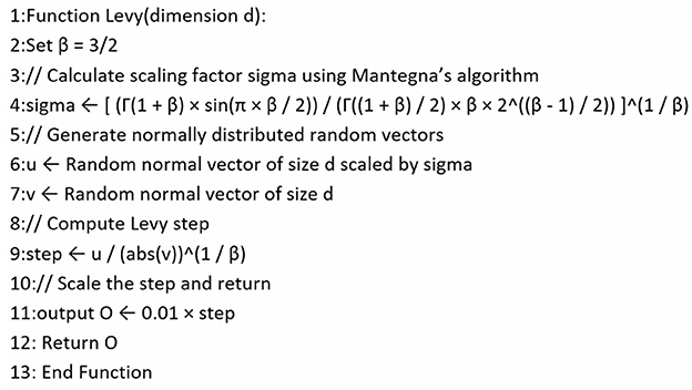
Figure 4. Pseudo code of Levy flight.
Levy flight represents a type of random walk and plays a crucial role in metaheuristic algorithms by generating random values within the range of (−1,1). However, these values should not exceed the defined limits. To assess the behavior of Levy flight, it was executed 30 times, each with 10,000 iterations. The results, as presented in Figure 5, indicate that in each execution, some randomly generated values exceeded the specified range of (−1,1). To address this issue, Equation 11 was incorporated into the Levy flight mechanism. This equation ensures that any generated value exceeding the upper limit of 1 is adjusted to 1, while any value falling below the lower limit of −1 is set to −1. In Figure 4, explaining Levy flight before enhancement, it was shown that O was represented by (0.01 × step) and then changed to Equation 11 after the update.
where O represents the output of the Levy flight function, Equation 11 ensures that the generated values remain within the defined range of (−1,1) without exceeding these limits.

Figure 5. Result of calling Levy flight 30 times.
6 Result and discussion
The key point of algorithm evaluation is the comparison with other established optimization methods. To ensure a comprehensive assessment, various evaluation metrics are employed, including benchmark functions, statistical methods, and real-world problem scenarios. In this study, the proposed EESB-FDO and EEBC-FDO were compared with seven metaheuristic algorithms: FDO [31], arithmetic optimization algorithm (AOA) [42], gravitational search algorithm (GSA) [66], GWO [65], learner performance-based behavior algorithm (LPB) [67], whale optimization algorithm (WOA) [68], and fox-inspired optimization algorithm (FOX) [69] using classical benchmark functions, CEC-2019, and CEC-2022. The performance evaluation is conducted based on statistical measures such as mean, standard deviation, and the Wilcoxon rank-sum test to ensure the performance and capability. To ensure fair and unbiased comparisons, all algorithms were evaluated under identical experimental conditions. Each algorithm was executed independently for 30 runs to account for the stochastic nature of metaheuristic methods. In every run, a population of 30 search agents was employed, and the optimization process was conducted for a maximum of 500 iterations. This consistent configuration across all algorithms ensures that observed performance differences are attributable to algorithmic effectiveness rather than variations in experimental settings. Following the execution, the average and standard deviation were calculated, and the results are presented in this section.
6.1 Classical benchmark test functions
The performance of EESB-FDO and EEBC-FDO was evaluated using three categories of test function groups, as outlined in Zervoudakis and Tsafarakis [12]. These test function groups possess distinct characteristics that assess different aspects of the algorithms' performance. Unimodal test functions (f1–f7) are employed to evaluate the algorithms' exploitation capability and convergence efficiency, as they contain only a single global minimum (or maximum) without any local optima, as shown in Table 2. In contrast, multimodal test functions (f8–f13) are utilized to assess the algorithms' exploration ability, ensuring they can escape local optima and effectively search for the global solution in complex landscapes with multiple optimal points, as presented in Table 3. Additionally, composite benchmark functions (f14–f23) are represent advanced test functions designed to simulate real-world optimization challenges, providing a more rigorous evaluation of the algorithms' robustness and adaptability in highly complex and irregular search spaces, as presented in Table 4.
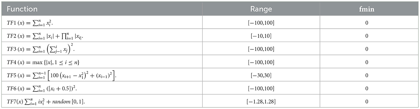
Table 2. Unimodal benchmark functions [80].
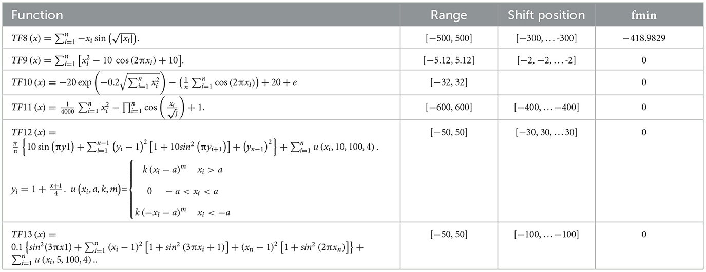
Table 3. Multi-modal benchmark functions [80].
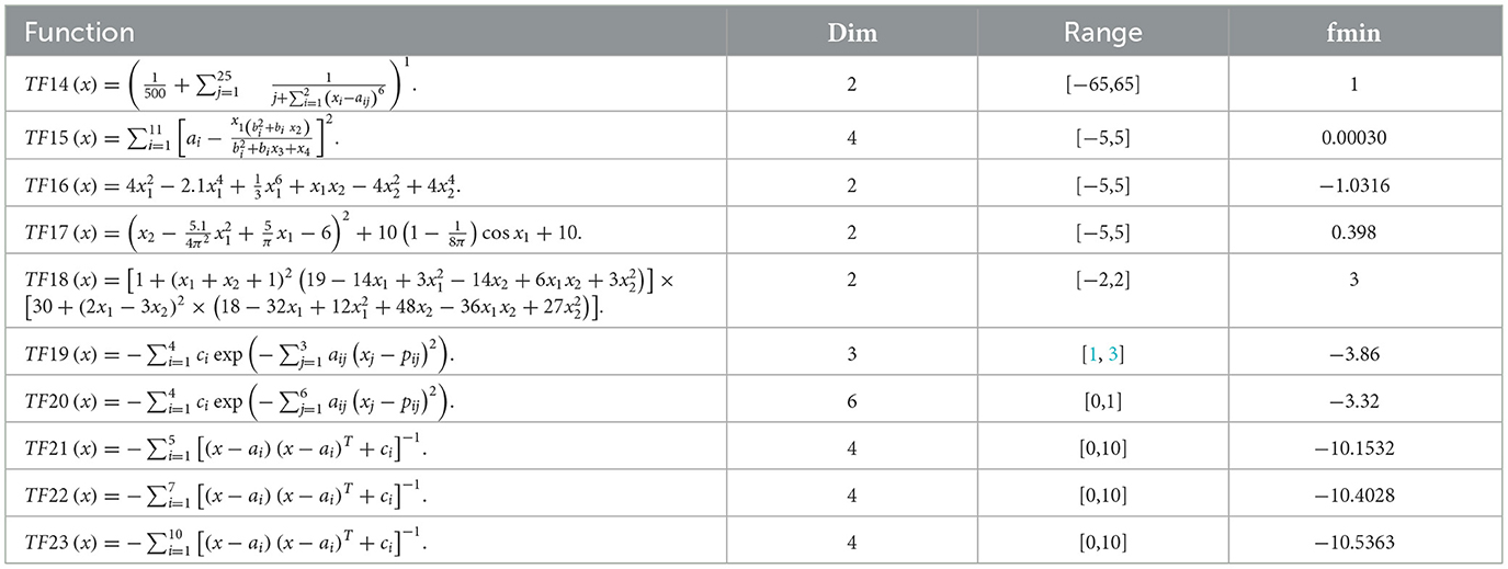
Table 4. Fixed-dimension multimodal benchmark functions [80].
All algorithms presented in Tables 5–10 were evaluated over 30 independent runs, each consisting of 500 iterations. The optimization process was initiated with 30 randomly generated search agents in 10, 20, and 30-dimensional search spaces for the first two test function groups (unimodal and multimodal functions). For the composite test function group, the dimensionality was set according to the structural requirements of each function. The performance of the algorithms was assessed by computing statistical measures, including the mean and standard deviation, to ensure a comprehensive evaluation of their optimization capabilities.
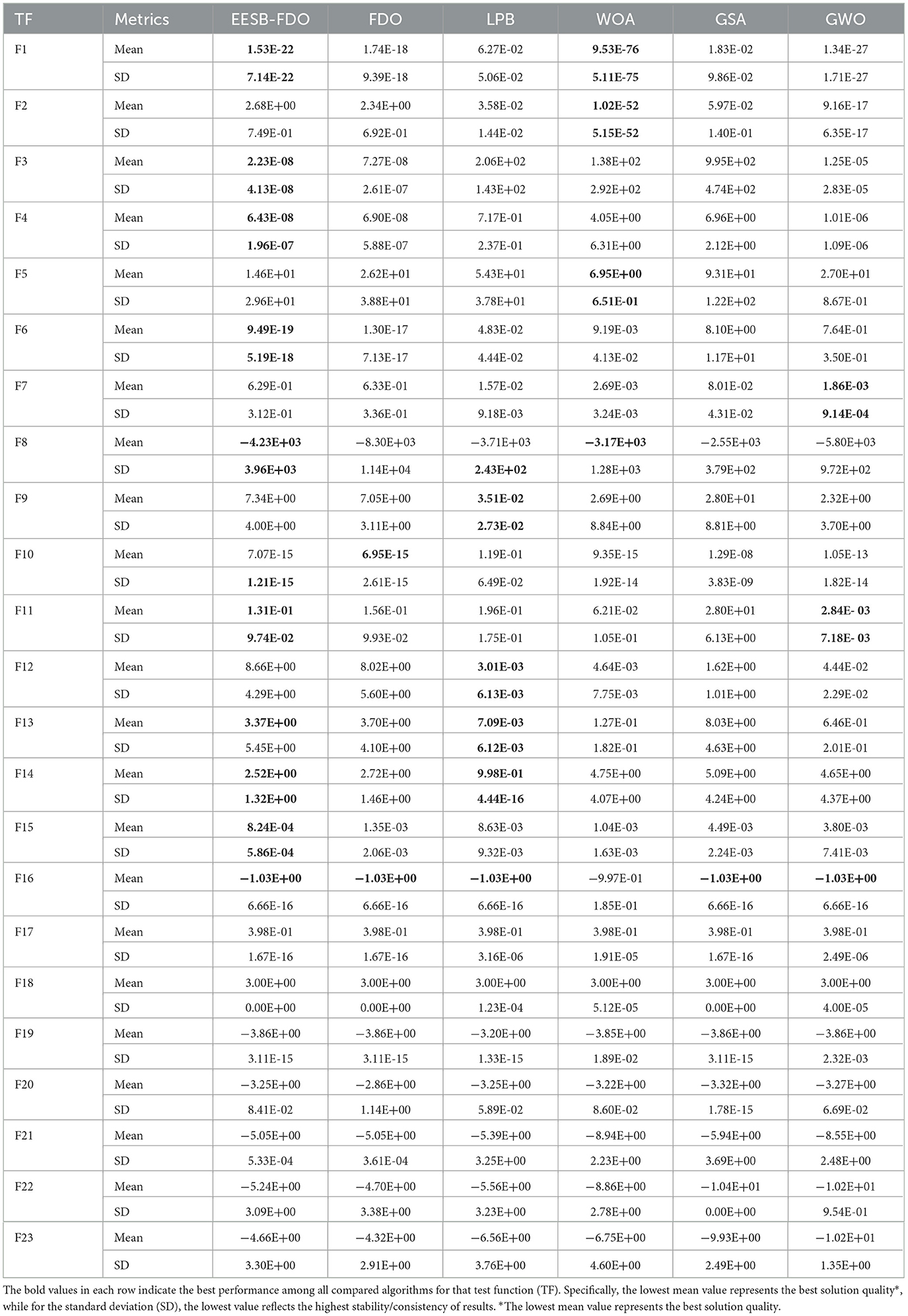
Table 5. Results of comparing EESB-FDO with FDO and other chosen algorithms using classical benchmark functions.
6.1.1 Classical benchmark test for enhancing exploitation through stochastic boundary for FDO
The results of EESB-FDO, FDO, LPB, WOA, GSA, and GWO, as shown in Table 5 for test functions TF1 to TF7, indicate that EESB-FDO generally outperforms FDO, with the exception of TF2. Specifically, EESB-FDO demonstrates superior performance over FDO, LPB, and GSA for TF1. Additionally, for TF3, TF4, and TF6, EESB-FDO outperforms all other algorithms. However, in TF2 and TF5, EESB-FDO shows comparatively poor performance, with other algorithms outperforming it. These results, by enhancing F1 to F7 static values, mean minimizing values and prove that the new modification in EESB-FDO significantly improves the algorithm's exploitation capability.
On the other hand, in TF8, TF11, TF14, and TF15, the results indicate that EESB-FDO outperformed FDO. However, when compared to other algorithms, the performance of these alternatives was slightly superior. Furthermore, in TF16, TF17, TF18, and TF19, both EESB-FDO and FDO achieved the optimal value and demonstrated comparable performance. In general, their results were more favorable than those of other algorithms.
In addition to the previous comparisons, Table 6 presents the results of EESB-FDO in comparison with M-IFDO, IFDO, SC-FDO, and CFDO. The findings indicate that EESB-FDO performed better than M-IFDO and IFDO in TF2 and TF4. In TF5, it outperformed all algorithms except SC-FDO, while in TF6, it demonstrated superior performance compared to the others. However, for TF1, TF3, and TF7, its results were the weakest among the algorithms. Furthermore, regarding multimodal functions, EESB-FDO achieved better performance than M-IFDO and IFDO in TF9, TF12, and TF13. However, in TF8, TF11, TF14, and TF15, its results fluctuated, showing slight weaknesses. Additionally, from TF16 to TF19, EESB-FDO successfully attained the optimal values, demonstrating its effectiveness in these test cases.
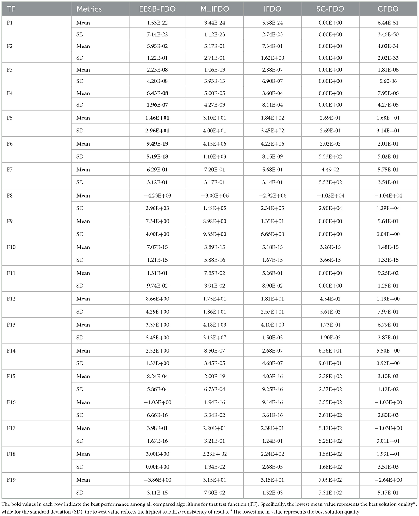
Table 6. Results of comparing EESB-FDO with modifications Of FDO using classical benchmark functions.
The final evaluation of EESB-FDO, in comparison with FDO, was conducted using both 20- and 30-dimensional settings across unimodal and multimodal benchmark test functions, as presented in Table 7. In the 20-dimensional case, EESB-FDO outperformed FDO on several functions, specifically F1, F2, F3, F5, F6, F10, and F11, indicating a clear advantage in terms of both convergence speed and exploitation capability within this dimensional context. In the 30-dimensional case, EESB-FDO demonstrated superior performance compared to FDO on several benchmark functions, namely F1, F2, F5, F6, F9, F12, and F13. These results highlight the algorithm's enhanced convergence speed and exploitation capability, underscoring its effectiveness in handling complex optimization tasks within this dimensional setting. The results clearly indicate that several benchmark functions showed significant improvement, approaching near-optimal solutions, following dimension modification and the discovery of new optimal points.
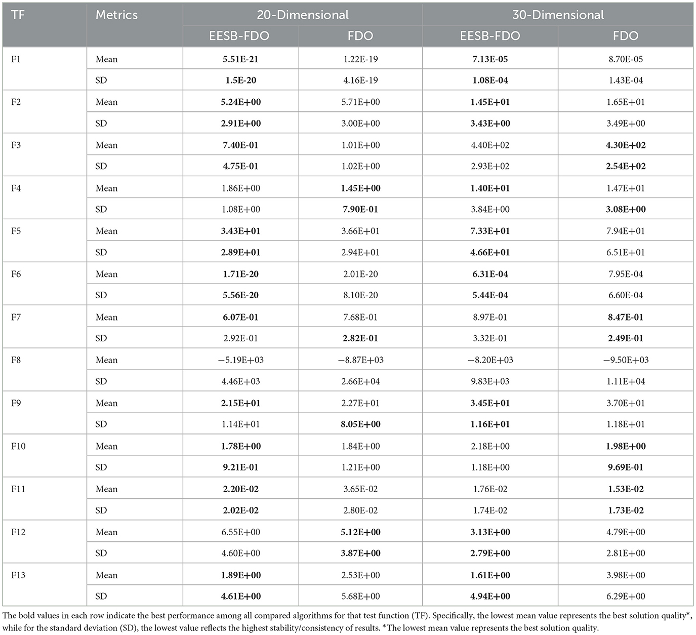
Table 7. Results of comparing EESB-FDO with FDO for (20 and 30) dimensions.
6.1.2 Classical benchmark test for enhancing exploitation through boundary carving for FDO
For the second modification, EEBC-FDO, the results presented in Table 8 clearly demonstrate its superiority over the FDO in TF1 to TF7, with the exception of TF3, where it outperformed other algorithms but performed worse than FDO. These outcomes indicate an improvement in the algorithm's exploration capability. Additionally, in TF1 and TF2, EEBC-FDO performed better than LPB and GSA but was outperformed by WOA and GWO. In TF4, TF5, and TF6, EEBC-FDO outperformed all other algorithms, demonstrating its competitive advantage. However, from TF9 to TF15, its performance showed slight weaknesses, except for TF10, where it performed favorably compared to other algorithms. Nonetheless, in TF16 to TF19, both FDO and EEBC-FDO achieved equal performance, obtaining the optimal value. On the other hand, Table 9 presents a comparison of EEBC-FDO with previous modifications of FDO, including M-IFDO, IFDO, SC-FDO, and CFDO. The results indicate that the performance of EEBC-FDO is closely aligned with that of EESB-FDO when compared to these modifications.
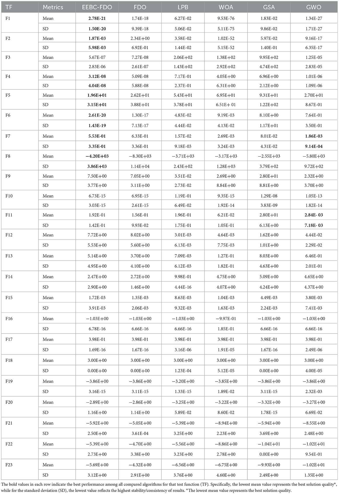
Table 8. Results of comparing EEBC-FDO with FDO and other chosen algorithms Using classical benchmark functions.
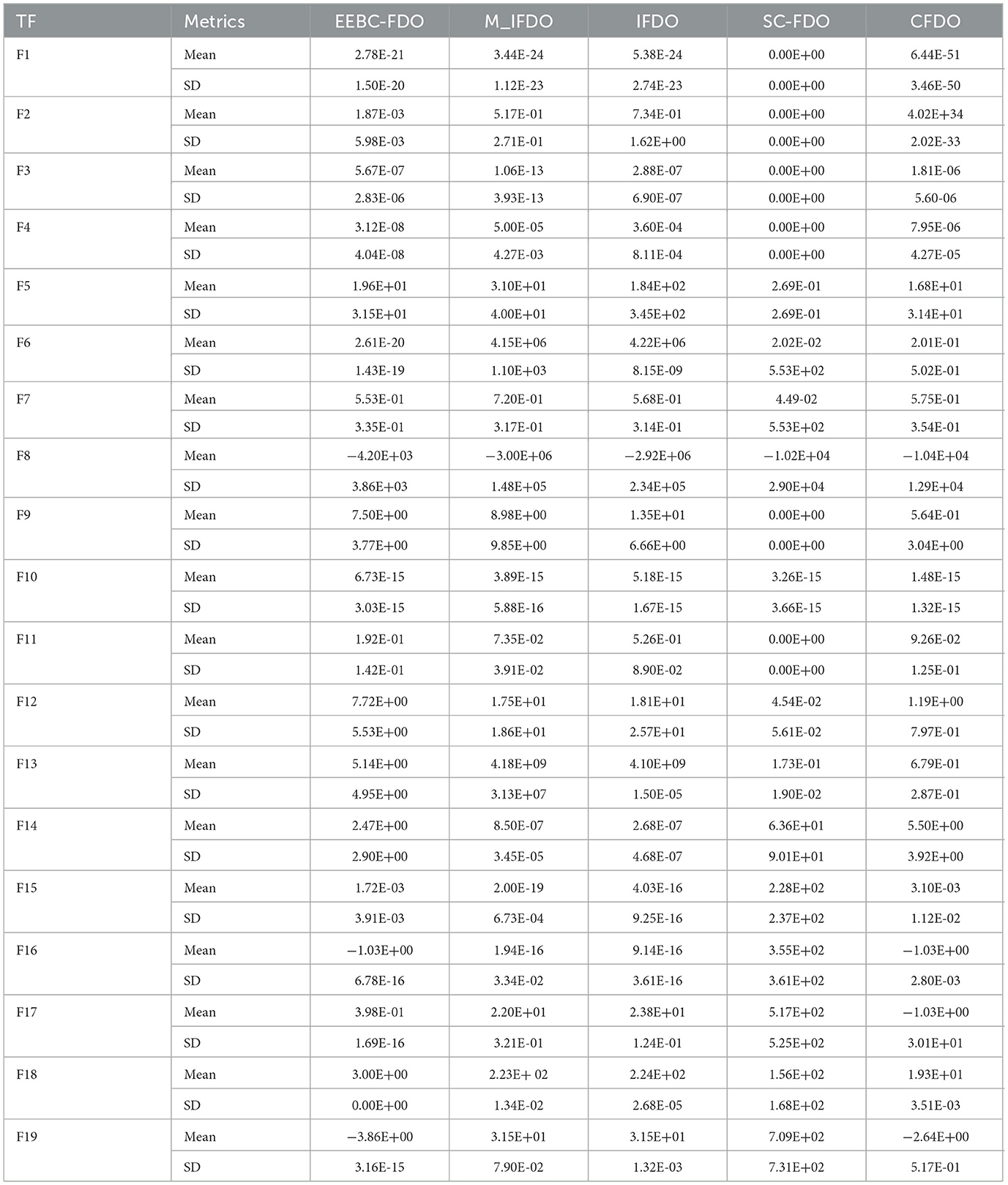
Table 9. Comparing EEBC-FDO with modifications Of FDO using classical benchmark functions.
The use of higher-dimensional evaluations is a critical aspect of validating the effectiveness of EEBC-FDO. To this end, both 20- and 30-dimensional benchmark functions were employed to compare the performance of EEBC-FDO against FDO. In the 20-dimensional case, as shown in Table 10, EEBC-FDO outperformed FDO on functions F1, F4, F6, and F11, while also demonstrating superior average performance on functions F2, F3, F5, F7, F9, F10, and F13. These results confirm the robustness and improved optimization capabilities of EEBC-FDO in more complex, high-dimensional problem spaces. In the second case, using the 30-dimensional benchmark functions, EEBC-FDO exhibited some limitations. While it outperformed FDO on only three functions—F5, F6, and F13—it still achieved better average performance on functions F4, F7, F9, and F10. These results suggest that although EEBC-FDO maintains competitive performance in certain high-dimensional scenarios, its effectiveness may diminish as problem dimensionality increases further.
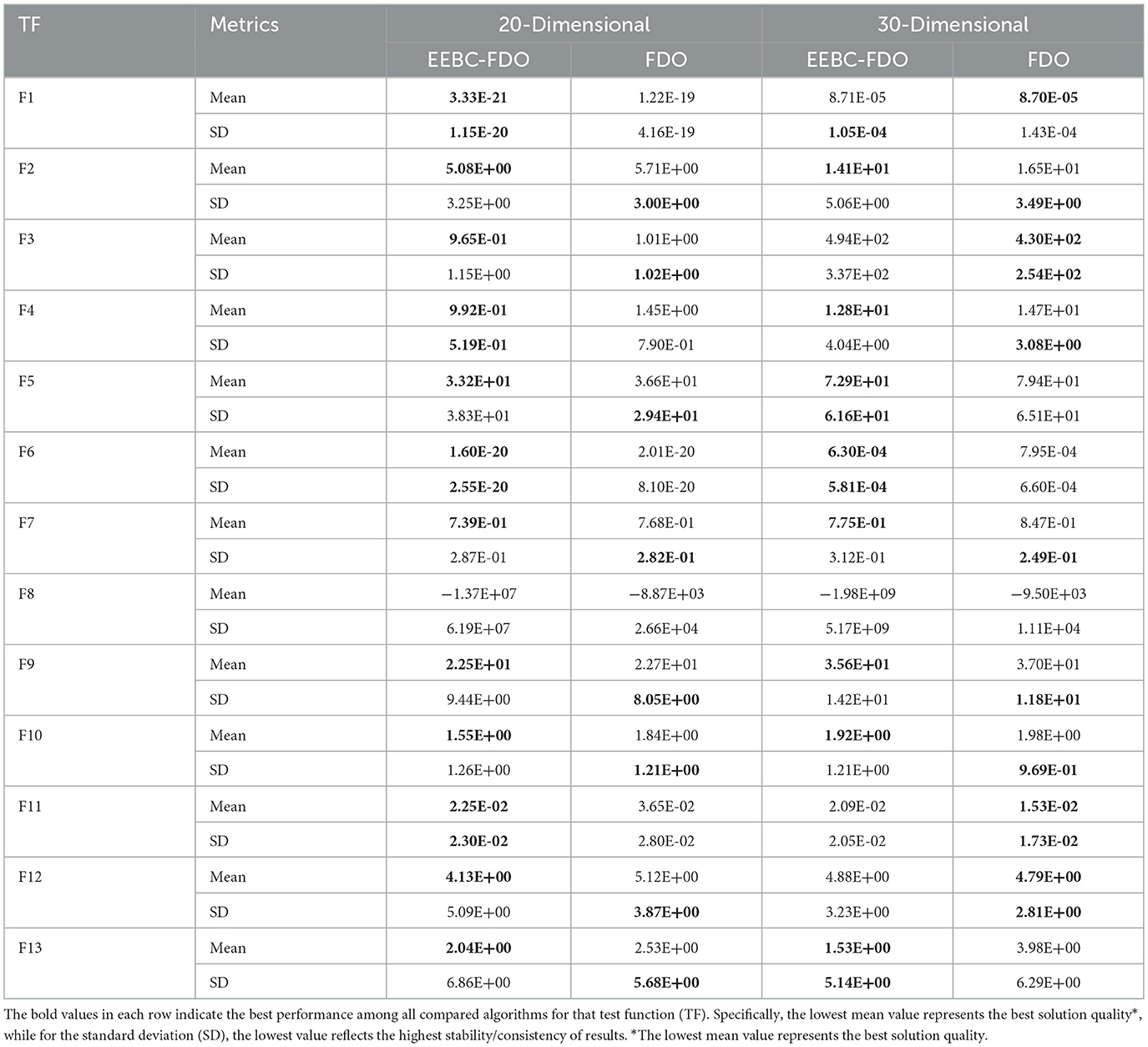
Table 10. Results of comparing EEBC-FDO with FDO for 20- and 30-dimensional algorithms using classical benchmark functions.
6.2 CEC2019 benchmark test functions
Testing EESB-FDO and EEBC-FDO on a single benchmark test function is not a sufficient measure to ensure their effectiveness. Therefore, to thoroughly evaluate their performance and capability, the algorithm was tested on the CEC2019 benchmark functions presented in Table 11, which are commonly used for assessing optimization algorithms. This benchmark set includes ten multimodal test functions, which serve as enhanced evaluation functions for optimization purposes [70].
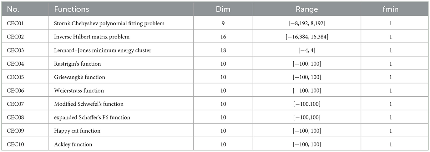
Table 11. CEC-C06 2019 benchmark functions [80].
The results of the proposed EESB-FDO, presented in Table 12, demonstrate its success in outperforming other algorithms, achieving the highest ranking in CEC02, CEC04, CEC05, CEC06, and CEC09. Additionally, in CEC03, CEC08, and CEC10, EESB-FDO obtained the best performance based on the average calculation. Furthermore, the LPB algorithm secured second place and showed competitive performance, particularly in CEC03 and CEC07. Meanwhile, WOA and FOX exhibited similar performance, ranking third overall. Finally, AOA demonstrated the weakest performance among the compared algorithms. On the other hand, Table 13 presents the results of EEBC-FDO, clearly indicating that FDO and EEBC-FDO did not achieve superior performance in the competition, as their results were nearly identical. However, overall, the outcomes demonstrated better performance compared to the other algorithms discussed in this section.
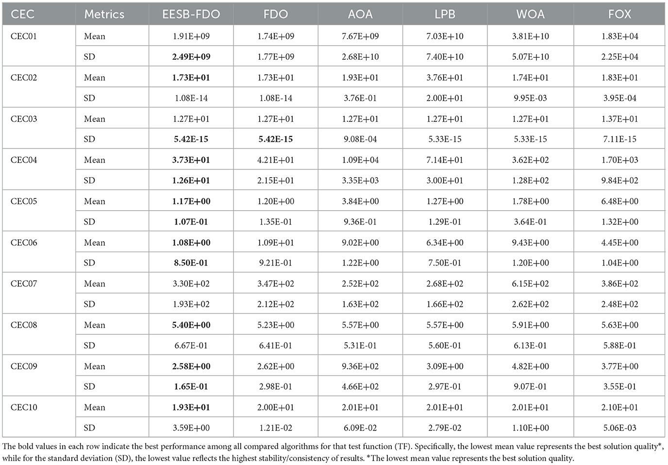
Table 12. Results of comparing EESB-FDO with FDO and other chosen algorithms Using CEC 2019 benchmark functions.
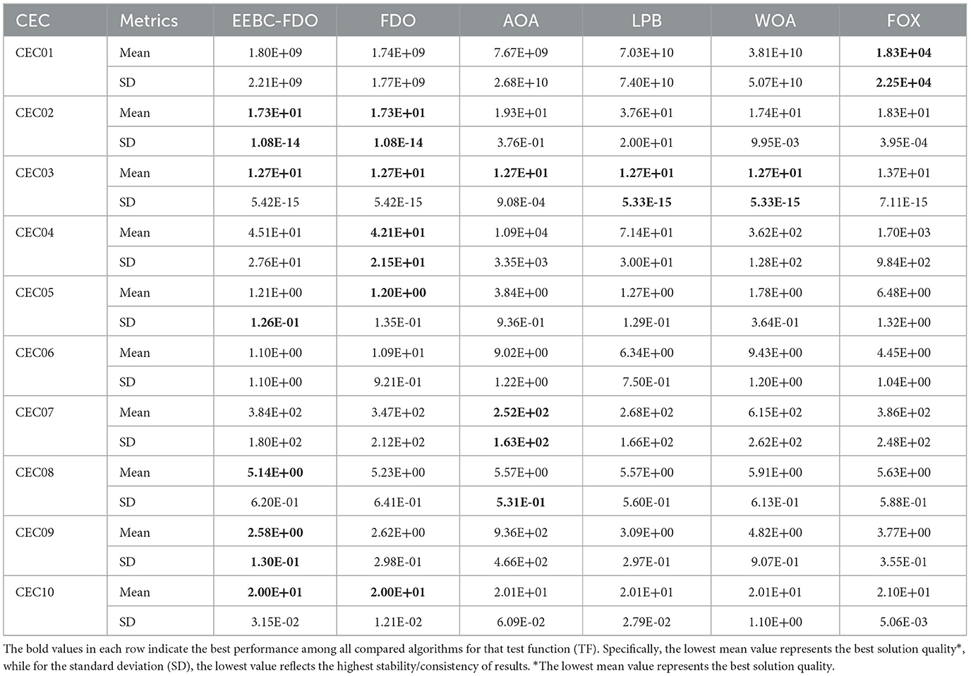
Table 13. Results of comparing EEBC-FDO with FDO and other chosen algorithms using CEC 2019 benchmark functions.
6.3 CEC2022 benchmark test functions
To further evaluate the feasibility of the proposed algorithm, the CEC2022 benchmark test functions were utilized, as presented in Table 14. This benchmark set comprises 12 functions, labeled CEC01 to CEC12, which are organized into four groups: unimodal, multimodal, hybrid, and composite functions. The search space for these benchmark problems is defined within specific ranges of decision variables, constrained within the interval [−100,100] for all test functions. Therefore, d = 10 and 20 dimensions were used to assess the proposed modification [71].
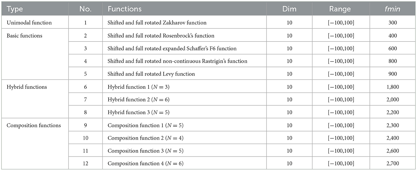
Table 14. CEC-C06 2022 benchmark functions [87].
The results of EESB-FDO, FDO, AOA, LPB, WOA, and FOX were evaluated by d = 10 dimension and are presented in Table 15. The outcomes of the proposed EESB-FDO modification indicate that it achieved the highest rank, outperforming other algorithms in CEC01, CEC02, CEC07, CEC09, and CEC12. Additionally, it obtained the best average performance in CEC05, CEC08, and CEC10. Meanwhile, the LPB algorithm secured second place, demonstrating superior performance in CEC03, CEC04, and CEC06. The FDO ranked third, while the remaining algorithms exhibited the lowest performance. To further evaluate the proposed modifications, Table 16 presents comparative results for both 10- and 20-dimensional problem instances. The outcomes demonstrate that EESB-FDO continues to perform successfully in the 20-dimensional setting, particularly on benchmark functions CEC01, CEC02, CEC05, CEC07, CEC08, CEC11, and CEC12, thereby confirming the robustness and scalability of the algorithm across higher-dimensional search spaces.
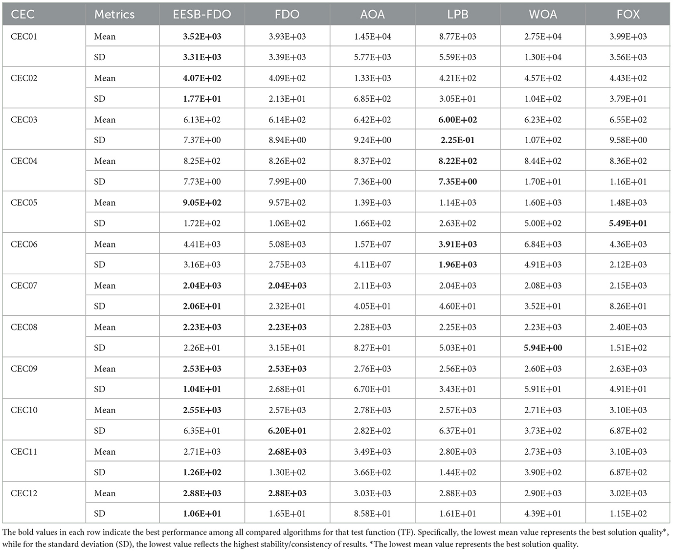
Table 15. Results of comparing EESB-FDO with FDO and Other chosen algorithms using CEC 2022 benchmark functions.
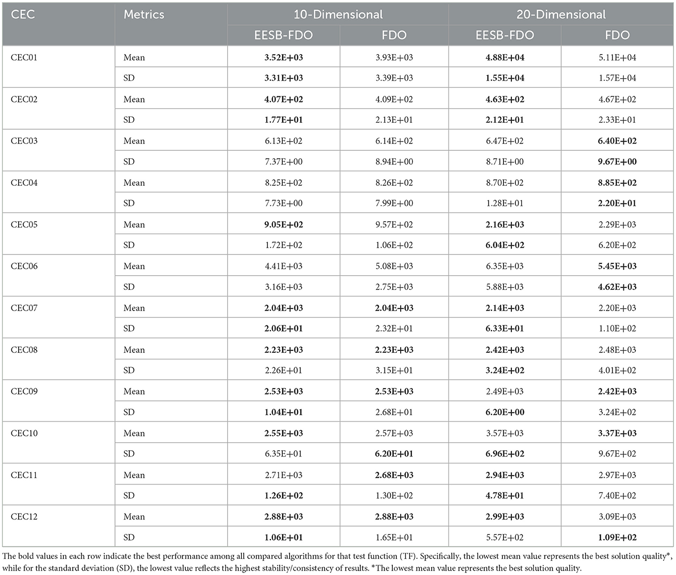
Table 16. Results of comparing EESB-FDO with FDO for 10 and 20 dimensions using CEC 2022 benchmark functions.
On the other hand, as illustrated in Table 17, the results indicate that the EEBC-FDO algorithm outperforms the other algorithms on the CEC03, CEC05, and CEC09 benchmark functions. Conversely, the remaining functions show superior performance by the other algorithms compared to EEBC-FDO. Subsequently, EEBC-FDO was evaluated using 20-dimensional benchmark functions, with the results presented in Table 18. The outcomes indicate that EEBC-FDO achieved superior performance, outperforming all competing algorithms on CEC01, CEC02, CEC06, CEC07, CEC08, and CEC11, thereby demonstrating its effectiveness and competitiveness in high-dimensional optimization tasks.
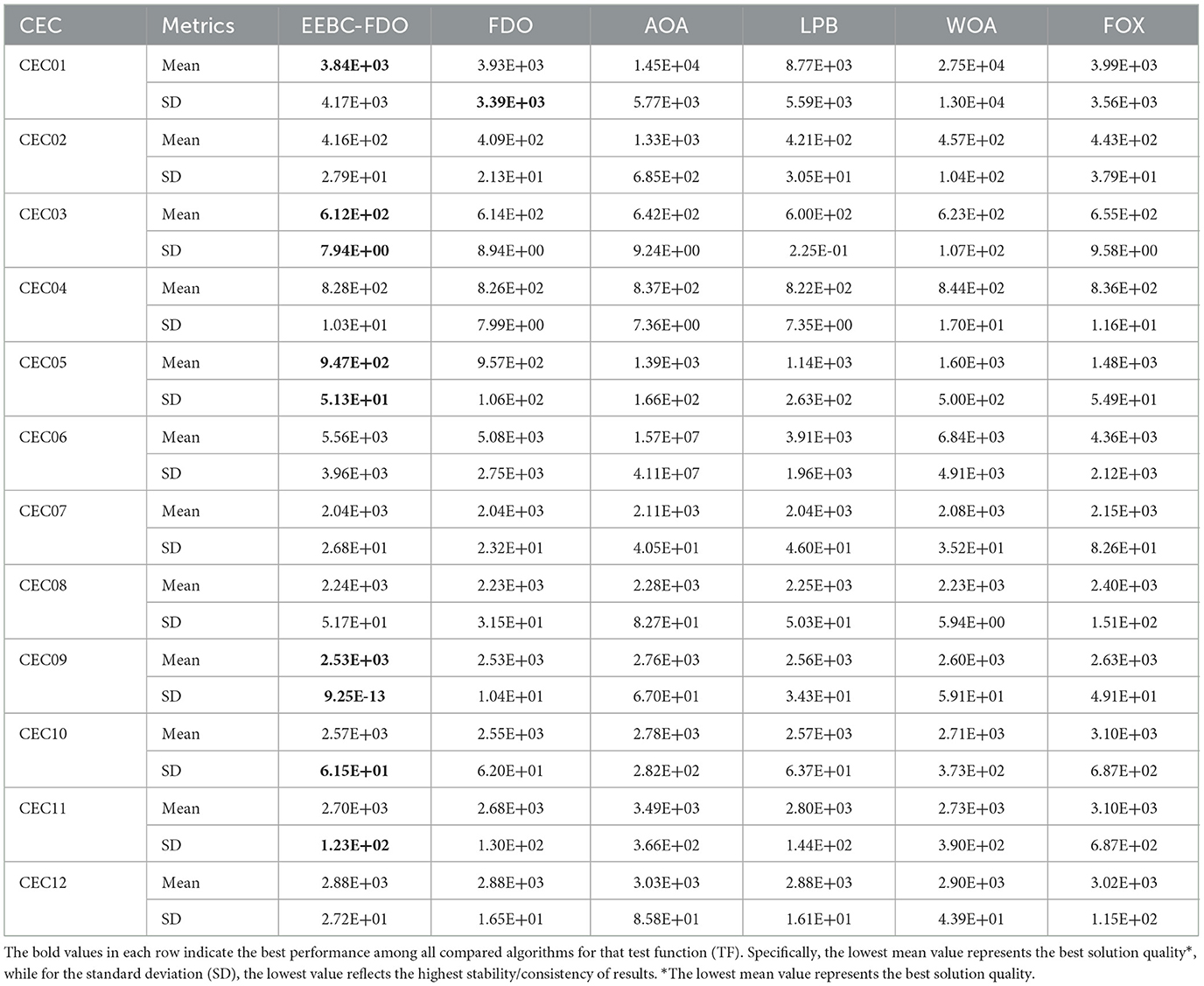
Table 17. Results of comparing EEBC-FDO with FDO and Other chosen algorithms using CEC 2022 benchmark function.
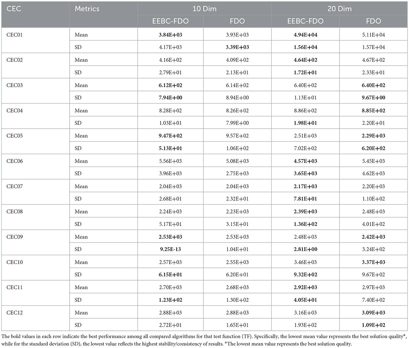
Table 18. Results of comparing EEBC-FDO with FDO for (10 and 20) dimensions using CEC 2022 benchmark function.
6.4 Wilcoxon rank-sum test
One of the primary statistical methods used for hypothesis testing in this study is the Wilcoxon rank-sum test, which evaluates whether the performance differences between two algorithms are statistically significant. This non-parametric test is well-suited for optimization problems, as it does not assume a normal distribution of results and instead relies on rank comparisons. The test produces a p-value (probability value) that quantifies the strength of evidence against the null hypothesis. A smaller p-value (typically p < 0.05) indicates strong evidence to reject the null hypothesis, suggesting that one algorithm significantly outperforms the other, whereas larger p-values imply that the performance difference is not statistically significant [72–74].
Table 19 presents the Wilcoxon test results comparing FDO, EESB-FDO, and EEBC-FDO against MFDO on the CEC2022 benchmark suite. The findings show that, for many functions (e.g., CEC01, CEC03, CEC04, CEC05), the extremely small p-values confirm that the proposed variants achieve statistically significant improvements. In contrast, higher p-values in functions such as CEC02 and CEC09 indicate no significant difference, suggesting that MFDO retains competitiveness in these landscapes, where exploration dominates over exploitation. Notably, EESB-FDO and EEBC-FDO reduce the number of non-significant cases compared to the original FDO, confirming the effectiveness of the proposed modifications in enhancing exploitation and convergence speed. These variations highlight that algorithm performance is problem-dependent: functions requiring stronger exploitation benefit from EESB-FDO and EEBC-FDO, while functions emphasizing broad exploration (e.g., CEC02, CEC09) show less pronounced differences. Overall, the Wilcoxon rank-sum test not only validates the robustness of the proposed variants but also provides insights into the problem characteristics where they achieve the most significant advantages.
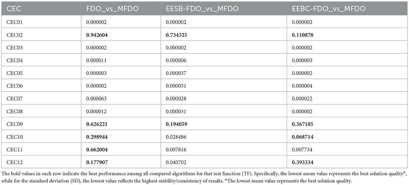
Table 19. WILCOXON rank-sum test for CEC2022 benchmark functions.
6.5 Quantitative measurement metrics
Quantitative analysis is a crucial metric that provides detailed insights and in-depth observations of new algorithms and their modifications. Figures 6–8 illustrate this analysis, where the convergence of iterations represents the measurement of an agent's global best performance. Among the unimodal test functions (TF1–TF7), TF1 was selected as the representative function. For multimodal test functions (TF8–TF13), TF11 was chosen, while for composite test functions (TF14–TF19), TF15 was nominated. To further investigate performance, a two-dimensional search space was explored over 150 iterations using 10 search agents. As the number of iterations increased, (the global best agent) demonstrated greater precision. Additionally, when the scout bee emphasized exploitation and local search, the proposed modifications achieved superior results within fewer iterations, thereby demonstrating the algorithm's adaptability and effectiveness.
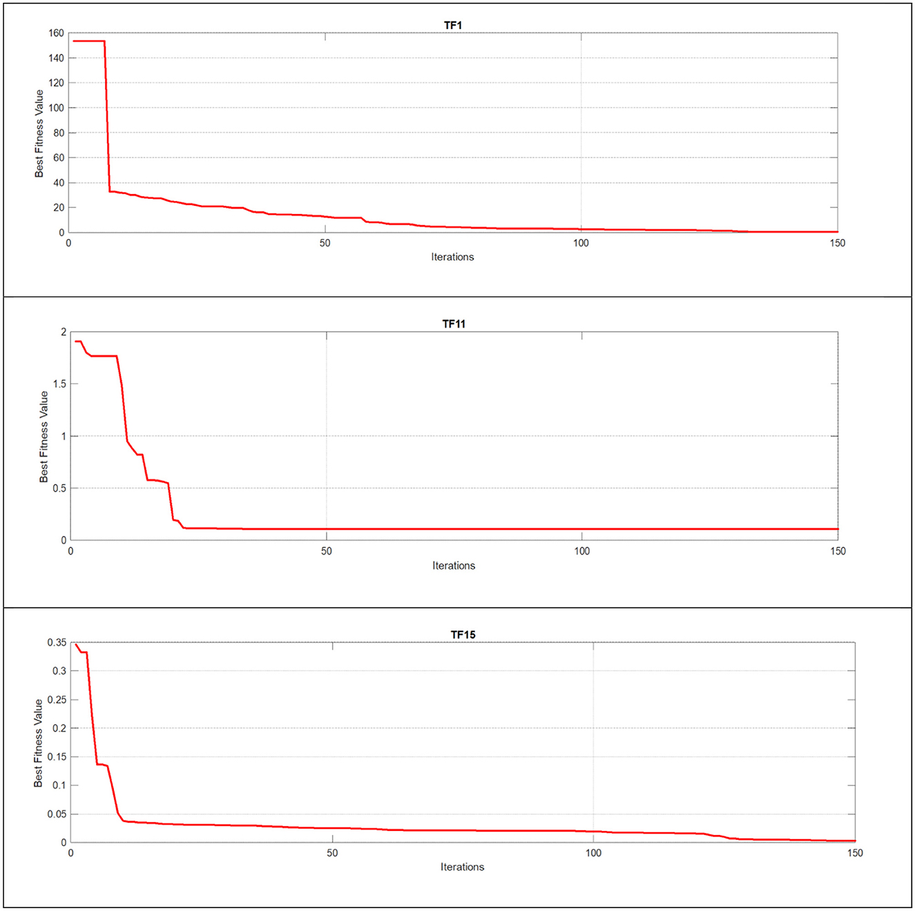
Figure 6. Using unimodal, multimodal, and composite test functions for the FDO algorithm convergence curve.
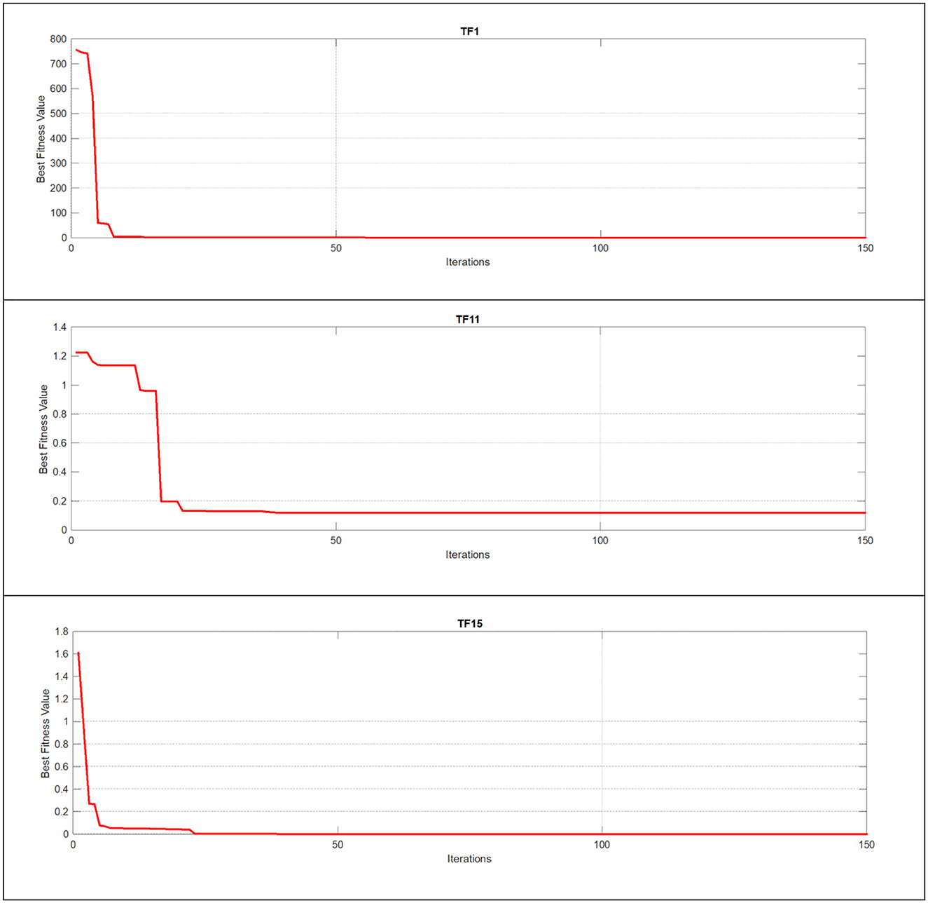
Figure 7. Using unimodal, multimodal, and composite test functions for the EESB-FDO algorithm convergence curve.
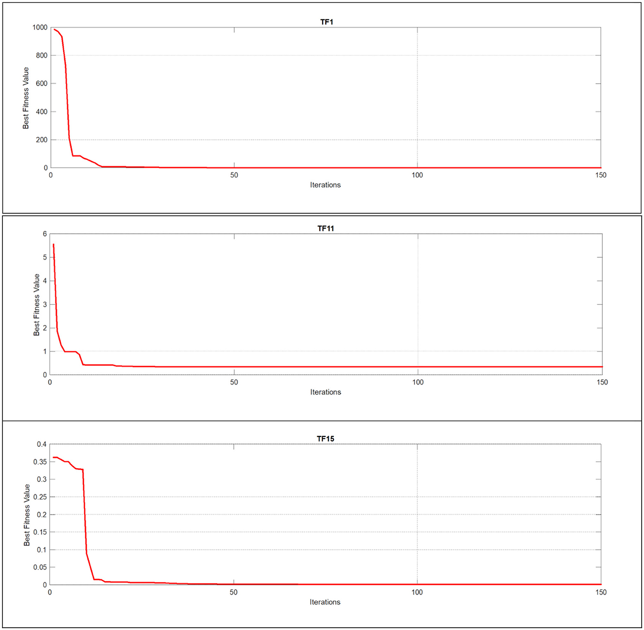
Figure 8. Using unimodal, multimodal, and composite test functions for the EEBC-FDO algorithm convergence curve.
6.6 Real-world applications of EESB-FDO and EEBC-FDO
6.6.1 Gear train design problem
The primary objective of the gear train design (GTD) problem is to minimize the cost associated with the transmission ratio of the gear train configuration illustrated in Figure 9 [75, 76]. This optimization problem involves four discrete decision variables, Ta, Tb,Td, and Tf, each corresponding to the number of teeth on a specific gear within the train. The problem is formulated mathematically as follows:
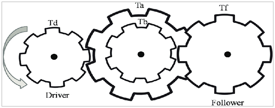
Figure 9. The gear train design problem.
6.6.2 Three-bar truss problem
As illustrated in Figure 10, the three-bar truss structure is considered for structural optimization. The objective is to minimize the total volume of the truss while ensuring that the design adheres to specified stress constraints [77, 78]. The corresponding mathematical formulation is provided below.
where .
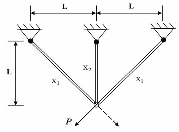
Figure 10. The three-bar truss problem.
6.6.3 The pathological IgG fraction in the nervous system
This real-world problem, described in Ismaeel Ghareb et al. [79], aims to determine the optimal solution for pathological conditions in humans or animals. It is known as the dimmer solution and is used to identify the IgG fraction in the nervous system. The mathematical formulation is presented below.
where Xi represents the input albumin quotient values, and Y(Xi) denotes the corresponding optimized IgG values. These equations, supported by Figure 11, demonstrate a real-world application of statistical modeling and optimization in medical diagnostics, offering an improved framework for evaluating immune dysfunctions in the nervous system.
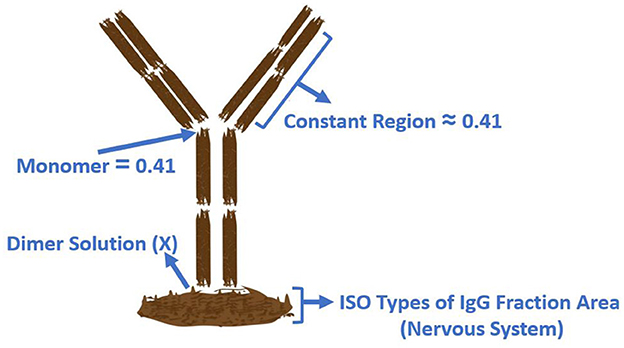
Figure 11. Pathological IgG fraction design problem.
6.6.4 Integrated cyber-physical attack for manufacturing system
This real-world application, supported by Figure 12, is designed to identify potentially harmful nodes within network systems, with a particular focus on software and hardware engineering design phases. The primary objective is to optimize the detection and regulation of these nodes within a normalized range of [0, 1], as their presence can introduce critical vulnerabilities, including system bugs and risk-prone components [80].
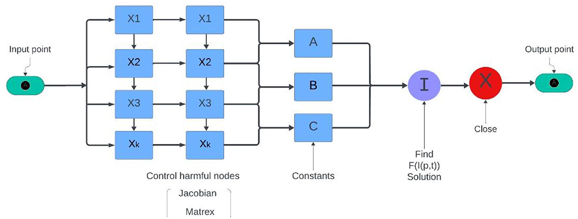
Figure 12. Design problem for a Cyber-physical attack mitigation system.
The fitness function is defined as
where X represents the node state values, and the coefficients A, B, and C are functions of system parameters, calculated as
in these equations, d denotes the total number of nodes (ranging from 15 to 36), while k1∈[0, 1] and k2∈[0.1, 0.5] are system-specific constants reflecting infection rate and risk thresholds. The aim of this fitness function is to identify configurations in which F(I(p, t)) → 0, indicating an optimal system state with minimal harmful node influence.
6.6.5 Real-world application comparison and discussion
The final step in evaluating any newly proposed algorithm or enhancement involves its application to real-world problems. To assess performance, standard evaluation metrics such as the mean, standard deviation, and p-value are employed for comparative analysis. In this section, four real-world applications were utilized to fulfill this objective. The corresponding results are presented in Tables 20–22.
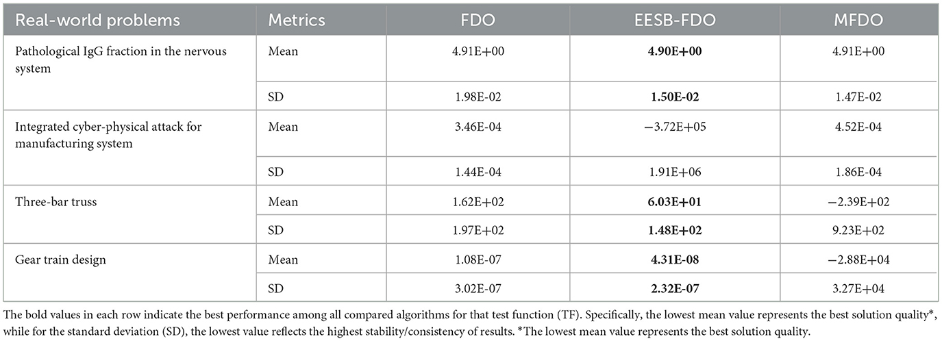
Table 20. The results of comparison FDO with EESB-FDO and MFDO.
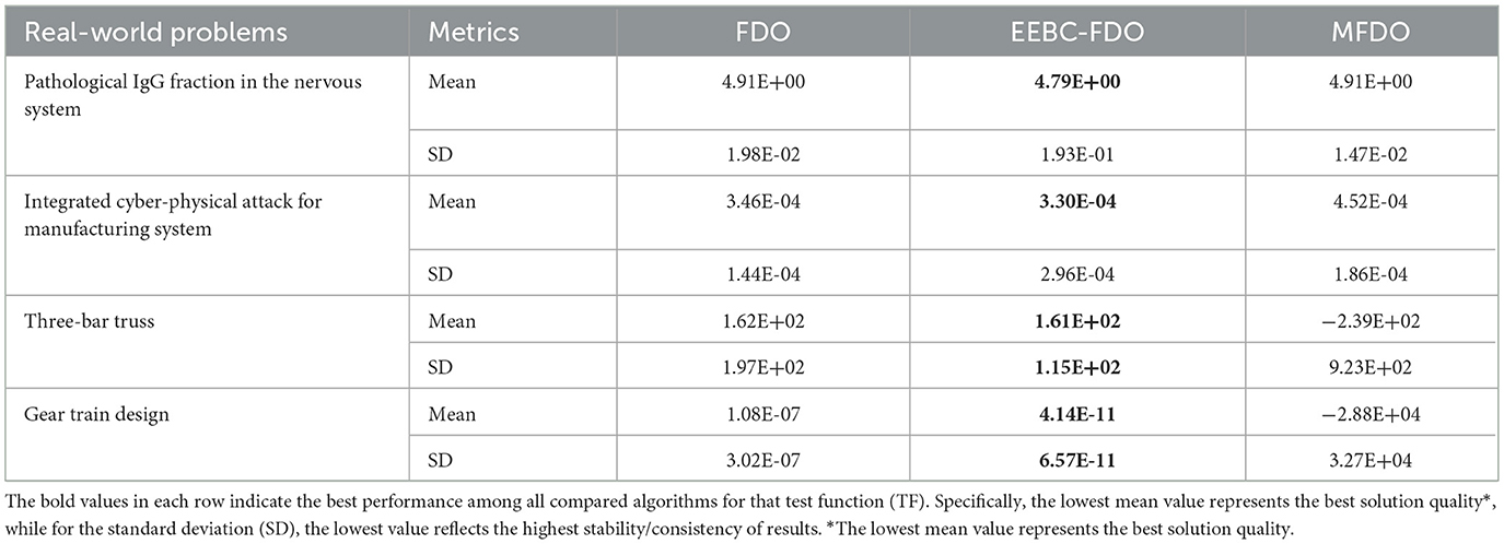
Table 21. The results of comparison FDO with EEBC-FDO and MFDO.
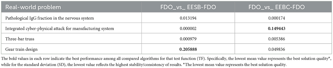
Table 22. WILCOXON rank-sum test for four real-world problems.
The results of EESB-FDO and EEBC-FDO, presented in Tables 20, 21, demonstrate the performance of these two modified versions in comparison with the FDO and MFDO algorithms. In three real-world applications, both EESB-FDO and EEBC-FDO consistently achieved the best rankings, with lower mean and standard deviation values, indicating improved stability and reliability, outperforming the other algorithms. However, one of the modified versions exhibited a slight weakness in a specific case. On the other hand, the p-value, which quantifies the strength of evidence against the null hypothesis, indicates that a smaller p-value, typically p < 0.05, indicates strong evidence to reject the null hypothesis, suggesting that the observed results are unlikely to have occurred by chance. Table 22 shows the results of the comparison between FDO and EESB-FDO, which has just one case that fails to reject the null hypothesis for the gear train design, and FDO with EEBC-FDO, which shows the same result but with a different real-world problem's integrated cyber-physical attack for manufacturing system.
7 Conclusion
This study proposed two enhanced variants of the fitness-dependent optimizer (FDO) designed to address its limitations in exploitation and convergence speed. The first variant, EESB-FDO, introduces a stochastic boundary repositioning mechanism that reassigns scout bees that exceed the search space to random positions within the valid range. The second variant, EEBC-FDO, employs a boundary carving strategy that redirects out-of-bound solutions toward feasible regions using customized correction equations. In addition, a third enhancement, the ELFS strategy, constrains the Levy flight step range to (−1, 1), ensuring more stable and bounded exploration behavior. To validate the effectiveness of these modifications, extensive experiments were conducted using classical benchmark functions and CEC 2019 and CEC 2022 test suites. The results demonstrated that both EESB-FDO and EEBC-FDO significantly improve exploitation capability and convergence performance compared to the FDO and other state-of-the-art algorithms.
In the future, various enhancements and extensions of the current limited work can be developed. An important aspect to improve is the application of multi-objective vector optimization, utilizing functions specifically related to multi-objective optimization techniques [81]. A major limitation of this study lies in the inability to test certain benchmark functions in higher dimensions, which limits the generalizability of the findings. Future work could explore dimensionality reduction techniques or alternative benchmark suites that support high-dimensional testing. While classical benchmark functions can typically be tested across various dimensions, including 50, many CEC2019 functions are restricted and do not support high-dimensional testing. This constraint limits the generalizability and robustness analysis of the proposed algorithm. However, to partially address this issue, the CEC2022 benchmark set, which allows testing with 20 dimensions, can be used as an alternative for future evaluations. Despite these limitations, the enhancements should be applied to classification tasks and parameter tuning to improve the new model. This would also provide an opportunity to test the model on datasets related to education, healthcare, and other fields [79, 82]. Furthermore, the modification of this algorithm has not yet been validated on classification tasks involving real-world healthcare datasets, such as those related to sleep disorders or chronic disease diagnosis [83, 84]. As a result, its adaptability and robustness in managing noisy, imbalanced, and high-dimensional medical data remain uncertain due to the absence of dedicated benchmarking in medical classification scenarios. Although improvements have been demonstrated across several real-world applications, further development is needed by verifying dataset authenticity and incorporating security-focused algorithms to better guide the exploitation and exploration strategies in searching for new solutions [85, 86].
Data availability statement
The original contributions presented in the study are included in the article/supplementary material, further inquiries can be directed to the corresponding author.
Author contributions
AF: Formal analysis, Funding acquisition, Methodology, Writing – original draft, Writing – review & editing, Conceptualization. AMA: Conceptualization, Methodology, Writing – review & editing, Resources. AAA: Conceptualization, Data curation, Writing – review & editing, Project administration.
Funding
The author(s) declare that no financial support was received for the research and/or publication of this article.
Conflict of interest
The authors declare that the research was conducted in the absence of any commercial or financial relationships that could be construed as a potential conflict of interest.
Generative AI statement
The author(s) declare that no Gen AI was used in the creation of this manuscript.
Any alternative text (alt text) provided alongside figures in this article has been generated by Frontiers with the support of artificial intelligence and reasonable efforts have been made to ensure accuracy, including review by the authors wherever possible. If you identify any issues, please contact us.
Publisher's note
All claims expressed in this article are solely those of the authors and do not necessarily represent those of their affiliated organizations, or those of the publisher, the editors and the reviewers. Any product that may be evaluated in this article, or claim that may be made by its manufacturer, is not guaranteed or endorsed by the publisher.
References
1. Sörensen K, Glover F. METAHEURISTICS 1 1 Definition. Available online at: http://metaheuristics.eu (Accessed March 4, 2025).
2. Yang X-S. Nature-Inspired Optimization Algorithms. London: Elsevier (2014). doi: 10.1016/B978-0-12-416743-8.00010-5
3. Fister I, Yang X-S, Fister I, Brest J, Fister D. A Brief Review of Nature-Inspired Algorithms for Optimization (2013). Available online at: http://arxiv.org/abs/1307.4186 (Accessed April 8, 2025).
4. Talbi E. Metaheuristics: From Design to Implementation. Hoboken, NJ: Wiley (2009). doi: 10.1002/9780470496916
5. Mustafa AI, Aladdin AM, Mohammed-Taha SR, Hasan DO, Rashid TA. Is PSO the Ultimate Algorithm or Just Hype? Piscataway, NJ: TechRxiv (2025). doi: 10.36227/techrxiv.173609965.50383071/v1
6. Aladdin AM, Rashid TA. A new Lagrangian problem crossover—a systematic review and meta-analysis of crossover standards. Systems. (2023) 11:144. doi: 10.3390/systems11030144
7. Deb K. An introduction to genetic algorithms. Sadhana. (1999) 24:293–315. doi: 10.1007/BF02823145
8. Hassanat A, Almohammadi K, Alkafaween E, Abunawas E, Hammouri A, Prasath VBS. choosing mutation and crossover ratios for genetic algorithms—a review with a new dynamic approach. Information. (2019) 10:390. doi: 10.3390/info10120390
9. Dokeroglu T, Sevinc E, Kucukyilmaz T, Cosar A. A survey on new generation metaheuristic algorithms. Comput Ind Eng. (2019) 137:106040. doi: 10.1016/j.cie.2019.106040
10. Kennedy J, Eberhart R. Particle swarm optimization. In: Proceedings of ICNN'95 - International Conference on Neural Networks. IEEE, p. 1942–8. doi: 10.1109/ICNN.1995.488968
11. Yapici H, Cetinkaya N. A new meta-heuristic optimizer: pathfinder algorithm. Appl Soft Comput J. (2019) 78:545–68. doi: 10.1016/j.asoc.2019.03.012
12. Zervoudakis K, Tsafarakis S. A mayfly optimization algorithm. Comput Ind Eng. (2020) 145:106559. doi: 10.1016/j.cie.2020.106559
13. Ghasemi-Marzbali A. A novel nature-inspired meta-heuristic algorithm for optimization: bear smell search algorithm. Soft comput. (2020) 24:13003–35,. doi: 10.1007/s00500-020-04721-1
14. Ahmadianfar I, Bozorg-Haddad O, Chu X. Gradient-based optimizer: a new metaheuristic optimization algorithm. Inf Sci (N Y). (2020) 540:131–59. doi: 10.1016/j.ins.2020.06.037
15. Zhang Y, Jin Z. Group teaching optimization algorithm: a novel metaheuristic method for solving global optimization problems. Expert Syst Appl. (2020) 148:113246. doi: 10.1016/j.eswa.2020.113246
16. Askari Q, Saeed M, Younas I. Heap-based optimizer inspired by corporate rank hierarchy for global optimization. Expert Syst Appl. (2020) 161:113702. doi: 10.1016/j.eswa.2020.113702
17. Hashim FA, Houssein EH, Mabrouk MS, Al-Atabany W, Mirjalili S. Henry gas solubility optimization: a novel physics-based algorithm. Fut Gen Comput Syst. (2019) 101:646–67. doi: 10.1016/j.future.2019.07.015
18. Faramarzi A, Heidarinejad M, Mirjalili S, Gandomi AH. Marine Predators Algorithm: A Nature-inspired Metaheuristic. Available online at: https://linkinghub.elsevier.com/retrieve/pii/S0957417420302025
19. Askari Q, Younas I, Saeed M. Political optimizer: a novel socio-inspired meta-heuristic for global optimization. Knowl Based Syst. (2020) 195:105709. doi: 10.1016/j.knosys.2020.105709
20. Zhao W, Wang L, Zhang Z. Atom search optimization and its application to solve a hydrogeologic parameter estimation problem. Knowl Based Syst. (2019) 163:283–304. doi: 10.1016/j.knosys.2018.08.030
21. Abualigah L, Yousri D, Abd Elaziz M, Ewees AA, Al-qaness MAA, Gandomi AH. Aquila Optimizer: a novel meta-heuristic optimization algorithm. Comput Ind Eng. (2021) 157:107250. doi: 10.1016/j.cie.2021.107250
22. MiarNaeimi F, Azizyan G, Rashki M. Horse herd optimization algorithm: a nature-inspired algorithm for high-dimensional optimization problems. Knowl Based Syst. (2021) 213:106711. doi: 10.1016/j.knosys.2020.106711
23. Oyelade ON, Ezugwu AES, Mohamed TIA, Abualigah L. Ebola optimization search algorithm: a new nature-inspired metaheuristic optimization algorithm. IEEE Access. (2022) 10:16150–77. doi: 10.1109/ACCESS.2022.3147821
24. Shami TM, Grace D, Burr A, Mitchell PD. Single candidate optimizer: a novel optimization algorithm. Evol Intell. (2024) 17:863–87. doi: 10.1007/s12065-022-00762-7
25. Wolpert DH, Macready WG. No free lunch theorems for optimization. IEEE Trans Evol Comput. (1997) 1:67–82. doi: 10.1109/4235.585893
26. Arora S, Singh S. A conceptual comparison of firefly algorithm, bat algorithm and cuckoo search in 2013. In: International Conference on Control, Computing, Communication and Materials (ICCCCM). Allahabad: IEEE (2013). p. 1–4. doi: 10.1109/ICCCCM.2013.6648902
27. Cohen JD, McClure SM, Yu AJ. Should I stay or should I go? How the human brain manages the trade-off between exploitation and exploration. Philos Trans R Soc B: Biol Sci. (2007) 2007:933–42. doi: 10.1098/rstb.2007.2098
28. Mehlhorn K, Newell BR, Todd PM, Lee MD, Morgan K, Braithwaitt VA, et al. Unpacking the exploration-exploitation tradeoff: a synthesis of human and animal literatures. Decision. (2015) 2:191–215. doi: 10.1037/dec0000033
29. March JG Exploration and exploitation in organizational learning. Organiz Sci. (1991) 2:71–87. doi: 10.1287/orsc.2.1.71
30. Aladdin M, Abdullah JM, Salih KOM, Rashid TA, Sagban R, Alsaddon A, et al. Fitness dependent optimizer for IoT healthcare using adapted parameters: a case study implementation. In: Practical Artificial Intelligence for Internet of Medical Things. Boca Raton, FL: CRC Press (2023). 45–61. doi: 10.1201/9781003315476-3
31. Abdullah JM, Ahmed T. Fitness dependent optimizer: inspired by the bee swarming reproductive process. IEEE Access. (2019) 7:43473–86. doi: 10.1109/ACCESS.2019.2907012
32. Muhammed DA, Saeed SAM, Rashid TA. Improved fitness-dependent optimizer algorithm. IEEE Access. (2020) 8:19074–88. doi: 10.1109/ACCESS.2020.2968064
33. Chiu PC, Selamat A, Krejcar O, Kuok KK. Hybrid sine cosine and fitness dependent optimizer for global optimization. IEEE Access. (2021) 9:128601–22. doi: 10.1109/ACCESS.2021.3111033
34. Salih JF, Mohammed HM, Abdul ZK. Modified fitness dependent optimizer for solving numerical optimization functions. IEEE Access. (2022) 10:83916–30. doi: 10.1109/ACCESS.2022.3197290
35. Abdulla HS, Ameen AA, Saeed SI, Mohammed IA, Rashid TA. MRSO: balancing exploration and exploitation through modified rat swarm optimization for global optimization. Algorithms. (2024) 17:423. doi: 10.3390/a17090423
37. Srinivas M, Patnaik LM. Adaptive probabilities of crossover and mutation in genetic algorithms. IEEE Trans Syst Man Cybern. (1994) 24:656–67. doi: 10.1109/21.286385
38. Liang JJ, Qin AK, Suganthan PN, Baskar S. Comprehensive learning particle swarm optimizer for global optimization of multimodal functions. IEEE Trans Evol Comput. (2006) 10:281–95. doi: 10.1109/TEVC.2005.857610
39. Blum C. Ant colony optimization: introduction and recent trends. Phys Life Rev. (2005) 2:353–73. doi: 10.1016/j.plrev.2005.10.001
40. Stützle T, Hoos HH. Ant system. Fut Gen Comput Syst. (2000) 16:889–914. doi: 10.1016/S0167-739X(00)00043-1
41. Cheung NJ, Ding X-M, Shen H-B. Adaptive firefly algorithm: parameter analysis and its application. PLoS ONE. (2014) 9:e112634. doi: 10.1371/journal.pone.0112634
42. Abualigah L, Diabat A, Mirjalili S, Abd Elaziz M, Gandomi AH. The arithmetic optimization algorithm. Comput Methods Appl Mech Eng. (2021) 376:113609. doi: 10.1016/j.cma.2020.113609
43. Zhang J, Zhang G, Huang Y, Kong M. A novel enhanced arithmetic optimization algorithm for global optimization. IEEE Access. (2022) 10:75040–62. doi: 10.1109/ACCESS.2022.3190481
44. Bhattacharyya T, Chatterjee B, Singh PK, Yoon JH, Geem ZW, Sarkar R. Mayfly in harmony: a new hybrid meta-heuristic feature selection algorithm. IEEE Access. (2020) 8:195929–45. doi: 10.1109/ACCESS.2020.3031718
45. Mohammed HM, Rashid TA. Chaotic fitness-dependent optimizer for planning and engineering design. Soft Comput. (2021) 25:14281–95. doi: 10.1007/s00500-021-06135-z
46. Abdul-Minaam DS, Al-Mutairi MES W, Awad MA, El-Ashmawi WH. An adaptive fitness-dependent optimizer for the one-dimensional bin packing problem. IEEE Access. (2020) 8:97959–74. doi: 10.1109/ACCESS.2020.2985752
47. Daraz A, Malik SA, Mokhlis H, Haq IU, Laghari GF, Mansor NN. Fitness dependent optimizer-based automatic generation control of multi-source interconnected power system with non-linearities. IEEE Access. (2020) 8:100989–1003. doi: 10.1109/ACCESS.2020.2998127
48. Daraz A, Malik SA, Mokhlis H, Haq IU, Zafar F, Mansor NN. Improved-fitness dependent optimizer based FOI-PD controller for automatic generation control of multi-source interconnected power system in deregulated environment. IEEE Access. (2020) 8:197757–75. doi: 10.1109/ACCESS.2020.3033983
49. Daraz A, Abdullah Malik S, Haq IU, Khan KB, Laghari GF, Zafar F. Modified PID controller for automatic generation control of multi-source interconnected power system using fitness dependent optimizer algorithm. PLoS ONE. (2020) 15:e0242428. doi: 10.1371/journal.pone.0242428
50. Abbas DK, Rashid TA, Abdalla KH, Bacanin N, Alsadoon A. Using fitness dependent optimizer for training multi-layer perceptron. J Internet Technol. (2021) 22:1575–85. doi: 10.53106/160792642021122207011
51. Laghari GF, Malik SA, Daraz A, Ullah A, Alkhalifah T, Aslam S. A numerical approach for solving nonlinear optimal control problems using the hybrid scheme of fitness dependent optimizer and bernstein polynomials. IEEE Access. (2022) 10:50298–313. doi: 10.1109/ACCESS.2022.3173285
52. Mirza F, Haider SK, Ahmed A, Rehman AU, Shafiq M, Bajaj M, et al. Generalized regression neural network and fitness dependent optimization: application to energy harvesting of centralized TEG systems. Energy Rep. (2022) 8:6332–46. doi: 10.1016/j.egyr.2022.05.003
53. Tahir H, Rashid TA, Rauf HT, Bacanin N, Chhabra M, Vimal S, et al. Improved Fitness-Dependent Optimizer for Solving Economic Load Dispatch Problem. London: Hindawi Limited (2022). doi: 10.1155/2022/7055910
54. Abdulkhaleq MT, Rashid TA, Hassan BA, Alsadoon A, Bacanin N, Chhabra A, et al. Fitness dependent optimizer with neural networks for COVID-19 patients. Comput Methods Programs Biomed. (2023). 3:100090. doi: 10.1016/j.cmpbup.2022.100090
55. Rathi S, Nagpal R, Srivastava G, Mehrotra D. A multi-objective fitness dependent optimizer for workflow scheduling. Appl Soft Comput. (2024) 152:111247. doi: 10.1016/j.asoc.2024.111247
56. El-Ashmawi WH, Slowik A, Ali AF. An effective fitness dependent optimizer algorithm for edge server allocation in mobile computing. Soft Comput. (2024) 28:6855–77. doi: 10.1007/s00500-023-09582-y
57. Farahmand-Tabar S, Rashid TA. Steel plate fault detection using the fitness dependent optimizer and neural networks. arXiv [Preprint]. arXiv:2405.00006. (2024). doi: 10.48550/arXiv.2405.00006
58. Roy S, Sinha Chaudhuri S. Cuckoo search algorithm using lèvy flight: a review. Int J Modern Educ Comput Sci. (2013) 5:10–5. doi: 10.5815/ijmecs.2013.12.02
59. Yang X-S. Flower pollination algorithm for global optimization. In:Durand-Lose J, Jonoska N, , editors. Unconventional Computation and Natural Computation. Vol. 7445. London: Springer (2012). 240-9. doi: 10.1007/978-3-642-32894-7_27
60. Mirjalili S. Dragonfly algorithm: a new meta-heuristic optimization technique for solving single-objective, discrete, and multi-objective problems. Neural Comput Appl. (2016) 27:1053–73. doi: 10.1007/s00521-015-1920-1
61. Qin F, Zain AM, Zhou K-Q, Yusup NB, Prasetya DD, Abdul R. Hybrid harmony search algorithm integrating differential evolution and Lévy flight for engineering optimization. IEEE Access. (2025) 13:13534–72. doi: 10.1109/ACCESS.2025.3529714
62. Mirjalili S, Gandomi AH, Mirjalili SZ, Saremi S, Faris H, Mirjalili SM. Salp Swarm algorithm: a bio-inspired optimizer for engineering design problems. Adv Eng Softw. (2017) 114:163–91. doi: 10.1016/j.advengsoft.2017.07.002
63. Li S, Chen H, Wang M, Heidari AA, Mirjalili S. Slime mould algorithm: a new method for stochastic optimization. Fut Gen Comput Syst. (2020) 111:300–23. doi: 10.1016/j.future.2020.03.055
64. Xie J, Zhou Y, Chen H. A Novel Bat Algorithm based on differential operator and Lévy flights trajectory. Comput Intell Neurosci. (2013) 2013:1–13. doi: 10.1155/2013/453812
65. Mirjalili S, Mirjalili SM, Lewis A. Grey Wolf optimizer. Adv Eng Softw. (2014) 69:46–61. doi: 10.1016/j.advengsoft.2013.12.007
66. Rashedi E, Nezamabadi-pour H, Saryazdi S. GSA: a gravitational search algorithm. Inf Sci (N Y). (2009) 179:2232–48. doi: 10.1016/j.ins.2009.03.004
67. Rahman CM, Rashid TA. A new evolutionary algorithm: learner performance based behavior algorithm. Egypt Inform J. (2021) 22:213–23. doi: 10.1016/j.eij.2020.08.003
68. Mirjalili S, Lewis A. The Whale optimization algorithm. Adv Eng Softw. (2016) 95:51–67. doi: 10.1016/j.advengsoft.2016.01.008
69. Mohammed HM, Rashid TA. Applied Intelligence. London: Springer (2022). doi: 10.21203/rs.3.rs-1939478/v1
70. Price KV, Awad NH, Ali MZ, Suganthan PN. Problem de- nitions and Evaluation Criteria for the 100-Digit Challenge Special Session and Competition on Single Objective Numerical Optimization. Nanyang Technol. Univ. Singapore, Singapore, Tech. Rep. (2018).
71. Ahrari A, Elsayed SM, Sarker R, Essam D, Coello CAC. Problem Definitions and Evaluation Criteria for the CEC 2022 Special Session and Competition on Single Objective Bound Constrained Numerical Optimization. Canberra, ACT: University of New South Wales (2022).
72. de Barros RSM, Hidalgo JIG, de Cabral DRL. Wilcoxon rank sum test drift detector. Neurocomputing. (2018) 275:1954–63. doi: 10.1016/j.neucom.2017.10.051
73. Thiese MS, Ronna B, Ott U. P value interpretations and considerations. J Thorac Dis. (2016) 8:E928–31. doi: 10.21037/jtd.2016.08.16
74. Amin AAH, Aladdin AM, Hasan DO, Mohammed-Taha SR, Rashid TA. Enhancing algorithm selection through comprehensive performance evaluation: statistical analysis of stochastic algorithms. Computation. (2023) 11:231. doi: 10.3390/computation11110231
75. Bidar M, Mouhoub M, Sadaoui S, Kanan HR. A novel nature-inspired technique based on mushroom reproduction for constraint solving and optimization. Int J Comput Intell Appl. (2020) 19:108. doi: 10.1142/S1469026820500108
76. EKER E. Performance evaluation of capuchin search algorithm through non-linear problems, and optimization of gear train design problem. Eur J Technic. (2023) 13:142–9. doi: 10.36222/ejt.1391524
77. Ray T, Saini P. Engineering design optimization using a swarm with an intelligent information sharing among individuals. Eng Optimiz. (2001) 33:735–748. doi: 10.1080/03052150108940941
78. Fauzi H, Batool U. A Three-bar Truss Design using single-solution simulated Kalman filter optimizer. Mekatronika. (2019) 1:98–102. doi: 10.15282/mekatronika.v1i2.4991
79. Ismaeel Ghareb M, Ali Ahmed Z, Abdullah Ameen A. planning strategy and the use of information technology in higher education: a review study in Kurdistan region government. Int J Inform Visualiz. (2019) 3:283–7. doi: 10.30630/joiv.3.3.263
80. Aladdin AM, Rashid TA. Leo: Lagrange Elementary Optimization. Neural Comput Appl.(2025). 37:14365–97. doi: 10.1007/s00521-025-11225-2
81. Rashid TA, Ahmed AM, Hassan BA, Yaseen ZM, Mirjalili S, Bacanin N, et al. Multi-Objective Optimization Techniques. CRC Press (2025).
82. Hasan DO, Aladdin AM, Hama Amin AA, Rashid TA, Ali YH, Al-Bahri M, et al. Perspectives on the impact of e-learning pre- and post-COVID-19 pandemic—the case of the Kurdistan Region of Iraq. Sustainability. (2023) 15:4400. doi: 10.3390/su15054400
83. Mohammed-Taha SR, Aladdin AM, Mustafa AI, Hasan DO, Muhammed RK, Rashid TA. Analyzing the impact of the pandemic on insomnia prediction using machine learning classifiers across demographic groups. Netw Model Anal Health Inform Bioinform. (2025) 14:51. doi: 10.1007/s13721-025-00552-y
84. Hasan DO, Aladdin AM. Sleep-related consequences of the COVID-19 pandemic: a survey study on insomnia and sleep apnea among affected individuals. Insights Public Health J. (2025) 5:12972. doi: 10.20884/1.iphj.2024.5.2.12972
85. Abdulla HS, Aladdin AM. Enhancing design and authentication performance model: a multilevel secure database management system. Fut Internet. (2025) 17:74. doi: 10.3390/fi17020074
86. Muhammed RK, et al. Comparative analysis of AES, Blowfish, Twofish, Salsa20, and ChaCha20 for image encryption. Kurdistan J Appl Res. (2024) 9:52–65. doi: 10.24017/science.2024.1.5
87. Hasan DO, Mohammed HM, Abdul ZK. Griffon vultures optimization algorithm for solving optimization problems. Expert Syst Appl. (2025) 276:127206. doi: 10.1016/j.eswa.2025.127206
Appendix
This appendix provides a detailed of the benchmark test functions employed to assess the performance of the proposed algorithms. The evaluation includes a comprehensive set of functions categorized into three main groups: classical benchmark functions (unimodal, multimodal, and composite types), as well as the CEC 2019 and CEC 2022 benchmark suites.
Keywords: stochastic boundary, optimization, fitness dependent optimizer, metaheuristic algorithm, Levy flight
Citation: Faraj AK, Aladdin AM and Ameen AA (2025) EESB-FDO: enhancing the fitness-dependent optimizer through a modified boundary handling mechanism. Front. Appl. Math. Stat. 11:1640044. doi: 10.3389/fams.2025.1640044
Received: 03 June 2025; Accepted: 17 September 2025;
Published: 17 October 2025.
Edited by:
Betül Yildiz, Bursa Uludag Universitesi, TürkiyeReviewed by:
Zakariya Yahya Algamal, University of Mosul, IraqLucas Wekesa, Strathmore University Institute of Mathematical Sciences, Kenya
Copyright © 2025 Faraj, Aladdin and Ameen. This is an open-access article distributed under the terms of the Creative Commons Attribution License (CC BY). The use, distribution or reproduction in other forums is permitted, provided the original author(s) and the copyright owner(s) are credited and that the original publication in this journal is cited, in accordance with accepted academic practice. No use, distribution or reproduction is permitted which does not comply with these terms.
*Correspondence: Aram Kamal Faraj, YXJhbS5rYW1hbEBzcHUuZWR1Lmlx; Aso M. Aladdin, YXNvLmFsYWRkaW5AY2h1LmVkdS5pcQ==
†Present address: Aso M. Aladdin Department of Computer Engineering, Tishk International University, Erbil, KR, Iraq
‡ORCID: Aso M. Aladdin orcid.org/0000-0002-8734-0811