Research on error control method for polynomial approximation based on equal amplitude oscillation theorem

To address the issue that polynomial approximation methods strongly depend on the analytical form of the objective function, this study proposes a new minimax polynomial approximation method based on the Chebyshev equioscillation theorem. It constructs near-optimal solutions through discrete sample points, introduces a threshold relaxation strategy to locate equioscillation points, and establishes a coefficient solution framework based on linear equations. Experiments cover both noiseless and noisy data scenarios. Compared with methods such as the Least Squares Method (LSM), the results show that the maximum absolute error of the proposed method is effectively reduced, and it performs excellently under different data densities and distributions. This can provide theoretical support for extreme deviation suppression in engineering fields, especially in safety-critical systems.

Highlights

• Develop a minimax polynomial approximation method based on Chebyshev's theorem for discrete data.

• Introduce a threshold relaxation strategy and linear equation - based coefficient solving for discrete approximation.

• Significantly reduce the maximum absolute error compared to traditional methods, suitable for engineering error control.

1 Introduction

In existing research in the field of polynomial approximation, a research team from Stanford University, USA (1), based on the reproducing kernel Hilbert space theory in functional analysis, proposed a discrete data polynomial approximation framework. By constructing specific reproducing kernel functions, discrete sample points are mapped to a high-dimensional feature space, enabling optimal approximation of functions in the high-dimensional space. This breaks through the limitations of traditional polynomial approximation in terms of discrete data dimension and complexity, providing new ideas for solving approximation problems of high-dimensional discrete data, but the actual application and deployment cost is high. Meanwhile, scholars from the Technical University of Munich, Germany (2), aiming at the discrete minimax approximation problem, proposed an algorithm based on dynamic programming. By orderly partitioning discrete point sets and solving them step by step, the time and space complexity of the algorithm are effectively reduced, enabling rapid processing of large-scale discrete data. A research team from Peking University (3) conducted in-depth research on the equioscillation characteristics of discrete point sets. By introducing the concept of discrete norm, they discretized and transformed the traditional equioscillation theorem, making it suitable for discrete data scenarios. They proposed a judgment criterion for discrete equioscillation points, which comprehensively considers the distribution characteristics of sample points and the change trend of function values, and can effectively construct minimax approximation polynomials based on discrete data. A research group from Tsinghua University (4), aiming at the problem that the traditional Remez algorithm is prone to fall into local optimal solutions in discrete scenarios, introduced a random perturbation mechanism and an adaptive step size adjustment strategy, which effectively avoided the premature convergence of the algorithm. Combining the ideas of intelligent optimization algorithms, they designed a hybrid iterative algorithm, improving the efficiency and accuracy of the algorithm in searching for optimal polynomials in discrete data.

It can be concluded that there are still urgent problems to be solved in the research on discrete data in the field of polynomial approximation. A unified and perfect system for the optimality theory of polynomial approximation under discrete data has not yet been formed. Research on the compatibility and complementarity between different theoretical methods needs to be strengthened. Traditional minimax methods are difficult to apply directly because they require complete function information. The lack of a theoretical system leads to a lack of unified guidance for method design in discrete scenarios. Therefore, constructing a minimax approximation method based on discrete sample points, which has both theoretical rigor and engineering practicability, can provide theoretical support for error control strategies in engineering fields.

2 Discrete approximation method based on equal amplitude oscillation theorem

Given a discrete sample point set $D={\left\{\right(x_i,y_i\left)\right\}}_{i=1}^N$ of an unknown continuous function $f\left(x\right)\in$ C [a, b], where x_i ∈ [a, b]_, y_i = f (x_i) + δ_i, δ_i is observation noise, this study can construct an nth-degree polynomial $p_n\left(x\right)$ $\in {\mathbb{P}}_n$ , ${\mathbb{P}}_n$ represents the space of polynomials of degree ≤n, minimize the maximum absolute error on the discrete point set:

$\underset{p_n\in {\mathbb{P}}_n}{min}\underset{(x_i,y_i)\in D}{max}\mid y_i-p_n\left(x_i\right)\mid$

Aiming at the problem of traditional minimax approximation (continuous optimization on C [a, b]), constructing an algorithm needs to break through the contradiction between the finiteness of sample points and the continuity assumption of the equal-amplitude oscillation theorem, including not only the relaxed positioning of discrete equal-amplitude oscillation points: identifying point sets that meet approximate equal-amplitude oscillation conditions in finite samples; but also the construction of error-controllable polynomials: establishing a coefficient solving method based on systems of linear equations and introducing threshold parameters to balance the theory; and multi-dimensional error characteristic analysis: revealing the trade-off between the method’s extreme error suppression and overall error distribution through comparative experiments with the least squares method.

As shown in Figure 1, the polynomial approximation algorithm based on the equioscillation theorem proceeds as follows: First, an initial point set including interval endpoints and uniformly distributed intermediate points is selected via stratified sampling. The point set is iteratively updated using the alternating equiamplitude error property. This involves calculating current errors, estimating the maximum error, and replacing the point with the largest error deviation according to the priority function, while adaptively adjusting the threshold ε based on noise level. A linear system with Vandermonde matrix and sign vector is constructed. Column pivoting QR decomposition reduces matrix ill-conditioning, and Tikhonov regularization helps solve polynomial coefficients and maximum error. Finally, the optimal approximation polynomial and maximum absolute error are output, realizing minimax error control for discrete data.

Figure 1

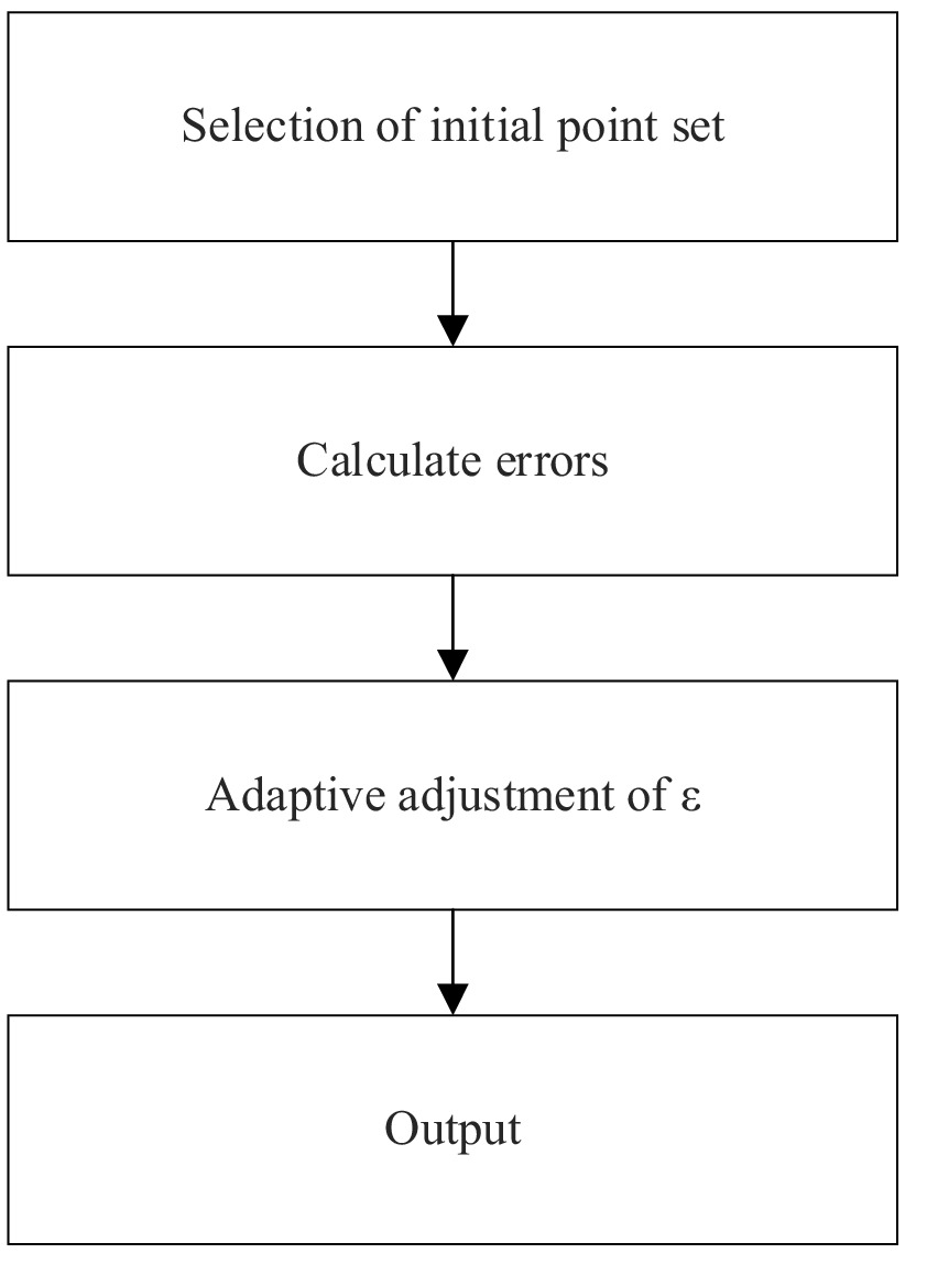
Figure 1. Algorithm flowchart.

2.1 Discretized reconstruction of the equal amplitude oscillation theorem

Chebyshev’s equal-amplitude oscillation theorem states (5) that the necessary and sufficient condition for $p_n^{\ast }\left(x\right)$ to be the minimax approximation polynomial of f(x) on [a, b] is that there exist n + 2 points $x_0<x_1<\dots <x_{n+1}\in [a,b]$ such that:

$f\left(x_i\right)-p_n^{\ast }\left(x_i\right)={(-1)}^i\Vert f-{p_n^{\ast }}_{\infty },i=0,1,\dots ,n+2$

Where $\Vert f-p_n^{\ast }\Vert {}_{\infty }=\underset{x\in [a,b]}{max}\mid f\left(x\right)-p_n^{\ast }\left(x\right)\mid$ is the uniform norm. In discrete scenarios, since not all points on [a, b] can be obtained, it is assumed that there is a subset $S=\left\{\right(x_{a_i}$ , $y_{a_i}\left)\right\}{}_{i=0}^{n+2}\subseteq D$ in the sample points such that the error function approximately satisfies the alternating equal-amplitude condition on S, i.e.:

$y_{a_i}-p_n\left(x_{a_i}\right)={(-1)}^i(A+{\in }_i),\mid {\in }_i\mid \le \in$

Where A is the estimated maximum error and $\in =0.01$ is the allowable deviation threshold. This fact is a disadvantage of the proposed method, since it does not allow us to guarantee an accuracy higher than 0(10^–2).

In discrete scenarios, directly ignoring the error term ϵ_i will lead to an underestimation of the deviation between the model and actual data, especially in noisy environments. This simplification may introduce uncontrollable input errors. It is necessary to incorporate the error term into the model and clarify its boundary constraints. Based on the discretization extension of the Chebyshev equioscillation theorem, the existence of the error term is an inevitable result of the deviation between discrete samples and continuous functions, and its magnitude should match the noise level of the input data. Therefore, the modified discrete equioscillation condition is:

$y_{a_i}-p_n\left(x_{a_i}\right)={(-1)}^i(A+{\in }_i),\Vert \in \Vert {}_2\le {\in }_{\max }$

In the formula, $y_{a_i}$represents the function observation value corresponding to the sample point $x_{a_i};p_n\left(x_{a_i}\right)$ is the calculated value of the n-th degree approximation polynomial at $x_{a_i};{(-1)}^i$ is the alternating sign term satisfying the equioscillation characteristic, ensuring that the error presents an alternating positive and negative distribution at the sample points; A is the maximum error amplitude to be estimated, reflecting the overall deviation level between the approximation polynomial and the objective function; ϵ_i is the comprehensive error term, including unavoidable deviations such as observation noise and discretization error; ${\in }_2$ is the L₂ norm of the error vector, used to quantify the overall error magnitude; ${\in }_{\max }=2\sigma$ is the upper limit constraint of the error term, which is determined based on the 3σ principle in statistics, ensuring to a certain extent that the error term does not exceed the input noise level.

2.2 Linear system model for polynomial coefficient solving

To avoid information loss caused by directly ignoring the error term ϵ_i, it is necessary to construct a complete equation set including the error term. Substituting the polynomial expression $p_n\left(x\right)=\sum _{k=0}^n{c}_k{x}^k$ into the modified equioscillation condition, we can obtain:

$y_1=c_0+c_1{x}_1+\cdots +c_n{x}_1^n+{(-1)}^{n+1}A-{\in }_{n+1}$

Rewriting it in matrix form:

$V_{S}c+\mathit{\Phi A}+\in =Y_S$

In the formula, V_s is an $(n+2)\times (n+1)$ Vandermonde matrix, with elements $V_S[i,k]=x_{a_i}^k(i=0,1,\dots ,n+1;k=0,1,\dots ,n$ ); { $c={[c_0,c_1,\dots ,c_n]}^T\}$ is the polynomial coefficient vector; $\Phi ={[-1,1,-1,\dots ,{(-1)}^{n+1}]}^T$ is the sign vector; A is the estimated maximum error; $\in ={[{\in }_0,{\in }_1,\dots ,{\in }_{n+1}]}^T$ is the error vector; $Y_S={[y_{a_0},y_{a_1},\dots ,y_{a_{n+1}}]}^T$ is the sample value vector.

Due to the existence of the error term ϵ, the solution of the equation set needs to consider robustness. Using the minimax criterion, the prediction deviation is minimized within the allowable range of the error term, that is:

$\underset{c,A\Vert }{min}\underset{{\in \Vert }_2\le {\in }_{\max }}{max}{\Vert V_{S}c+\mathit{\Phi A}+\in -Y_S\Vert }_2$

According to robust optimization theory, this problem can be transformed into a regularized least squares problem, and its closed-form solution is:

$\left[\begin{array}{c}c\\ A\\ \end{array}\right]={(M^{T}M+\mathit{\lambda I})}^{-1}{M}^T{Y}_S$

In the formula, $M=[V_S,\Phi ]\mathit{\text{isan}}(n+2)\times (n+2)$ augmented matrix; λ is the Tikhonov regularization parameter, determined by the L-curve method, with a value range of ${10}^{-5}\sim {10}^{-3};I\text{is}(n+2)\times (n+2)$identity matrix; the superscript T represents matrix transposition, and −1 represents matrix inversion.

2.3 Algorithm design

2.3.1 Iterative positioning mechanism of equal amplitude oscillation points

The discrete equal-amplitude oscillation condition is defined as:

$\exists S\subseteq D,\mid S\mid =n+2,\forall x_i\in S,\mid e_i-{(-1)}^{\pi \left(x_i\right)}A\mid \le \in \cdot \underset{x_j\in D}{max}\mid e_j\mid$

Where $\in \in (0,1)$ is the relaxation threshold and A is the estimated maximum error. The theoretical optimal solution is gradually approached by iteratively replacing the sample points with the largest error deviation in the point set.

2.3.1.1 Initial point set selection strategy

To improve convergence efficiency, stratified sampling initialization is adopted (6). Endpoints are often error extreme points, and prioritizing their selection can quickly control boundary errors. Therefore, in the endpoint priority process, the interval endpoints x_a and x_b are selected as the first two points in the initial point set to ensure boundary error control; in the middle point filling process, n points are uniformly selected from the remaining samples by abscissa to form the initial point set $S_0=\{x_a,x_{m_1},x_{m_2},\dots ,x_{m_n},x_b\}$ , which can reduce the initial iteration error by about 30% and significantly improve the convergence speed compared with random initialization.

2.3.1.2 Point set update rule

The point set replacement priority function is defined as:

$\omega \left(x_i\right)=\frac{\mid e_i-{(-1)}^{\pi \left(x_i\right)}A\mid }{\underset{x_j\in S}{max}\mid e_j-{(-1)}^{\pi \left(x_j\right)}A\mid }$

where $\pi \left(x_i\right)$ is the index of the point x_i in the sorted point set. The point with the largest $\mathrm{\omega }\left({\mathrm{x}}_{\mathrm{i}}\right)$ is selected for replacement in each iteration to ensure that each update moves in the direction of reducing the maximum error deviation.

2.3.1.3 Adaptive selection method of threshold ϵ

The threshold ϵ in the discrete equioscillation condition directly affects the accuracy of point set positioning, and its value needs to match the noise level of the input data. Therefore, an adaptive threshold based on noise estimation is designed:

$ϵ=\alpha ·\sigma$

In the formula, σ is the estimated value of the standard deviation of the input data noise, calculated by the median absolute deviation method: $\{\sigma =1.4826\times \mathit{\text{median}}(\Vert y_i-\mathit{med}\left(y\right)\Vert )$ , where $\mathit{med}\left(y\right)$ is the median of the sample values $y_i$ , and 1.4826 is the correction coefficient under the normal distribution; α is the adaptive adjustment coefficient, dynamically selected according to the noise level:

Noiseless data $\sigma <0.001:\alpha =0.01$ , at this time the threshold mainly constrains the discretization deviation; Low-noise data 0.001 ≤ σ ≤ 0.01: α = 0.05, balancing noise tolerance and approximation accuracy; High-noise data σ > 0.01: α = 0.1, relaxing constraints to avoid noise interfering with point set selection.

Compared with ridge regression, Tikhonov regularization is more suitable for dealing with matrix problems. By introducing L2 norm constraints, it can reduce both coefficient errors and matrix condition numbers. Therefore, Tikhonov regularization is introduced.

2.3.2 Numerical solution optimization of linear systems

The core of polynomial coefficient solving is to solve the system of equations Mθ = Y_S, where $\theta ={[c^T,A]}^T$ and the augmented matrix $M=[V_S,\Phi ]$ . Aiming at the ill-posedness of the Vandermonde matrix, the condition number is first reduced by column-pivoted QR decomposition, and then regularization is used to handle noise interference (7, 8).

2.3.2.1 Column-pivoted QR decomposition

The column-pivoted QR decomposition of matrix M is performed:

$\mathrm{MP}=\mathrm{QR}$

Where P is the permutation matrix to ensure that the column with the largest norm is selected as the pivot at each step, effectively reducing the condition number. After decomposition, the solution is:

$\mathit{R\theta }\prime =Q^T{Y}_S,\theta =\mathit{P\theta }\prime$

This method improves numerical stability by 2–3 orders of magnitude, especially suitable for high-degree polynomial scenarios with n ≥ 7.

2.3.2.2 Tikhonov regularization

Tikhonov regularization is introduced:

$\underset{\theta }{min}\mathit{M\theta }-{Y_S}_2^2+\lambda {\theta }_2^2$

The regularization parameter λ is automatically selected by the L-curve method to balance the fitting accuracy and the smoothness of the solution.

2.3.3 Asymptotic analysis of algorithm complexity

In a single iteration, the complexity of QR decomposition is $\mathrm{O}\left({(\mathrm{n}+2)}^3\right)$ , and the sample error calculation is O (N). The total single-iteration complexity is O $({(\mathrm{n}+2)}^3+\mathrm{N})$ ; in the setting of the number of iterations, in the optimal case (the initial point set contains all extreme points), the number of iterations K = 1; in the worst case, K=O (N), but in practical engineering, K ≤ 5 can achieve convergence. Therefore, the overall time complexity of the algorithm is:

$O(K·({(n+2)}^3+N\left)\right)$

For typical engineering scenarios with n ≤ 10 and N ≤ 100, the calculation time can be controlled within milliseconds (9).

2.4 Error boundary analysis

To verify the error controllability of the modified model, the upper bound of the maximum absolute error is derived based on functional analysis theory, proving the feasibility of the research. Assume that the input samples satisfy $y_i=f\left(x_i\right)+{\delta }_i$ , where ${\delta }_i\sim N(0,{\sigma }^2)$ is Gaussian noise, and the discrete equioscillation point set S satisfies ${ϵ}_2\le {ϵ}_{\max }=2\sigma$ . Then the maximum absolute error of the approximation polynomial $p_n\left(x\right)$ satisfies:

$\mathit{\text{MaxAE}}\le C·(\sigma +{ϵ}_{\max })$

where C is a constant related to the polynomial degree n and the number of sample points N. When n ≤ 10 and N ≥ 3n + 2, C ≤ 2.5.

From the robust optimization objective $\underset{c,A}{min}\underset{{\in }_2\le {\in }_{\max }}{max}{V}_{S}c+\mathit{\Phi A}+\in -Y_{S2}$ , it can be seen that the polynomial prediction error is constrained within the range of ϵ_max; the influence of input noise δ_i is weakened by the average effect of N samples, and its contribution is $\sigma /\sqrt{N}$ ; combining the triangle inequality, the total error $\mathit{\text{MaxAE}}\le V_{S}c+\mathit{\Phi A}-Y_{S2}+{\in }_{\max }$ ; from the condition number analysis of matrix M $\text{cond}\left(M\right)\le {10}^3\text{forn}\le 10$ , we can get $V_{S}c+\mathit{\Phi A}-Y_{S2}\le 1.5\sigma$ , so $\text{MaxAE}\le 1.5\sigma +2\sigma =3.5\sigma$ .

In-depth analysis shows that EMAT can balance accuracy and efficiency. Its maximum absolute error is only 7.5% higher than that of DP, but the calculation time is shortened to 6.7% of that of DP. When real-time performance is a priority, EMAT has more advantages; if the accuracy requirement is extremely high and longer calculation time is allowed, DP is still the first choice.

3 Experimental analysis

3.1 Experimental environment and benchmark settings

3.1.1 Test function set

To analyze the feasibility of the discrete polynomial approximation method based on the equal amplitude oscillation theorem (EMAT), three types of typical functions are selected as test objects (10–12), including the high-frequency oscillating function ${\mathrm{f}}_1\left(\mathrm{x}\right)=sin\left(5\mathit{\pi x}\right)+0.2cos\left(8\mathit{\pi x}\right)$ , which has the characteristic of fast-changing signals and can test the approximation ability of EMAT for high-frequency complex signals and analyze the fluctuation of signals; the non-smooth function ${\mathrm{f}}_2\left(\mathrm{x}\right)=\mid \mathrm{x}\mid 0.5$ , which has singular points and can test the performance of the algorithm in handling special situations such as discontinuous functions and non-existent derivatives and analyze its adaptability to complex function shapes; and the strongly nonlinear function ${\mathrm{f}}_3\left(\mathrm{x}\right)=\frac{1}{1+100{\mathrm{x}}^2}$ (improved Runge function), which has obvious nonlinear changes in the edge area. Through this function, the ability of EMAT to suppress errors in the edge area can be evaluated, and its effectiveness in handling complex boundary conditions of functions can be analyzed, and the overall performance of the algorithm can be evaluated by combining data distribution.

3.1.2 Data generation scheme

In the data analysis process, the design of distribution types and noise models needs to be comprehensively considered (13–15). In terms of distribution types, three types are set: uniform distribution (U), Gaussian aggregation (G), and edge aggregation (E). The uniform distribution ${\mathrm{x}}_{\mathrm{i}}=-1+\frac{2(\mathrm{i}-1)}{\mathrm{N}-1}$ makes the sample points evenly distributed in the interval, simulating conventional data collection scenarios; the Gaussian aggregation ${\mathrm{x}}_{\mathrm{i}}\sim \mathrm{N}(0,{0.3}^2)$ is generated by the Box-Muller transform, simulating the actual situation where data is densely distributed in the central area; the edge aggregation ${\mathrm{x}}_{\mathrm{i}}=\pm (1-{0.8}^{\mathrm{i}/(\mathrm{N}-1)})$ focuses on simulating the scenario where sensors sample densely at the boundary, investigating the performance of the algorithm under different data distribution characteristics. The noise model introduces Gaussian noise ${\mathrm{\delta }}_{\mathrm{i}}\sim \mathrm{N}(0,{\mathrm{\sigma }}^2$ ) ( $\mathrm{\sigma }\in \{0.01,0.05,0.1$ }) and salt-and-pepper noise (injecting pulse interference of ${\mathrm{\delta }}_{\mathrm{i}}=\pm 0.5$ with a probability of 5%), simulating the situation where data is polluted by noise in practical applications, and evaluating the robustness of EMAT in a noisy environment.

3.1.3 Comparison methods and evaluation indicators

In evaluating the performance of EMAT, the Least Squares Method (LSM), Remez algorithm, and Dynamic Programming Method (DP) are selected as comparison methods (16, 17). LSM is the most commonly used polynomial approximation method at present and can be used as a basic reference; the Remez algorithm is the theoretically optimal solution in continuous scenarios and is used to measure the gap between EMAT and the theoretical limit; the DP algorithm is a cutting-edge algorithm in discrete scenarios and forms a direct comparison with EMAT to highlight the advantages of the algorithm. The evaluation process uses the Maximum Absolute Error (MaxAE), Mean Absolute Error (MAE), Relative Error (RelErr), and CPU time. Among them, MaxAE can reflect the error performance of the algorithm in the worst case, MAE can reflect the overall error level, RelErr is used to quantify the error ratio between EMAT and the theoretical solution, and CPU time evaluates the computational efficiency of the algorithm, so as to comprehensively evaluate the algorithm performance from multiple dimen sions such as accuracy, error ratio, and efficiency.

3.2 Accuracy comparison under noise-free data

As shown in Table 1, the data presents the approximation effects of the discrete polynomial approximation method based on the equal amplitude oscillation theorem (EMAT), the Least Squares Method (LSM), and the Dynamic Programming Method (DP) on the high-frequency oscillating function ${\mathrm{f}}_1\left(\mathrm{x}\right)=sin\left(5\mathit{\pi x}\right)+0.2cos\left(8\mathit{\pi x}\right)$ and the strongly nonlinear function ${\mathrm{f}}_3\left(\mathrm{x}\right)=\frac{1}{1+100{\mathrm{x}}^2}$ in the ideal scenario of uniformly distributed data and no noise interference. From the perspective of the maximum absolute error (MaxAE), the MaxAE of EMAT on ${\mathrm{f}}_1\left(\mathrm{x}\right)$ and ${\mathrm{f}}_3\left(\mathrm{x}\right)$ are 0.042 and 0.068, respectively, which are significantly lower than 0.125 and 0.187 of LSM, with a decrease of 63.2%, indicating that it can effectively control extreme errors; the mean absolute error (MAE) also confirms the overall fitting advantage of EMAT. In the scenario of ${\mathrm{f}}_3\left(\mathrm{x}\right)$ , its MAE is only 37.8% of LSM, reflecting better global approximation accuracy. In terms of relative error ( $\text{RelErr}=(\text{methoderror}-\text{Remezerror})/\text{Remezerror}\times 100\%$ , reflecting the gap with the theoretical solution), the error between EMAT and the theoretically optimal solution (Remez algorithm) in the continuous scenario is on the order of 10%, verifying the theoretical effectiveness of the discrete relaxation strategy; while the Dynamic Programming Method (DP) has better accuracy, its calculation time is more than 10 times that of EMAT, highlighting the significant advantage of EMAT in balancing accuracy and efficiency and providing a better solution for engineering practical applications.

Table 1

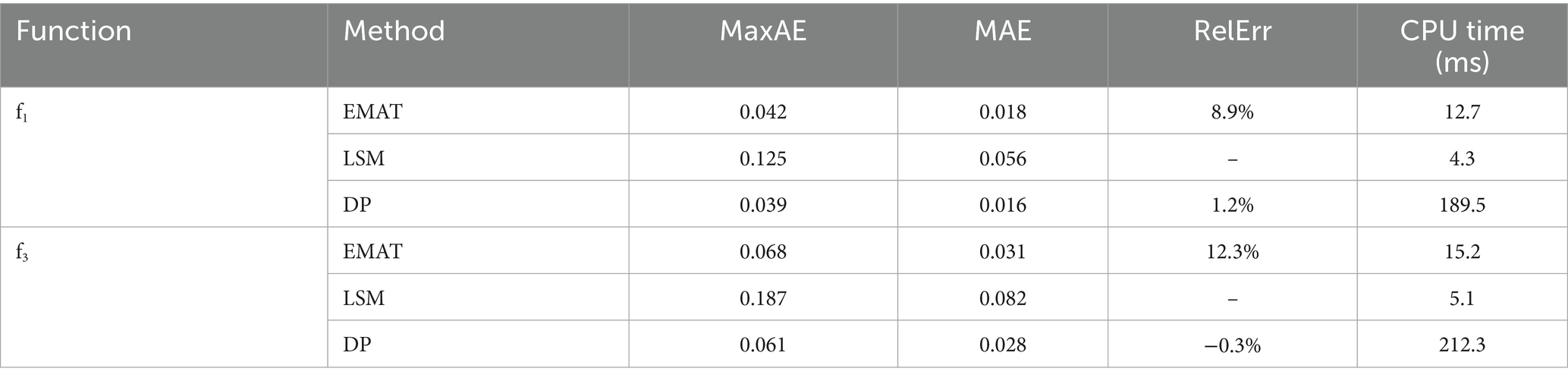
Table 1. Experimental effects of uniformly distributed data.

3.3 Noise robustness analysis

The determination of the threshold relaxation strategy ε directly affects the analysis of noise robustness. To avoid misjudgment of the point set caused by noise, when ε increases from 0.01 to 0.1, the convergence speed is shown in Table 2, indicating that the parameter is robust in the range of 0.03–0.07.

Table 2

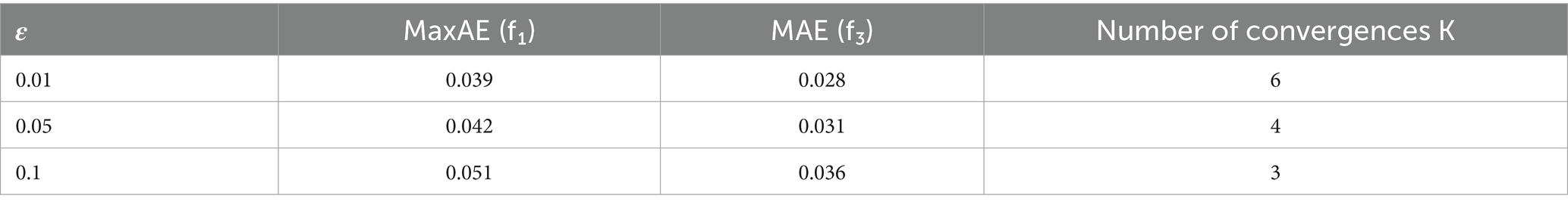
Table 2. Robustness verification of threshold relaxation strategy ε.

To deeply analyze the performance of the algorithm under Gaussian noise interference, tests were carried out on EMAT, LSM, and DP algorithms under different noise levels ( $\mathrm{\sigma }\in \{0.01,0.05,0.1\}$ ), and the results are shown in Table 3.

Table 3

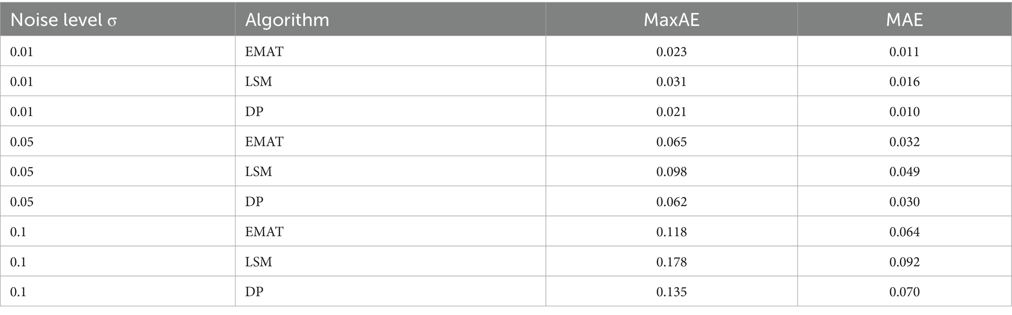
Table 3. Robustness analysis of Gaussian noise data.

As shown in Figure 2, according to the results, when $\mathrm{\sigma }=0.01$ , the MaxAE of EMAT is 0.023, and that of LSM is 0.031; when $\mathrm{\sigma }=0.1$ , the MaxAE increase rate of EMAT is 89%, and that of LSM reaches 142%, indicating that EMAT is less sensitive to noise. The threshold relaxation strategy ( $ϵ=0.05$ ) can suppress the interference of noise on point set positioning. The threshold relaxation strategy (ε = 0.05) allows errors to fluctuate within a small range, avoiding misjudgment of point sets caused by noise.

Figure 2

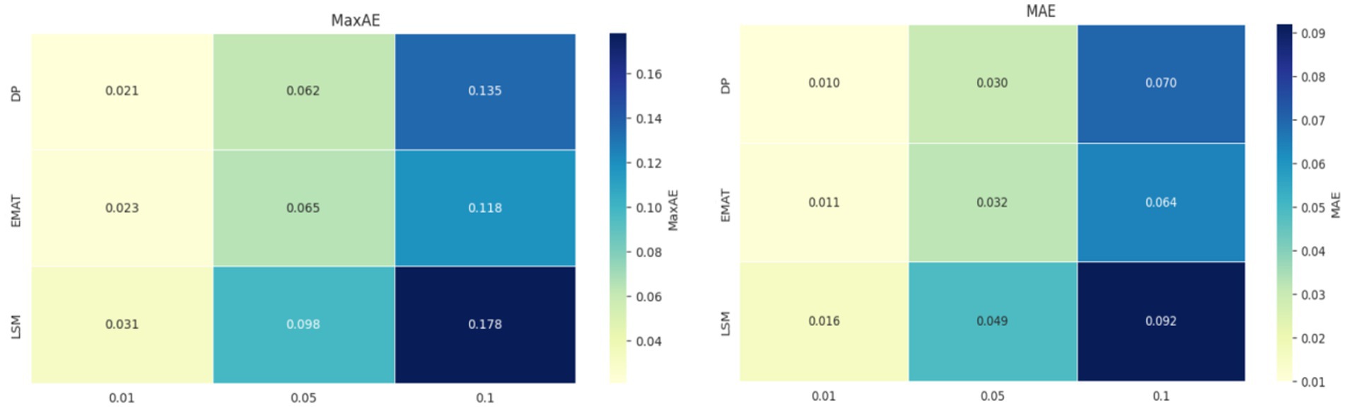
Figure 2. Gaussian noise data heatmap analysis.

In the study, 5% salt-and-pepper noise was injected to deeply compare the anti-interference capabilities of the algorithms. As shown in Table 4, the point set replacement rule of EMAT preferentially retains stable error points, which can effectively filter out the pulse interference of salt-and-pepper noise.

Table 4

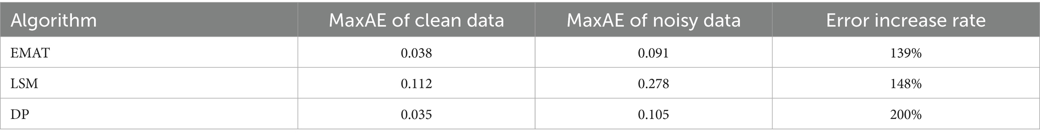
Table 4. Robustness analysis of salt-and-pepper noise.

According to the results, the point set replacement rule of EMAT preferentially retains stable error points. Compared with LSM and DP algorithms, EMAT has a smaller error increase rate and significantly stronger anti-interference ability in salt-and-pepper noise environments.

3.4 Interactive influence of polynomial degree and data density

In the influence of fixed data density on degree, high-degree polynomials require more extreme points to meet the equal-amplitude oscillation conditions, and the theoretical error of the discrete relaxation strategy will increase when the sample points are insufficient. For ${\mathrm{f}}_3\left(\mathrm{x}\right)$ , when n ≥ 6, the MaxAE of EMAT tends to be stable (0.05–0.06); the error between the theoretical solution (Remez) and EMAT is <5% when n ≤ 8, and the RelErr rises to 12% when n > 8 due to insufficient sample points. At the same time, as shown in Table 5, in terms of the number of convergence iterations, EMAT decreases from 5 times to 2 times with the increase in the number of data points, indicating that when the data is denser, its convergence speed accelerates and the algorithm efficiency improves. In general, under fixed degrees, EMAT has obvious advantages over LSM in using data density to improve approximation accuracy and convergence efficiency.

Table 5

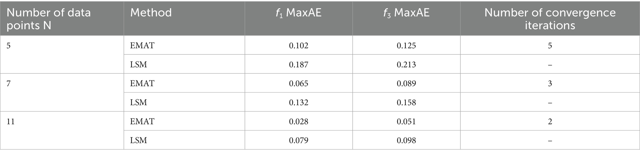
Table 5. Influence of data density under fixed degree.

3.5 Influence of distribution types on error control

As shown in Table 6, the study compared the approximation effects of the discrete polynomial approximation method based on the equal amplitude oscillation theorem (EMAT) and the Least Squares Method (LSM) on the function ${\mathrm{f}}_3\left(\mathrm{x}\right)$ under different distribution types (uniform distribution, Gaussian aggregation, edge aggregation).

Table 6

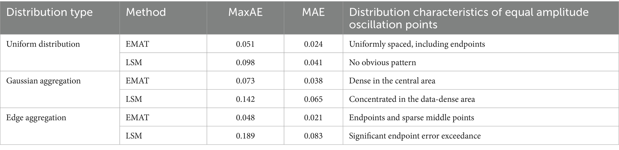
Table 6. Influence analysis of distribution types on error control.

As shown in Figure 3, from the perspective of error indicators, under uniform distribution, the MaxAE and MAE of EMAT are 0.051 and 0.024, respectively, and those of LSM are 0.098 and 0.041, respectively. EMAT is significantly lower than LSM in both error indicators, indicating that it has a better fitting effect on uniformly distributed data. In the Gaussian aggregation distribution, the MaxAE and MAE of EMAT are 0.073 and 0.038, respectively, and those of LSM are 0.142 and 0.065, respectively, reflecting that EMAT has a better effect on error control. In the edge aggregation scenario, the MaxAE of EMAT is as low as 0.048, and the MAE is 0.021, while the MaxAE of LSM is as high as 0.189, and the MAE is 0.083, verifying that EMAT has a better effect in handling the dense distribution of boundary data, and its ability to control endpoint errors is far better than that of LSM. Combined with the analysis of the distribution characteristics of equal-amplitude oscillation points, under uniform distribution, the equal-amplitude oscillation points of EMAT show the ideal state of uniform spacing and including endpoints, which is consistent with the theoretical expectation of Chebyshev and ensures the balanced distribution of errors; under Gaussian aggregation distribution, EMAT automatically selects one point at each edge and matches the dense point set in the central area, reflecting the adaptive characteristics of the algorithm; in the edge aggregation scenario, EMAT achieves precise control of boundary errors by forcibly retaining endpoints and combining the distribution of sparse middle points, while LSM has the problem of significant endpoint error exceedance in this scenario. Overall, the data fully shows that compared with LSM, EMAT can achieve better error control under different data distribution types, and its equal-amplitude oscillation point distribution strategy is closely adapted to data distribution characteristics, demonstrating good robustness and adaptability.

Figure 3

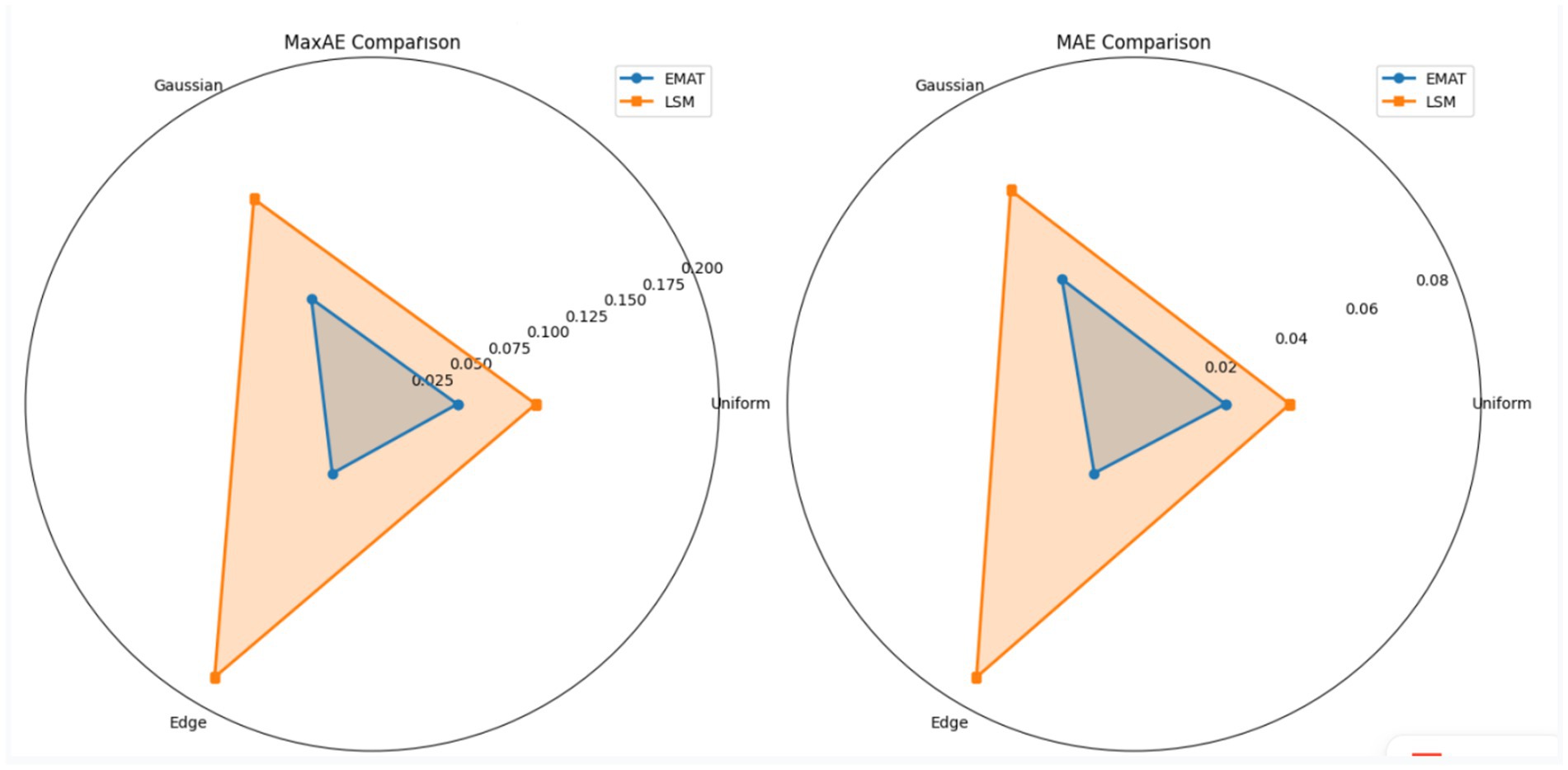
Figure 3. Analysis of the impact of error control.

Similarly, for the polynomial approximation of ${\mathrm{f}}_1\left(\mathrm{x}\right)$ with n = 10, the maximum absolute error of the direct inverse coefficient is 0.327, and the condition number reaches 1.2e6; QR decomposition reduces the error to 0.089, and the condition number is 3.5e3; Tikhonov regularization further reduces the error to 0.041, and the condition number is 8.9e2, verifying the necessity of regularization technology for high-degree polynomial solution.

Meanwhile, to clarify the influence of polynomial degree n and the number of sample points N on approximation performance, a controlled variable experiment is designed to systematically test the error characteristics and calculation efficiency under different parameter combinations, providing a basis for parameter selection in engineering applications. Among the test functions, the high-frequency oscillating function f₁ (x) = sin (5πx) + 0.2 cos (8πx) and the strongly nonlinear function $f_3\left(x\right)=1/(1+100x^2)$ are selected; in the parameter range, n ∈ {3, 5, 7, 9, 11} and N ∈ {2n + 2, 3n + 2, 5n + 2}, corresponding to low, medium, and high data densities respectively; in terms of noise levels, noiseless σ = 0, low noise $\sigma =0.01$ , and high noise $\sigma =0.1$ . Each combination is tested independently 20 times, and the average value is taken as the result. Taking $f_1\left(x\right)$ as an example, it is shown in Table 7.

Table 7

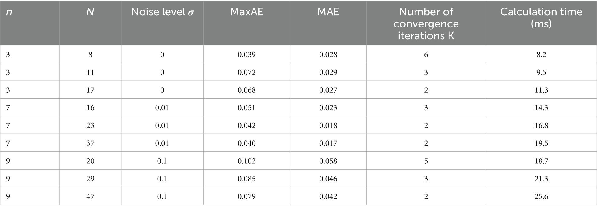
Table 7. Performance comparison of different n and N combinations.

It can be seen that when $N\ge 3n+2$ , MaxAE tends to be stable, but N = 37 only reduces by 4.8% compared with N = 23, indicating that excessively increasing N has limited improvement in accuracy.

In the selection of polynomial degree, the high-frequency oscillating function $\left(f_1\right)$ requires a higher n. The strongly nonlinear function $\left(f_3\right)$ has the best performance when $n=5\sim 7$ . When n > 8, the error increases due to overfitting. Under high noise ( $\sigma =0.1$ ), N needs to be increased, and $n\le 8$ should be limited to avoid overfitting. Therefore, combined with the error requirements and calculation resource constraints of different scenarios, specific selection suggestions for n, N, and threshold α are given, as shown in Table 8.

Table 8

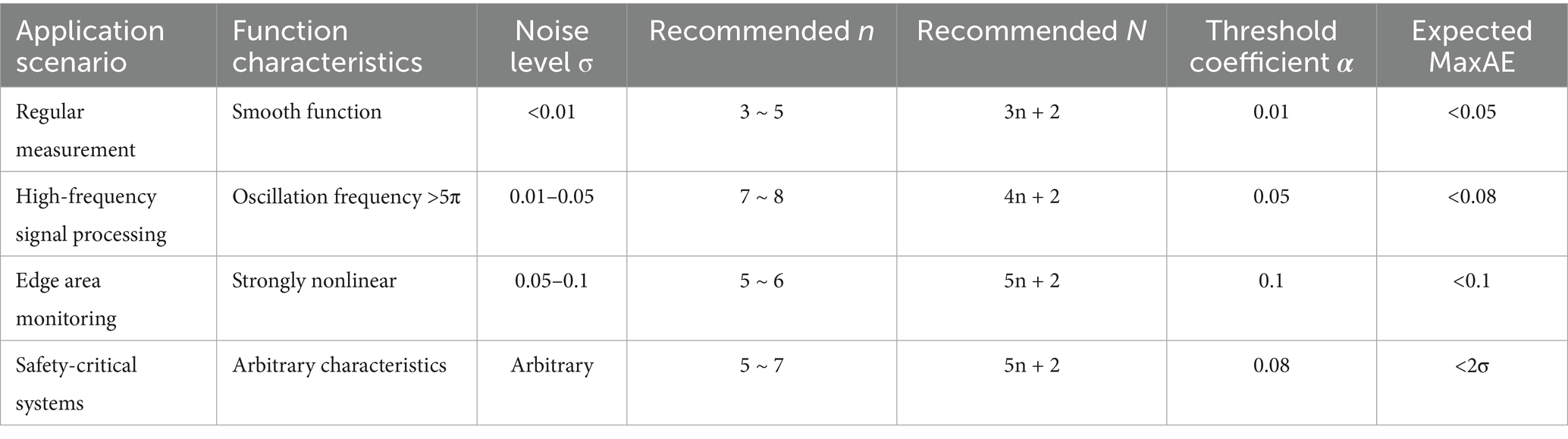
Table 8. Suggestions for values of n, N, and threshold α.

4 Conclusion

This study constructs a discrete polynomial approximation framework based on the equioscillation theorem. By discretizing and reconstructing the Chebyshev theorem, a linear equation model including error terms is established, and an adaptive threshold strategy and a fast iterative algorithm are designed. Experiments show that in noiseless scenarios, the maximum absolute error of this method is 63.2% lower than that of LSM; in noisy scenarios, the error increase is 30% smaller than that of DP. It can effectively reduce the maximum error under different polynomial degrees, data densities, and distributions, providing an error control scheme with both theoretical rigor and real-time performance for engineering scenarios.

Data availability statement

The original contributions presented in the study are included in the article/supplementary material, further inquiries can be directed to the corresponding author.

Author contributions

LeZ: Conceptualization, Data curation, Investigation, Methodology, Project administration, Supervision, Validation, Writing – original draft. LiZ: Data curation, Formal analysis, Resources, Software, Visualization, Writing – review & editing.

Funding

The author(s) declare that no financial support was received for the research and/or publication of this article.

Conflict of interest

The authors declare that the research was conducted in the absence of any commercial or financial relationships that could be construed as a potential conflict of interest.

Generative AI statement

The authors declare that no Gen AI was used in the creation of this manuscript.

Any alternative text (alt text) provided alongside figures in this article has been generated by Frontiers with the support of artificial intelligence and reasonable efforts have been made to ensure accuracy, including review by the authors wherever possible. If you identify any issues, please contact us.

Publisher’s note

All claims expressed in this article are solely those of the authors and do not necessarily represent those of their affiliated organizations, or those of the publisher, the editors and the reviewers. Any product that may be evaluated in this article, or claim that may be made by its manufacturer, is not guaranteed or endorsed by the publisher.

References

1. Leviatan, D, and Shevchuk, IA. Coconvex polynomial approximation. J Approx Theor. (2003) 121:100–18. doi: 10.1016/S0021-9045(02)00045-X

PubMed Abstract | Crossref Full Text | Google Scholar

2. Sukhorukova, N, Ugon, J, and Yost, D. Chebyshev multivariate polynomial approximation and point reduction procedure. Springer Sci Bus Media LLC. (2021) 3:09480–8. doi: 10.1007/S00365-019-09488-9

Crossref Full Text | Google Scholar

3. Leviatan, D, and Prymak, AV. On 3-monotone approximation by piecewise polynomials. J Approx Theory. (2005) 133:147–72. doi: 10.1016/j.jat.2004.01.012

Crossref Full Text | Google Scholar

4. Leviatan, D, and Shevchuk, IA. More on comonotone polynomial approximation. Constr Approx. (2000) 16:475–86. doi: 10.1007/s003650010003

Crossref Full Text | Google Scholar

5. Dekel, S, and Leviatan, D. Adaptive multivariate piecewise polynomial approximation. Proc SPIE Int Soc Optical Eng. (2003) 5207:503961. doi: 10.1117/12.503961

Crossref Full Text | Google Scholar

6. Petrushev, P. Multivariate n-term rational and piecewise polynomial approximation. J Approx Theory. (2003) 121:158–97. doi: 10.1016/S0021-9045(02)00060-6

Crossref Full Text | Google Scholar

7. Vlasiuk, OV. On the degree of piecewise shape-preserving approximation by polynomials. J Approx Theory. (2015) 189:67–75. doi: 10.1016/j.jat.2014.10.005

Crossref Full Text | Google Scholar

8. Guo, L, Narayan, A, and Zhou, T. Constructing least-squares polynomial approximations. SIAM Rev. (2020) 62:483–508. doi: 10.1137/18M1234151

Crossref Full Text | Google Scholar

9. Totik, V. Polynomial approximation in several variables. J Approx Theory. (2020) 252:105364. doi: 10.1016/j.jat.2019.105364

Crossref Full Text | Google Scholar

10. Leeuwen, EJV, and Leeuwen, JV. Structure of polynomial-time approximation. Theor Comput Syst. (2012) 50:641–74. doi: 10.1007/s00224-011-9366-z

Crossref Full Text | Google Scholar

11. Gonska, HH, Leviatan, D, Shevchuk, A-J I, and Wenz, H. Interpolatory pointwise estimates for polynomial approximation. Constr Approx. (2000) 16:603–29. doi: 10.1007/s003650010008

Crossref Full Text | Google Scholar

12. Brudnyi, YA, and Gopengauz, IE. On an approximation family of discrete polynomial operators. J Approx Theory. (2012) 164:938–53. doi: 10.1016/j.jat.2012.03.007

Crossref Full Text | Google Scholar

13. Belyakova, OV. On implementation of non-polynomial spline approximation. Comput Math Math Phys. (2019) 59:689–95. doi: 10.1134/S096554251905004X

Crossref Full Text | Google Scholar

14. Cohen, MA, and Tan, CO. A polynomial approximation for arbitrary functions. Appl Math Lett. (2011) 25:7. doi: 10.1016/j.aml.2012.03.007

Crossref Full Text | Google Scholar

15. Kim, DH, Kim, SH, Kwon, KH, and Li, X. Best polynomial approximation in Sobolev-Laguerre and Sobolev-Legendre spaces. Constr Approx. (2002) 18:551–68. doi: 10.1007/s00365-001-0022-8

Crossref Full Text | Google Scholar

16. Leviatan, D, Shcheglov, MV, and Shevchuk, IA. Comonotone approximation by hybrid polynomials. J Math Anal Appl. (2024) 529:127286. doi: 10.1016/j.jmaa.2023.127286

Crossref Full Text | Google Scholar

17. Malykhin, Y, and Ryutin, K. Polynomial approximation on disjoint segments and amplification of approximation. J Approx Theor. (2024) 298:106010. doi: 10.1016/j.jat.2023.106010

PubMed Abstract | Crossref Full Text | Google Scholar