Epidemic dynamics in the spatio-temporal predator-prey model

In this work, we develop a novel mathematical model to simulate the spatio-temporal dynamics of epidemics in a predator–prey system. The model integrates the classical Lotka–Volterra predator–prey framework with a Susceptible–Infected–Susceptible disease model and explicitly incorporates diffusion terms to capture spatial movement. This unified approach allows us to simultaneously analyze susceptible and infected prey and predator populations, and account for both ecological and spatial interactions. An extension beyond traditional models that often treat these processes separately. The model consists of four partial differential equations and includes key ecological factors such as growth and mortality rates, predation, reproduction, and carrying capacity. Through extensive numerical simulations across a wide range of ecological and epidemiological parameters, we systematically investigate how disease transmission and spatial diffusion shape population dynamics. The results reveal that spatial movement plays a critical role in determining species distribution and infection persistence, highlighting the complex interplay between disease spread and ecosystem stability.

1 Introduction

In mathematical biology, understanding interactions among species and the transmission of infectious diseases is essential to predict outbreaks, formulate effective control strategies, and support ecosystem management initiatives as discussed by Montevil [1]. Two foundational models in this field are the Lotka–Volterra (LV) predator-prey model studied by Swailem and Täuber [2], and the Susceptible–Infected–Susceptible (SIS) epidemiological model, described by Kuhl [3]. The Lotka–Volterra model describes predator–prey dynamics through a system of nonlinear differential equations and has been widely employed to capture the cyclical dynamics of such relationships, where the population sizes of both species oscillate over time. In contrast, the SIS model partitions a host population into susceptible and infective compartments and describes the rates at which individuals transition between these states. This model is particularly useful for describing diseases with temporary immunity and informs the development of effective control strategies.

The classical LV framework has been extended to include additional ecological complexities, such as inter-species competition, mutualism, and environmental stochasticity. For example, recent studies by Shaikhet and Korobeinikov [4] have investigated the asymptotic behavior of LV models under stochastic disturbances to demonstrate the influence of random fluctuations on population stability and persistence. In addition, Davis et al. [5] adapted the model to quantify interactions within microbial communities to show its versatility in the analysis of a wide range of biological systems. Similarly, the SIS model has evolved significantly to incorporate spatial heterogeneity, behavioral responses, and stochastic effects to reflect realistic epidemiological dynamics. For stochastic SIS models, Lahrouz et al. [6] and Gray et al. [7] have explored the influence of random perturbations on extinction or persistence of the disease to reveal critical thresholds for long-term endemicity. Similarly, Pastor-Satorras et al. [8] applied network-based SIS frameworks to study the transmission of disease in complex social and contact networks to inform the design of targeted interventions and control strategies.

To better understand the interactions between ecological dynamics and disease transmission, many studies have integrated classical LV dynamics with SIS-type infection models. These hybrid frameworks reveal how disease can influence species interactions, population stability, and long-term infection persistence in ecological systems [9]. An early influential contribution by Hadeler and Freedman [10] introduced a predator–prey model and incorporated SI-type infection into the prey population. The study demonstrated how the dynamics of the disease could fundamentally affect the survival of predator and alter the overall stability of the ecosystem. Since then, this modeling approach has been extended in various ecological contexts to examine how the dynamics of a disease shapes the coexistence and long-term behavior of a system (see, e.g., [9, 11–13]). Complementing these advances, Gómez-Hernández et al. [14] provided a comprehensive review of ODE-based eco-epidemic predator–prey models. Their work systematically classified recent model structures and identified key gaps, particularly the limited incorporation of infection dynamics, spatial heterogeneity, and delay effects. This gap is beginning to narrow; for instance, Majee et al. [15] recently introduced a spatiotemporal eco-epidemic model which incorporates both incubation and gestation delays.

Eco-epidemiological models play a crucial role in understanding temporal dynamics. However, many classical models assume spatial homogeneity and therefore overlook localized interactions among individuals or species. Motivated by this limitation, researchers such as Davydovych et al. [16] and Naz and Torrisi [17] have incorporated diffusion terms into ecological and epidemiological models to capture the spatial spread of populations and diseases. These spatially explicit models have revealed important spatiotemporal phenomena. For example, Hu et al. [18] demonstrated the emergence of spatial pattern formation in predator–prey systems, while Zhao and Ruan [19] identified traveling wavefronts as key mechanisms for disease propagation. Further, Chen and Wu [20] highlighted the role of spatial thresholds in determining the persistence or extinction of a disease. The study of reaction–diffusion eco-epidemiological systems continues to advance through a combination of analytical and numerical approaches. Contributions by Hu et al. [18], Qiao et al. [21], Ling et al. [22], Sun et al. [23], and Upadhyay and Roy [24] have contributed to the expanding literature showing how traveling waves, pattern formation, bifurcation structures, and instabilities can emerge and govern the behavior of the system.

Recent work has extended classical reaction-diffusion frameworks to investigate the influence of prey-taxis on solution behavior in eco-epidemiological models. In particular, Upadhyay et al. [25] employed the p-Laplacian to model slow dispersal and incorporated increased mortality among infected prey. The authors proved the global existence of classical solutions under standard mortality and random movement and established weak solutions under conditions of slow dispersal and elevated mortality. Assuming linear diffusion and predator taxis toward infected prey, they analyzed the stability of the positive equilibrium and demonstrated the emergence of steady-state bifurcations. These complex dynamics were further illustrated through numerical simulations, underscoring important implications for biological invasions and pest control in disease-affected populations. In a related work, Peng et al. [26] studied a reaction-diffusion SIS epidemic model that featured a non-linear incidence term of the form S^qI^p (0 < p ≤ 1, q>0) and a constant total population. They analyzed the spatial profiles of endemic equilibria under conditions of limited movement for both susceptible and infected individuals and revealed how non-linear transmission mechanisms and reduced mobility jointly shape the spread of disease. Their theoretical results, supported by numerical simulations, highlighted the role of spatial heterogeneity and complex transmission on epidemic dynamics.

Previous studies and reviews have emphasized the importance of spatial thresholds and wave phenomena in shaping the dynamics of outbreak, particularly in eco-epidemiological systems (e.g., [16, 17]). From a computational perspective, Biswas and Bairagi [27] demonstrated that nonstandard finite difference methods preserve critical biological properties more effectively than traditional Euler schemes, while Liu and Yang [28] used implicit–explicit methods to improve the computational efficiency and stability in reaction-diffusion SIS models. Furthermore, Sorokin and Vyazmin [29] emphasized the importance of tailored numerical schemes in delayed systems, especially to capture time-lagged spatial effects and heterogeneity.

Although many eco-epidemiological models have been proposed, most assume only one infected species or neglect the role of spatial structure, which is essential in shaping ecosystem behavior [15]. Comprehensive frameworks that simultaneously capture infection in both predator and prey populations, while incorporating spatial dynamics, remain relatively scarce. To address this gap, we develop a spatially explicit model that captures the joint dynamics of disease and predator–prey interactions. Our framework includes susceptible and infected compartments for both predators and prey, and incorporates diffusion to model local movement. The resulting system of four coupled partial differential equations accounts for predation, recovery, transmission, and logistic growth. Using numerical simulations, we analyze how spatial and ecological parameters influence long-term outcomes, revealing conditions for disease persistence, species coexistence, and ecosystem stability. These results provide realistic insights relevant to conservation planning and infectious disease management.

The remainder of the paper is organized as follows. In Section 2, we introduce the mathematical model that includes four compartments: susceptible and infected individuals in predator and prey populations. Section 3 presents the spatial extension of the model by incorporating diffusion terms, along with its numerical approximation using the explicit Euler method in time and a cell-centered finite-difference scheme in space. Section 4 provides numerical results for three cases: (1) the impact of varying predator-prey parameters, (2) effects of varying epidemic parameters, and (3) effect of varying diffusion. The paper concludes with a summary of key findings and suggestions for future research directions.

2 Mathematical model

We propose a combined model that integrates the dynamics of disease into the predator-prey framework by incorporating both susceptible and infected classes for predator and prey populations. Details about predator-prey model and disease spread can be found in the Appendix A. The model is designed to investigate how infection alters interspecies interactions and influences the stability and long-term behavior of population sizes. By capturing these dynamics, the approach allows for a detailed examination of population trends and facilitates the assessment of disease impact and other ecological factors on the overall ecosystem. Based on the established ecological and epidemiological modeling frameworks by Krebs [30], Murray [31], Rojas and Mena-Lorca [32], Gog and Swinton [33], Santos and Morais [34], Bjørnstad and Grenfell [35], and He and Li [36], the following assumptions are used to develop the model.

1. The prey population finds abundant food all the time.

2. The prey population is self-limiting and exhibits logistic growth in the absence of predator. The size of the prey population influences the growth of the predator population, while natural mortality is incorporated for both species.

3. The disease is transmitted between predator and prey populations.

4. Infected individuals recover and subsequently re-enter the susceptible class.

5. Infected prey reproduce only susceptible offspring.

6. The food supply of the predator population depends on the prey population.

Based on the stated assumptions, the epidemic dynamics within the predator-prey system are modeled by integrating the SIS framework, as defined in Equation 21, with the classical Lotka-Volterra predator-prey equations presented in Equation 23.

Let u_s be a susceptible prey population, u_i be an infected prey population, v_s be a susceptible predator population and v_i be an infected predator population. The evolution of these populations is described by the following system of differential equations

$\begin{array}{l}\frac{\partial u_s}{\partial t}={\alpha }_s{u}_s+{\alpha }_i{u}_i-{\beta }_s^s{u}_s{v}_s-{\beta }_i^s{u}_s{v}_i-{\gamma }_s^u{u}_s^2-{\sigma }_i^s{u}_s{u}_i\\ -{\sigma }_{vi}^s{u}_s{v}_i+{\omega }_i{u}_i,\\ \frac{\partial u_i}{\partial t}=-{\beta }_s^i{u}_i{v}_s-{\beta }_i^i{u}_i{v}_i-{\gamma }_i^u{u}_i^2+{\sigma }_i^s{u}_s{u}_i+{\sigma }_{vi}^s{u}_s{v}_i-{\omega }_i{u}_i,\\ \frac{\partial v_s}{\partial t}=-{\gamma }_s^v{v}_s+{\delta }_s^s{v}_s{u}_s+{\delta }_i^s{v}_s{u}_i-{\sigma }_i^{vs}{v}_s{u}_i-{\sigma }_{vi}^{vs}{v}_s{v}_i+{\omega }_{vi}{v}_i,\\ \frac{\partial v_i}{\partial t}=-{\gamma }_i^v{v}_i+{\delta }_s^i{v}_i{u}_s+{\delta }_i^i{v}_i{u}_i+{\sigma }_i^{vs}{v}_s{u}_i+{\sigma }_{vi}^{vs}{v}_s{v}_i-{\omega }_{vi}{v}_i,& (1)\end{array}$

where α_s is the intrinsic growth rate of susceptible prey, α_i is the intrinsic growth rate of infected prey, ${\beta }_s^s$ is the predation rate of susceptible predators on susceptible prey, ${\beta }_i^s$ is the predation rate of infected predators on susceptible prey, ${\beta }_s^i$ is the predation rate of susceptible predators on infected prey, ${\beta }_i^i$ is the predation rate of infected predators on infected prey, ${\gamma }_s^u$ is the density-dependent mortality rate of susceptible prey, ${\gamma }_i^u$ is the density-dependent mortality rate of infected prey, ${\gamma }_s^v$ is the intrinsic mortality rate of susceptible predators, ${\gamma }_i^v$ is the intrinsic mortality rate of infected predators, ${\delta }_s^s$ is the reproduction rate of susceptible predators from consuming susceptible prey, ${\delta }_i^s$ is the reproduction rate of susceptible predators from consuming infected prey, ${\delta }_s^i$ is the reproduction rate of infected predators from consuming susceptible prey, ${\delta }_i^i$ is the reproduction rate of infected predators from consuming infected prey, ${\sigma }_i^s$ is the rate of disease transmission from infected prey to susceptible prey, ${\sigma }_{vi}^s$ is the rate of disease transmission from infected predators to susceptible prey, ${\sigma }_i^{vs}$ is the rate of disease transmission from infected prey to susceptible predators, ${\sigma }_{vi}^{vs}$ is the rate of disease transmission from infected predators to susceptible predators, ω_i is the rate at which infected prey recover and become susceptible, ω_vi is the rate at which infected predators recover and return to the susceptible state.

The system (Equation 1) is supplemented with the following initial conditions:

$u_s(0)=u_s^0,u_i(0)=u_i^0,v_s(0)=v_s^0,v_i(0)=v_i^0,t=0.$

To better understand a complex interaction presented in Equation 1, we consider two special cases of the model: one without predator-prey interaction, and another that neglects epidemic transmission.

2.1 Susceptible-infected-susceptible model for two species without species interaction

In this special case of the general model (Equation 1), we focus solely on the processes of infection transmission and recovery. Susceptible prey become infected by contact infected prey or infected predators. After a certain period, the infected prey can recover and return to the susceptible class. Consequently, the equations for the susceptible prey population (u_s(t)) and the infected prey population (u_i(t)) are given as follows

$\begin{array}{ll}\begin{array}{c}\frac{\partial u_s}{\partial t}=-{\sigma }_i^s{u}_s{u}_i-{\sigma }_{vi}^s{u}_s{v}_i+{\omega }_i{u}_i,\\ \frac{\partial u_i}{\partial t}={\sigma }_i^s{u}_s{u}_i+{\sigma }_{vi}^s{u}_s{v}_i-{\omega }_i{u}_i,\end{array}& (2)\end{array}$

where ${\sigma }_i^s$ is the transmission rate of infection from infected prey to susceptible prey, ${\sigma }_{vi}^s$ is the transmission rate of infection from infected predators to susceptible prey, and ω_i is the recovery rate of infected prey to susceptible prey.

The susceptible predator population (v_s(t)) and the infected predator population (v_i(t)) are given as follows

$\begin{array}{ll}\begin{array}{c}\frac{\partial v_s}{\partial t}=-{\sigma }_i^{vs}{v}_s{u}_i-{\sigma }_{vi}^{vs}{v}_s{v}_i+{\omega }_{vi}{v}_i,\\ \frac{\partial v_i}{\partial t}={\sigma }_i^{vs}{v}_s{u}_i+{\sigma }_{vi}^{vs}{v}_s{v}_i-{\omega }_{vi}{v}_i,\end{array}& (3)\end{array}$

where ${\sigma }_i^{vs}$ is the transmission rate of infection from infected prey to susceptible predator, ${\sigma }_{vi}^{vs}$ is the transmission rate of infection from infected predators to susceptible predator, and ω_vi is the recovery rate of infected predator to susceptible predator.

2.2 Lotka-Volterra model with susceptible and infected categories without disease transmission

Next, we consider the Lotka-Volterra model (Equation 23) for a predator-prey system and extend it by classifying both predator and prey populations into susceptible and infected categories. Each population interacts not only within its own species, but also with other species and across infection statuses. We assume that infected prey can only give birth to susceptible offspring. Therefore, the total contribution to the susceptible prey class comes from both susceptible and infected prey. Meanwhile, the population of susceptible prey decreases due to predation, which we divide into two parts: predation by susceptible predators and infected predators. In addition, we account for the death term. Putting these components together, the susceptible prey population is as follows

$\begin{array}{ll}\frac{\partial u_s}{\partial t}={\alpha }_s{u}_s+{\alpha }_i{u}_i-{\beta }_s^s{u}_s{v}_s-{\beta }_i^s{u}_s{v}_i-{\gamma }_s^u{u}_s^2,& (4)\end{array}$

where α_s is the intrinsic growth rate of the susceptible prey population, α_i is the intrinsic growth rate of the infected prey population, ${\beta }_s^s$ is the rate at which susceptible prey are consumed by susceptible predators, ${\beta }_i^s$ is the rate at which susceptible prey are consumed by infected predators, ${\beta }_s^i$ is the rate at which infected prey are consumed by susceptible predators, ${\beta }_i^i$ is the rate at which infected prey are consumed by infected predators, ${\gamma }_s^u$ is the density-dependent mortality rate of susceptible prey.

The equation for infected prey (u_i) is given as follows

$\begin{array}{ll}\frac{\partial u_i}{\partial t}=-{\beta }_s^i{u}_i{v}_s-{\beta }_i^i{u}_i{v}_i-{\gamma }_i^u{u}_i^2,& (5)\end{array}$

where α_s is the intrinsic growth rate of the susceptible prey population, ${\beta }_s^i$ is the rate at which infected prey are consumed by susceptible predators, ${\beta }_i^i$ is the rate at which infected prey are consumed by infected predators, ${\gamma }_i^u$ is the density-dependent mortality rate of infected prey.

The equation for susceptible predator (v_s) is given by

$\begin{array}{ll}\frac{\partial v_s}{\partial t}={\delta }_s^s{u}_s{v}_s+{\delta }_i^s{u}_i{v}_s-{\gamma }_s^v{v}_s,& (6)\end{array}$

where ${\delta }_s^s$ is e the reproduction rate resulting from susceptible predators consuming susceptible prey, ${\delta }_i^s$ is the reproduction rate resulting from the susceptible predator consuming the infected prey, ${\gamma }_s^v$ is the natural mortality rate of susceptible predators.

The equation for infected predator (v_i) is given by

$\begin{array}{ll}\frac{\partial v_i}{\partial t}={\delta }_s^i{u}_s{v}_i+{\delta }_i^i{u}_i{v}_i-{\gamma }_i^v{v}_i,& (7)\end{array}$

where ${\delta }_s^i$ is the reproduction rate from infected predator consumption of susceptible prey, ${\delta }_i^i$ is the reproduction rate from infected predator consumption of infected prey, ${\gamma }_i^v$ is the natural mortality rate of infected predators.

3 Spatio-temporal model and discrete system

To capture the movement and changes in habitat of both predators and prey, we incorporate a diffusion-based spatial interaction mechanism; see, for example, Vasilyeva et al. [37, 38], and Wang et al. [39]. Diffusion models the random movement of individuals in space. In ecological terms, it represents how species move in and out in search of food or how prey attempt to avoid predators. Moreover, spatial interaction can influence movement patterns differently for infected individuals, potentially altering their dispersal behavior compared to healthy ones.

Let $\Omega \subset {\mathcal{R}}^d$ be a computational domain (d = 1, 2, 3). We consider the following system of partial differential equations for the functions u_s(x, t), v_s(x, t), u_i(x, t) and v_i(x, t), defined in the computational domain Ω × [0, T], where x∈Ω denotes the spatial variable and t∈[0, T] denotes time. These functions represent the dynamic evolution of susceptible and infected populations within the domain, possibly under interaction or transport effects. The governing equations are given by

$\begin{array}{l}\frac{\partial u_s}{\partial t}+D_{us}{u}_s={\alpha }_s{u}_s+{\alpha }_i{u}_i-{\beta }_s^s{u}_s{v}_s-{\beta }_i^s{u}_s{v}_i-{\gamma }_s^u{u}_s^2-{\sigma }_i^s{u}_s{u}_i\\ -{\sigma }_{vi}^s{u}_s{v}_i+{\omega }_i{u}_i,\\ \frac{\partial u_i}{\partial t}+D_{ui}{u}_i=-{\beta }_s^i{u}_i{v}_s-{\beta }_i^i{u}_i{v}_i-{\gamma }_i^u{u}_i^2+{\sigma }_i^s{u}_s{u}_i+{\sigma }_{vi}^s{u}_s{v}_i\\ -{\omega }_i{u}_i,\\ \frac{\partial v_s}{\partial t}+D_{vs}{v}_s=-{\gamma }_s^v{v}_s+{\delta }_s^s{v}_s{u}_s+{\delta }_i^s{v}_s{u}_i-{\sigma }_i^{vs}{v}_s{u}_i-{\sigma }_{vi}^{vs}{v}_s{v}_i\\ +{\omega }_{vi}{v}_i,\\ \frac{\partial v_i}{\partial t}+D_{vi}{v}_i=-{\gamma }_i^v{v}_i+{\delta }_s^i{v}_i{u}_s+{\delta }_i^i{v}_i{u}_i+{\sigma }_i^{vs}{v}_s{u}_i+{\sigma }_{vi}^{vs}{v}_s{v}_i\\ -{\omega }_{vi}{v}_i,& (8)\end{array}$

where D_fg is the diffusion operator

$D_{f_g}=-\nabla ·d_{f_g}{\nabla }_{f_g},f=u,v,g=s,i.$

Here ∇· is the divergence operator, d_us is the diffusion coefficient of the susceptible prey, d_ui is the diffusion coefficient of the infected prey, d_vs is the diffusion coefficient of the susceptible predator, d_vs is the diffusion coefficient of the infected predator, ∇_us is the spatial gradient of the susceptible prey, ∇_ui is the spatial gradient of the infected prey, ∇_vs is the spatial gradient of the susceptible predator, ∇_vi is the spatial gradient of the infected predator.

For a one dimensional case, where Ω = [0, L] is some given intervals, we have

$D_{f_g}=-\frac{\partial }{\partial x}\left(d_{f_g}\frac{{\partial }_{f_g}}{\partial x}\right)$

and for two-dimensional case with Ω = [0, L]² we obtain

$D_{f_g}=-\frac{\partial }{\partial x_1}\left(d_{f_g}\frac{\partial f_g}{\partial x_1}\right)-\frac{\partial }{\partial x_2}\left(d_{f_g}\frac{\partial f_g}{\partial x_2}\right),x=(x_1,x_2).$

Next, we let U(x, t) = (u_s(x, t), u_i(x, t), v_s(x, t), v_i(x, t)) be a vector variable, then we can write a system (Equation 8) as follows

$\begin{array}{ll}\frac{\partial U}{\partial t}+DU=R(U),& (9)\end{array}$

where D is the block-diagonal matrix and R(U) is the nonlinear reaction term

$D=\left[\begin{array}{cccc}{D}_{us}& 0& 0& 0\\ 0& D_{ui}& 0& 0\\ 0& 0& D_{vs}& 0\\ 0& 0& 0& D_{vi}\end{array}\right],R(U)=\left[\begin{array}{c}{R}_{us}\\ R_{ui}\\ R_{vs}\\ R_{vi}\end{array}\right],$

with

$\begin{array}{l}{R}_{us}(U)={\alpha }_s{u}_s+{\alpha }_i{u}_i-{\beta }_s^s{u}_s{v}_s-{\beta }_i^s{u}_s{v}_i-{\gamma }_s^u{u}_s^2-{\sigma }_i^s{u}_s{u}_i\\ -{\sigma }_{vi}^s{u}_s{v}_i+{\omega }_i{u}_i,\\ R_{ui}(U)=-{\beta }_s^i{u}_i{v}_s-{\beta }_i^i{u}_i{v}_i-{\gamma }_i^u{u}_i^2+{\sigma }_i^s{u}_s{u}_i+{\sigma }_{vi}^s{u}_s{v}_i-{\omega }_i{u}_i,\\ R_{vs}(U)=-{\gamma }_s^v{v}_s+{\delta }_s^s{v}_s{u}_s+{\delta }_i^s{v}_s{u}_i-{\sigma }_i^{vs}{v}_s{u}_i-{\sigma }_{vi}^{vs}{v}_s{v}_i+{\omega }_{vi}{v}_i,\\ R_{vi}(U)=-{\gamma }_i^v{v}_i+{\delta }_s^i{v}_i{u}_s+{\delta }_i^i{v}_i{u}_i+{\sigma }_i^{vs}{v}_s{u}_i+{\sigma }_{vi}^{vs}{v}_s{v}_i-{\omega }_{vi}{v}_i.\end{array}$

We proceed to derive a discrete system by applying discretization techniques to both the temporal and spatial domains.

3.1 Approximation by time

To numerically solve a time-dependent partial differential Equation 8 for 0 ≤ t ≤ T, we discretize the time interval t∈[0, T] into a finite number of steps. Let T>0 be the final time, then we divide the interval [0, T] into N uniform subintervals of length $\Delta t=\frac{T}{N}$. The time mesh points on the grid are given by tⁿ = nΔt for n = 0, 1, 2, …, N.

We let $u_s^n,u_i^n,v_s^n$, and $v_i^n$ denote numerical approximations of u_s(x, t), u_i(x, t), v_s(x, t), and v_i(x, t) at time tⁿ, respectively, where

$\begin{array}{lll}{u}_s^n(x)& =& u_s(x,t^n),u_i^n(x)=u_i(x,t^n),v_s^n(x)=v_s(x,t^n),\\ v_i^n(x)& =& v_i(x,t^n).\end{array}$

The time derivative is approximated using a first-order finite difference scheme:

$\frac{\partial f_g}{\partial t}(x,t^n)\approx \frac{f_g^{n+1}(x)-f_g^n(x)}{\Delta t},f=u,v,g=s,i,$

where Δt = tⁿ⁺¹−tⁿ.

Moreover, each term on the left side is evaluated explicitly at the current time tⁿ [40–42]. Applying time approximation to system (Equation 8), we obtain the explicit scheme

$\begin{array}{l}\frac{u_s^{n+1}-u}{\Delta t}+D_{us}{u}_s^n={\alpha }_s{u}_s^n+{\alpha }_i{u}_i^n-{\beta }_s^s{u}_s^n{v}_s^n-{\beta }_i^s{u}_s^n{v}_i^n\\ -{\gamma }_s^u(u_s^n{)}^2-{\sigma }_i^s{u}_s^n{u}_i^n-{\sigma }_{vi}^s{u}_s^n{v}_i^n+{\omega }_i{u}_i^n,\\ \frac{u_i^{n+1}-u_i^n}{\Delta t}+D_{ui}{u}_i^n=-{\beta }_s^i{u}_i^n{v}_s^n-{\beta }_i^i{u}_i^n{v}_i^n\\ -{\gamma }_i^u(u_i^n{)}^2+{\sigma }_i^s{u}_s^n{u}_i^n+{\sigma }_{vi}^s{u}_s^n{v}_i^n-{\omega }_i{u}_i^n,\\ \frac{v_s^{n+1}-v_s^n}{\Delta t}+D_{vs}{v}_s^n=-{\gamma }_s^v{v}_s^n+{\delta }_s^s{v}_s^n{u}_s^n+{\delta }_i^s{v}_s^n{u}_i^n\\ -{\sigma }_i^{vs}{v}_s^n{u}_i^n-{\sigma }_{vi}^{vs}{v}_s^n{v}_i^n+{\omega }_{vi}{v}_i^n,\\ \frac{v_i^{n+1}-v_i^n}{\Delta t}+D_{vi}{v}_i^n=-{\gamma }_i^v{v}_i^n+{\delta }_s^i{v}_i^n{u}_s^n+{\delta }_i^i{v}_i^n{u}_i^n+{\sigma }_i^{vs}{v}_s^n{u}_i^n\\ +{\sigma }_{vi}^{vs}{v}_s^n{v}_i^n-{\omega }_{vi}{v}_i^n.& (10)\end{array}$

Then for the general form Equation 9, we have

$\begin{array}{ll}\frac{U^{n+1}-U^n}{\Delta t}+D{U}^n=R(U^n),n=0,1,2,...,N,& (11)\end{array}$

for $U^n=(u_s^n,u_i^n,v_s^n,v_i^n)$ with

$U^0=(u_s^0,u_i^0,v_s^0,v_i^0)\text{at }n=0.$

We note that the explicit numerical scheme employed in this study is first-order accurate in time, meaning that a smaller time step size Δt yields a more accurate approximation of the solution. However, reducing Δt increases the computational cost, as it requires a greater number of time steps N to simulate the same time interval. Due to the nature of explicit methods, numerical stability must be carefully addressed, particularly in systems involving diffusion, where the time step must satisfy specific stability constraints. In the context of simulating the coupled SIS epidemic and the LV, predator-prey models, the choice of Δt is critical to ensure both accuracy and stability. In this work, we focus on scenarios with small diffusion and accordingly adopt a small time step to maintain numerical stability. Furthermore, we observe that the growth, mortality, and interaction rates inherent to the Lotka-Volterra dynamics can induce rapid changes in population behavior, necessitating a finer temporal resolution to accurately capture these dynamics.

3.2 Approximation by space

For space approximation, we use a cell-centered finite-difference scheme [43, 44]. Let K_l be the mesh cell and ${\mathcal{T}}_h={\cup }_{l=1}^{N_h}{K}_l$, where N_h is the number of cells

such that N_h = N₁×N₂ and x_{i, j} is the center of a cell K_l = K_{i, j}

$x_{i,j}=((i-0.5)·h,(j-0.5)·h),i=1,..,N_1,j=1,..,N_2,$

where h is the distance between the grid nodes (grid size) and l = l(i, j) is the global cell index, for example, l(i, j) = i·N₂+j. Here N₁ and N₂ is the number of cells in x₁ and x₂ directions. We introduce a grid ${\mathcal{T}}_h^{\prime }$ with nodes

$x_{i-0.5,j}^{\prime }=((i-0.5)·h,j·h)\text{and }{x}_{i,j-0.5}^{\prime }=(i·h,(j-0.5)·h).$

Let (_{qwl)i−0.5, j}, (_{qwl)i+0.5, j}, (_{qwl)i, j−0.5} and (_{qwl)i, j+0.5} be a fluxes on the cell interfaces, where n is the outward normal to boundaries of the cell, Γ_{i−0.5, j}, Γ_{i+0.5, j}, Γ_{i, j−0.5} and Γ_{i, j+0.5} are the left, right, lower and upper bounds of the cell K_ij = [(i−1)·h, i·h] × [(j−1)·h, j·h] with the center at the point x_{i, j}. Then, we approximate the diffusion operator as follows

$\begin{array}{l}{D}_{h,wl}{w}_l^{n+1}(x_{ij})=(q_{wl}{)}_{i+0.5,j}-(q_{wl}{)}_{i-0.5,j}+(q_{wl}{)}_{i,j+0.5}-(q_{wl}{)}_{i,j-0.5},\\ w=u,v,l=s,i,=0,\end{array}$

with

${(q_{wl})}_{i-0.5,j}={\displaystyle {\int }_{{\Gamma }_{i-0.5,j}}}(q_{wl})·nds,{(q_{wl})}_{i,j-0.5}={\displaystyle {\int }_{{\Gamma }_{i,j-0.5}}}(q_{wl})·nds.$

Here, to approximate fluxes, we use a two-point approximation of the derivative

$\frac{1}{\left|{\Gamma }_{i-0.5,j}\right|}{\displaystyle {\int }_{{\Gamma }_{i-0.5,j}}}\nabla (w_l)·nds\approx \frac{{(w_l)}_{i,j}-{(w_l)}_{i-1,j}}{h},$

$\frac{1}{\left|{\Gamma }_{i,j-0.5}\right|}{\displaystyle {\int }_{{\Gamma }_{i,j-0.5}}}\nabla (w_l)·nds\approx \frac{{(w_l)}_{i,j}-{(w_l)}_{i,j-1}}{h},$

where |Γ_{i−0.5, j}| = |Γ_{i, j−0.5}| = h.

Then, we have

$\begin{array}{lll}{\displaystyle {\int }_{{\Gamma }_{i-0.5,j}}}{d}_{wl}^{-1}{q}_{wl}·nds& =& -{\displaystyle {\int }_{{\Gamma }_{i-0.5,j}}}\nabla (w_l)·nds,\\ {\displaystyle {\int }_{{\Gamma }_{i,j-0.5}}}{d}_{wl}^{-1}(q_{wl})·nds& =& -{\displaystyle {\int }_{{\Gamma }_{i,j-0.5}}}\nabla (w_l)·nds.\end{array}$

Assuming q_wl·n = const on the faces Γ_{i−0.5, j} and Γ_{i, j−0.5}, we obtain the following approximation

$\begin{array}{lll}{(q_{wl})}_{i-0.5,j}& =& {(d_{wl})}_{i-0.5,j}({(w_l)}_{i,j}-{(w_l)}_{i-1,j}),\\ {(q_{wl})}_{i,j-0.5}& =& {(d_{wl})}_{i,j-0.5}({(w_l)}_{i,j}-{(w_l)}_{i,j-1}),\end{array}$

where coefficients are approximated using harmonic average

${(d_{wl})}_{i-0.5,j}=\frac{2}{1/{(d_{wl})}_{i,j}+1/{(d_{wl})}_{i-1,j}},$

${(d_{wl})}_{i,j-0.5}=\frac{2}{1/{(d_{wl})}_{i,j}+1/{(d_{wl})}_{i,j-1}}.$

We obtain

$\begin{array}{l}{D}_{h,wl}(w_l{)}_{ij}=-(d_{wl}{)}_{i+0.5,j}((w_l{)}_{i+1,j}-(w_l{)}_{i,j})+(d_{wl}{)}_{i-0.5,j}((w_l{)}_{i,j}\\ -(w_l{)}_{i-1,j})-(d_{wl}{)}_{i,j+0.5}((w_l{)}_{i,j+1}-(w_l{)}_{i,j})\\ +(d_{wl}{)}_{i,j-0.5}((w_l{)}_{i,j}-(w_l{)}_{i,j-1}),\end{array}$

for i = 1, .., N₁, j = 1, .., N₂.

Finally for $U_{i,j}^{n+1}=(u_s^{n+1}(x_{ij}),u_i^{n+1}(x_{ij}),v_s^{n+1}(x_{ij}),v_i^{n+1}(x_{ij}))$ on each cell K_ij, we have

$\begin{array}{ll}\frac{U_{ij}^{n+1}-U_{ij}^n}{\Delta t}\left|K_{ij}\right|+D_h{U}_{ij}^n=R_h(U_{ij}^n)\left|K_{ij}\right|,n=0,1,2,...,N,& (12)\end{array}$

where |K_ij| is the volume of cell $K_{ij}=h^2$ and

$D_h=\left[\begin{array}{cccc}{D}_{h,us}& 0& 0& 0\\ 0& D_{h,ui}& 0& 0\\ 0& 0& D_{h,vs}& 0\\ 0& 0& 0& D_{h,vi}\end{array}\right],R_h(U_{ij}^n)=\left[\begin{array}{c}{R}_{h,us}^n\\ R_{h,ui}^n\\ R_{h,vs}^n\\ R_{h,vi}^n\end{array}\right].$

We note that the explicit scheme requires a small time step to maintain numerical stability. The condition typically depends on the diffusion coefficients and grid spacing $\Delta t\le \frac{1}{4}·\frac{h^2}{\underset{w,l}{max}(d_{wl})}$. Moreover, we may have additional restrictions based on the reaction term R(U) [38, 40, 45].

3.3 Stability and convergence

Throughout this section we use the following notation:

• Uⁿ∈ℝ^4N is the discrete solution vector introduced in Sections 3.1, 3.2;

• $D_h\in {ℝ}^{4N\times 4N}$ is the block–diagonal diffusion matrix and $R_h:{ℝ}^{4N}\to {ℝ}^{4N}$ the assembled reaction vector;

• $M=h^2{I}_{4N}$ denotes the diagonal mass matrix on the uniform mesh of width h;

• ||·|| stands for the Euclidean (ℓ²) norm, whereas $\left|\right|·|{|}_M^2:=\langle M(·),(·)\rangle$ is the mass–weighted norm.

The explicit Euler update reads

$\begin{array}{ll}\frac{M\left(U^{n+1}-U^n\right)}{\Delta t}+D_h{U}^n=M{R}_h(U^n),n=0,\dots ,N-1.& (13)\end{array}$

Assumption 3.1 (Reaction regularity). There exists a constant γ>0, independent of h, such that

$||R_h(U)-R_h(V)||\le \gamma ||U-V||,\forall U,V\in {ℝ}^{4N}.$

For the SIS–Lotka–Volterra source terms used in this study each component of R_h is a polynomial of total degree ≤ 2; hence Assumption 3.1 is satisfied (see [46, Thm. 3.1] and [47, §4.3]).

Theorem 3.1 (Conditional stability of explicit Euler). Let Assumption 3.1 hold and set η: = λ_max(D_h)+γ. If the time step satisfies the CFL condition

$\begin{array}{ll}\Delta t\le \frac{h^2}{2\eta },& (14)\end{array}$

then, with

$a=\frac{\eta \Delta t}{h^2}\in \left[0,\frac{1}{2}\right],$

the explicit Euler iterates satisfy

$||U^n|{|}_M^2\le {\left(\frac{1+a}{1-2a}\right)}^n||U^0|{|}_M^2,n=0,1,\dots ,N,T=N\Delta t.$

Proof. Taking the M-inner product of Equation 13 with Uⁿ⁺¹ gives

$\begin{array}{ll}\langle M\frac{U^{n+1}-U^n}{\Delta t},U^{n+1}\rangle +\langle D_h{U}^n,U^{n+1}\rangle =\langle M{R}_h(U^n),U^{n+1}\rangle .& (15)\end{array}$

Using

$\langle M(U^{n+1}-U^n),U^{n+1}\rangle =\frac{1}{2}\left(\left|\right|U^{n+1}|{|}_M^2-|\left|U^n\right|{|}_M^2+\left|\right|U^{n+1}-U^n|{|}_M^2\right),$

dropping the non-negative third term in Equation 15, we obtain

$\begin{array}{ll}\frac{||U^{n+1}|{|}_M^2-||U^n|{|}_M^2}{2\Delta t}\le \langle D_h{U}^n,U^{n+1}\rangle +\langle M{R}_h(U^n),U^{n+1}\rangle .& (16)\end{array}$

Let η>0 be a parameter to be chosen later. Since $||V||\le h^{-1}||V|{|}_M$, applying Cauchy and Young's inequalities give

$\begin{array}{ll}\langle D_h{U}^n,U^{n+1}\rangle & \le \frac{\eta }{2}{h}^{-2}||U^{n+1}|{|}_M^2+\frac{1}{2\eta }||D_h{U}^n|{|}^2,\end{array}$

$\begin{array}{lll}\langle M{R}_h(U^n),U^{n+1}\rangle & \le \frac{\eta }{2}{h}^{-2}||U^{n+1}|{|}_M^2+\frac{h^4}{2\eta }||R_h(U^n)|{|}^2.& (17)\end{array}$

Substituting the estimate Equation 17 into Equation 16 gives

$\begin{array}{l}\frac{\Vert U^{n+1}{\Vert }_M^2-\Vert U^n{\Vert }_M^2}{2\Delta t}\le \frac{\eta }{h^2}\Vert U^{n+1}{\Vert }_M^2+\frac{1}{2\eta }(\Vert D_h{U}^n{\Vert }^2\\ +h^4\Vert R_h(U^n){\Vert }^2).& (18)\end{array}$

By Assumption 3.1, we obtain

$||R_h(U^n)||\le \gamma ||U^n||\le \gamma h^{-1}||U^n|{|}_M,$

while

$||D_h{U}^n||\le {\lambda }_{max}||U^n||,$

by the symmetry of D_h.

Thus we have

$\begin{array}{lll}||D_h{U}^n||& \le & {\lambda }_{max}||U^n||\le {\lambda }_{max}{h}^{-1}||U^n|{|}_M,\\ ||R_h(U^n)||& \le & \gamma ||U^n||\le \gamma h^{-1}||U^n|{|}_M,\end{array}$

so that the last term in the right of Equation 18 simplifies to

$\frac{1}{2\eta }\left(||D_h{U}^n|{|}^2+h^4||R_h(U^n)|{|}^2\right)\le \frac{{\lambda }_{max}^2+{\gamma }^2}{2\eta h^2}||U^n|{|}_M^2.$

With η = λ_max+γ and ${\lambda }_{max}^2+{\gamma }^2\le {\eta }^2$ we obtain

$\begin{array}{ll}\frac{||U^{n+1}|{|}_M^2-||U^n|{|}_M^2}{2\Delta t}\le \frac{\eta }{h^2}||U^{n+1}|{|}_M^2+\frac{\eta }{2h^2}||U^n|{|}_M^2.& (19)\end{array}$

Multiplying Equation 19 by 2Δt and introducing the dimension-less parameter

$a:=\frac{\eta \Delta t}{h^2},0\le a\le \frac{1}{2}$

[so that the CFL condition (Equation 14) reads $a\le \frac{1}{2}$] gives

$(1-2a)||U^{n+1}|{|}_M^2\le (1+a)||U^n|{|}_M^2.$

Since 1 − 2a>0, division yields the single-step estimate

$\begin{array}{ll}||U^{n+1}|{|}_M^2\le \frac{1+a}{1-2a}||U^n|{|}_M^2.& (20)\end{array}$

Iterating Equation 20 for n = 0, …, N−1 proves

$||U^n|{|}_M^2\le {\left(\frac{1+a}{1-2a}\right)}^n||U^0|{|}_M^2,n=0,1,\dots ,N,$

which establishes Theorem 3.1.

Remark 3.1 (Local truncation error). Let the exact solution U(x, t) of Equation 8 be four-times continuously differentiable in space and twice in time on Ω × [0, T]. We substitute $U(x_{ij},t^n)$ into the fully discrete scheme (Equation 13) and denote the residual by ${\tau }_{ij}^n$. Then

${\displaystyle \underset{i,j}{max}}\left|{\tau }_{ij}^n\right|=\mathcal{O}\left(\Delta t+h^2\right)\text{for}n=0,1,\dots ,N-1.$

Proof. Write $U_{ij}^n:=U(x_{ij},t^n)$. A Taylor expansion in time at $(x_{ij},t^n)$ gives

$\frac{U_{ij}^{n+1}-U_{ij}^n}{\Delta t}=U_t(x_{ij},t^n)+\frac{1}{2}\Delta t{U}_{tt}(x_{ij},t^n)+\mathcal{O}(\Delta t^2).$

For the diffusion term, the cell-centered five-point Laplacian satisfies (cf. [48, Eq. (2.10)])

$\frac{1}{\left|K_{ij}\right|}{D}_{h}U(x_{ij},t^n)=DU(x_{ij},t^n)+\mathcal{O}(h^2).$

Thus the reaction term is evaluated exactly at time tⁿ, no spatial or temporal error is introduced there. Substituting these expressions into the definition ${\tau }_{ij}^n:=\left(M/\Delta t\right)(U_{ij}^{n+1}-U_{ij}^n)+D_h{U}_{ij}^n-M{R}_h(U_{ij}^n)$ and using U_t = D_hU+R(U), the $\mathcal{O}(\Delta t)$ and $\mathcal{O}(h^2)$ remainders remain, establishing the claim.

Corollary 3.1 (Error bound). If the exact solution U(x, t) of Equation 8 is sufficiently smooth, then under the CFL condition (Equation 14)

${\displaystyle \underset{0\le n\le N}{max}}{\displaystyle \underset{i,j}{max}}\left|U_{ij}^n-U(x_{ij},t^n)\right|=\mathcal{O}\left(\Delta t+h^2\right),$

i.e. the method is first-order in time and second-order in space. Combining this with the stability estimate from Theorem 3.1 and a discrete Grönwall inequality (see [49]) yields the stated global error bound.

4 Numerical results

We conducted a series of numerical simulations to investigate how different initial conditions and parameter values influence the dynamics of the system. The results highlight the effects of key ecological and epidemiological parameters, such as birth and death rates, predation and reproduction rates, and transmission and recovery rates, and also demonstrate how infection can shape predator–prey interactions.

We begin by varying the initial state of the susceptible and infected prey and predator populations. In the simulation, we use the parameters presented in Table 1 and begin with the case without diffusion d_fg = 0 for f = u, v and g = s, i.

Table 1

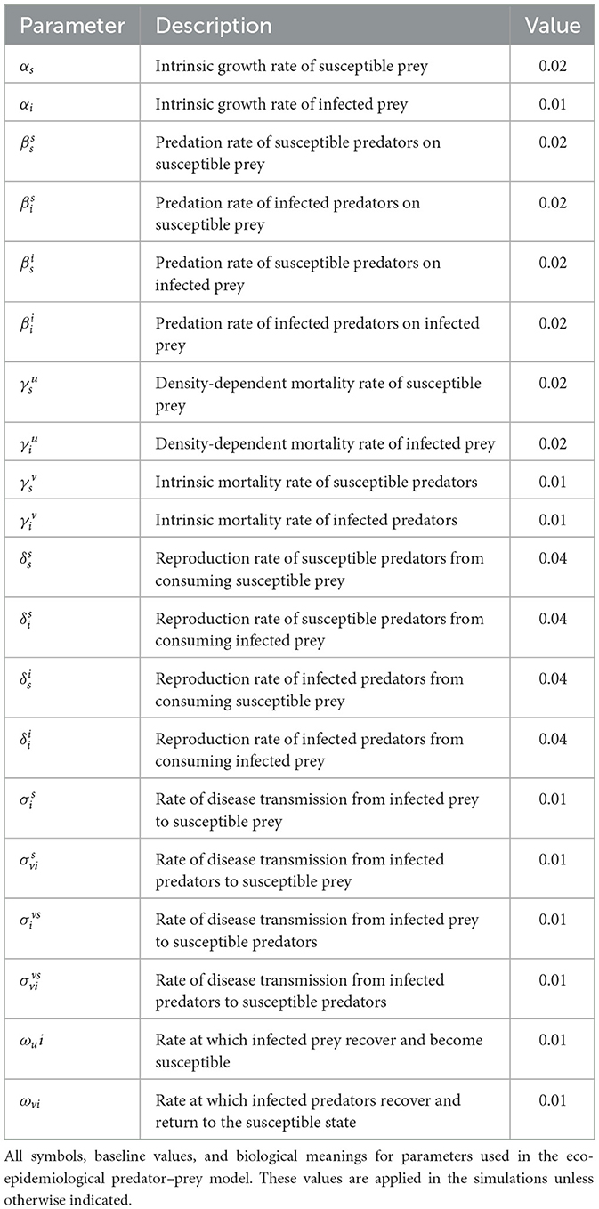
Table 1. Summary of model parameters.

To examine the effect of the initial state of the predator and prey populations on the predator-prey system, we consider two cases:

• Case 1. We fix the susceptible prey initial population at 0.7 and the infected prey initial population at 0.3 while gradually decreasing the ratio of the susceptible predator population from 1 to 0 and increasing the ratio of the infected predator population from 0 to 1

$u_s^0=0.7,u_i^0=1-u_s^0,v_s^0\in \left[0,1\right],v_i^0=1-v_s^0.$

• Case 2. We set the initial populations of susceptible and infected predators at 0.8 and 0.2, respectively. We gradually decrease the proportion of the susceptible prey population from 1 to 0 and increase the ratio of the infected prey population from 0 to 1.

$u_s^0\in \left[0,1\right],u_i^0=1-u_s^0,v_s^0=0.8,v_i^0=1-v_s^0.$

Here $u_s^0$ and $u_i^0$ are the initial population of susceptible and infected prey ($u_s^0+u_i^0=1$ is the total ratio of prey), $v_s^0$ and $v_i^0$ are the initial population of susceptible and infected predators ($v_s^0+v_i^0=1$ is the total ratio of prey).

Figures 1, 2 present the simulation results for the two cases. In Case 1 (Figure 1), the initial prey population is fixed at $(u_s^0,u_i^0)=(0.7,0.3)$, while the ratio of susceptible to infected predators $(v_s^0,v_i^0)$ is varied. In Case 2 (Figure 2), the predator initial condition is fixed at $(v_s^0,v_i^0)=(0.8,0.2)$, and the initial prey composition is varied. Each subplot in both figures illustrates the time evolution of the system over a 250-month period. Across all simulations, the system exhibits transient oscillatory behavior followed by convergence to a steady state, regardless of the initial infection levels. In Figure 1, increasing the proportion of initially infected predators intensifies early fluctuations but does not affect the long-term equilibrium. The predator population stabilizes with approximately 75% susceptible individuals, while the prey population stabilizes at about 50% susceptible. This indicates that the initial infection burden among predators influences only short-term dynamics, with no lasting impact on the final population distributions. Similarly, Figure 2 shows that variations in the initial ratio of susceptible to infected prey primarily affect the speed of disease spread and the amplitude of early oscillations. As the initial infection level in prey increases, infected individuals dominate more quickly; however, the system still converges to a stable coexistence of susceptible and infected individuals in both prey and predator populations. Notably, infected prey persist in all cases, and this suggest that disease becomes endemic in the prey population. These results suggest that the system is resilient to initial infection levels, with disease persisting endemically in both prey and predator populations. The initial distribution of infection affects only short-term dynamics, while long-term outcomes are determined by the intrinsic parameters of the model.

Figure 1

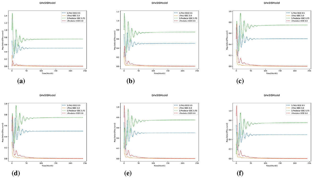
Figure 1. Case 1 with $(u_s^0,u_i^0)=(0.7,0.3)$ and varying initial ratios of susceptible to infected predators $(v_s^0,v_i^0)$. (a) $(v_s^0,v_i^0)=(1,0)$. (b) $(v_s^0,v_i^0)=(0.9,1)$. (c) $(v_s^0,v_i^0)=(0.8,0.2)$. (d) $(v_s^0,v_i^0)=(0.5,0.5)$. (e) $(v_s^0,v_i^0)=(0.3,0.7)$. (f) $(v_s^0,v_i^0)=(0.1,0.9)$.

Figure 2

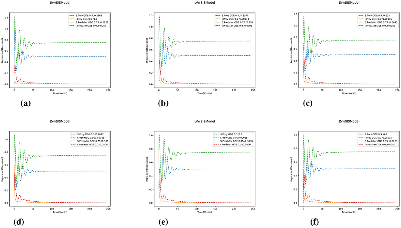
Figure 2. Case 2 with $(v_s^0,v_i^0)=(0.8,0.2)$ and varying initial ratios of susceptible to infected prey $(u_s^0,u_i^0)$. (a) $(u_s^0,u_i^0)=(1,0)$. (b) $(u_s^0,u_i^0)=(0.8,0.2)$. (c) $(u_s^0,u_i^0)=(0.7,0.3)$. (d) $(u_s^0,u_i^0)=(0.4,0.6)$. (e) $(u_s^0,u_i^0)=(0.2,0.8)$. (f) $(u_s^0,u_i^0)=(0,1)$.

4.1 Test 1. Effects of varying predator-prey parameters on the model

To investigate the impact of key parameters on the dynamics of the epidemic in a predator-prey system, we vary the growth, mortality, predation, and reproduction rates under a fixed initial condition for each population. The initial population composition is fixed as follows:

$(u_s^0,u_i^0)=(0.7,0.3),(v_s^0,v_i^0)=(0.8,0.2).$

Here we have 70 % susceptible prey, 30% infected prey, 80% susceptible predators, and 20% infected predators.

We consider three test cases related to the variations of predation and reproduction rates:

• Test 1a. We keep the predation and reproduction rates

${\tilde{\beta }}_g^f={\beta }_g^f,{\tilde{\delta }}_g^f={\delta }_g^f,f=u,vg=s,i,$

while varying birth and death rates.

• Test 1b. We keep the predation and reproduction rates

${\tilde{\beta }}_g^f=0.8{\beta }_g^f,{\tilde{\delta }}_g^f=0.8{\delta }_g^f,f=u,vg=s,i,$

while varying birth and death rates.

• Test 1c. We keep the predation and reproduction rates

${\tilde{\beta }}_g^f=1.2{\beta }_g^f,{\tilde{\delta }}_g^f=1.2{\delta }_g^f,f=u,vg=s,i,$

while varying birth and death rates.

To vary birth and death rates, we multiply given values by P and Q

${\tilde{\alpha }}_g^f=P{\alpha }_g^f,{\tilde{\gamma }}_g^f=Q{\gamma }_g^f,f=u,vg=s,i,$

with P = 0.8, 1, 1.2 and Q = 0.8, 1, 1.2. Here ${\alpha }_g^f$ and ${\gamma }_g^f$ are the growth and mortality rates of prey (f = u) and predator (f = v), where g = s, i corresponds to the susceptible and infected population. The values for ${\alpha }_g^f$, ${\beta }_g^f$, ${\gamma }_g^f$ and ${\delta }_g^f$, as well as transmission and recovery rates, are given in Table 1.

Figures 3–5 depicts the simulation results under varying growth (P) and mortality (Q) rates, as well as different scaling of predation and reproduction rates. The center plot of Figure 3 shows the baseline case where the proportion of susceptible prey begins at 70% and stabilizes around 50%, while the population of susceptible predators starts at 80% and settles at approximately 75%. When the mortality rate increases for all species, only the susceptible prey population increases while the number of susceptible predators decreases, indicating a distinct behavioral shift within the ecosystem. Conversely, decreasing the mortality rate leads to a slight increase in the susceptible predator ratio, but both prey ratios fall below their initial values, and the system takes longer to reach equilibrium.

Figure 3

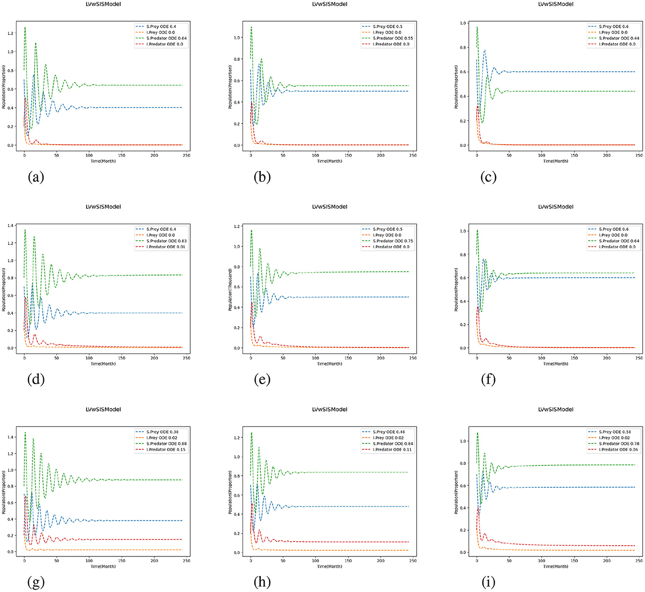
Figure 3. Test 1a: Effects of scaling growth and mortality rates. We use $({\tilde{\beta }}_g^f,{\tilde{\delta }}_g^f)=({\beta }_g^f,{\delta }_g^f)$ for predation and reproduction, and ${\tilde{\alpha }}_g^f=P{\alpha }_g^f$ and ${\tilde{\gamma }}_g^f=Q{\gamma }_g^f$ for growth and mortality. (a) (P, Q) = (0.8, 0.8). (b) (P, Q) = (0.8, 1.0). (c) (P, Q) = (0.8, 1.2). (d) (P, Q) = (1.0, 0.8). (e) (P, Q) = (1.0, 1.0). (f) (P, Q) = (1.0, 1.2). (g) (P, Q) = (1.2, 0.8). (h) (P, Q) = (1.2, 1.0). (i) (P, Q) = (1.2, 1.2).

Figure 4

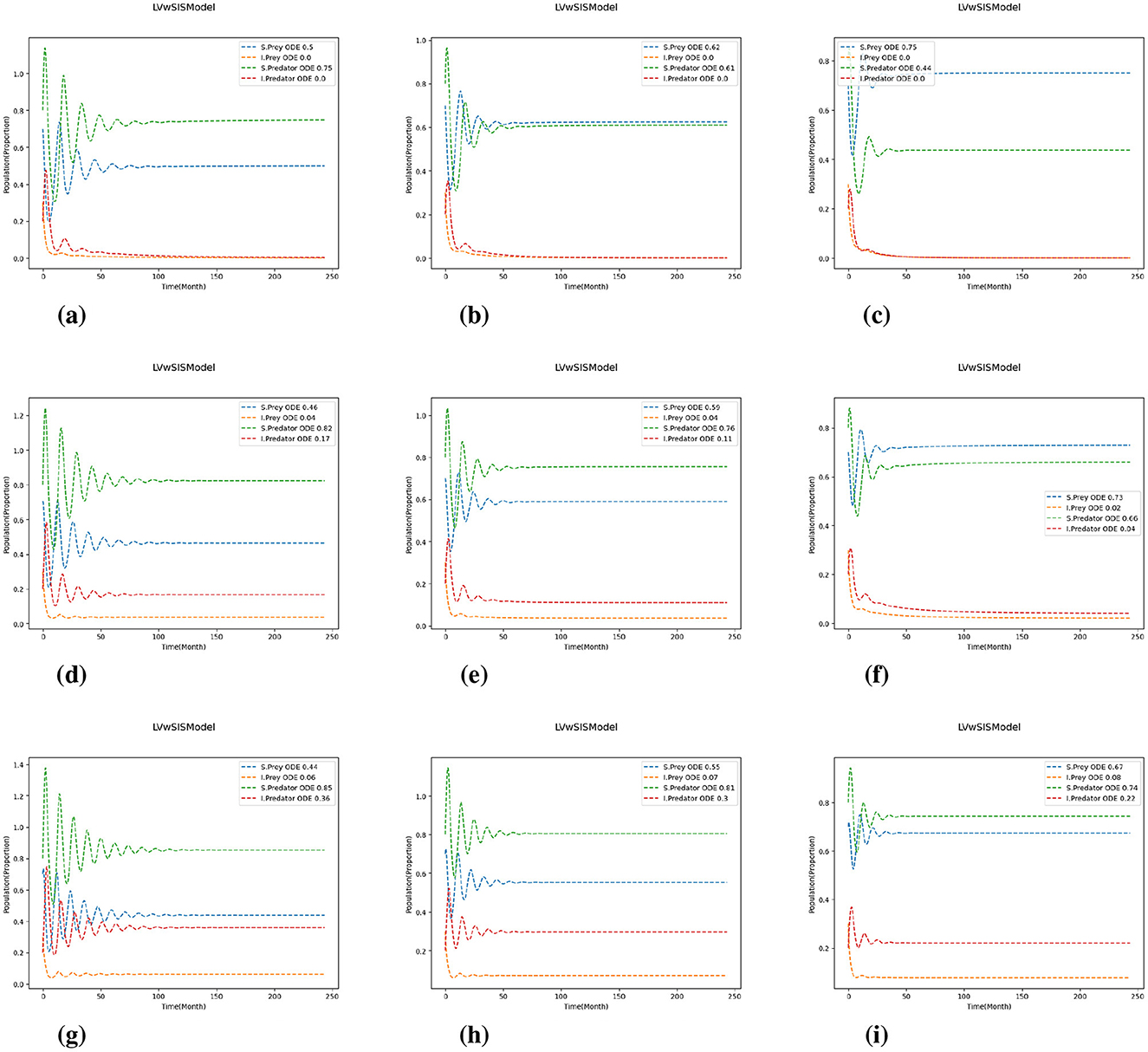
Figure 4. Test 1b with $({\tilde{\beta }}_g^f,{\tilde{\delta }}_g^f)=0.8\times ({\beta }_g^f,{\delta }_g^f)$ for predation and reproduction rates. The results are shown for varying values of P and Q: ${\tilde{\alpha }}_g^f=P{\alpha }_g^f$ and ${\tilde{\gamma }}_g^f=Q{\gamma }_g^f$ for growth and mortality rates. (a) (P, Q) = (0.8, 0.8). (b) (P, Q) = (0.8, 1.0). (c) (P, Q) = (0.8, 1.2). (d) (P, Q) = (1.0, 0.8). (e) (P, Q) = (1.0, 1.0). (f) (P, Q) = (1.0, 1.2). (g) (P, Q) = (1.2, 0.8). (h) (P, Q) = (1.2, 1.0). (i) (P, Q) = (1.2, 1.2).

Figure 5

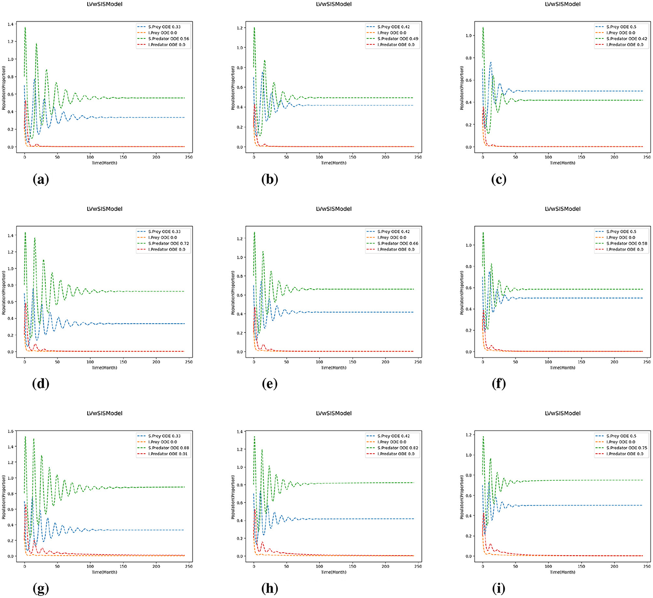
Figure 5. Test 1c with $({\tilde{\beta }}_g^f,{\tilde{\delta }}_g^f)=1.2\times ({\beta }_g^f,{\delta }_g^f)$ for predation and reproduction rates. The results are shown for varying values of P and Q: ${\tilde{\alpha }}_g^f=P{\alpha }_g^f$ and ${\tilde{\gamma }}_g^f=Q{\gamma }_g^f$ for growth and mortality rates. (a) (P, Q) = (0.8, 0.8). (b) (P, Q) = (0.8, 1.0). (c) (P, Q) = (0.8, 1.2). (d) (P, Q) = (1.0, 0.8). (e) (P, Q) = (1.0, 1.0). (f) (P, Q) = (1.0, 1.2). (g) (P, Q) = (1.2, 0.8). (h) (P, Q) = (1.2, 1.0). (i) (P, Q) = (1.2, 1.2).

Comparing the different scaling cases in Figures 4, 5, it is evident that a change in predation and reproduction rates further influences these dynamics. When these rates are reduced (Figure 4), the system exhibits more stability, with rapidly damping oscillations and faster equilibrium by the populations. In contrast, increasing predation and reproduction rates (Figure 5) result in larger, more persistent oscillations and delayed stabilization, emphasizing the destabilizing effects of increased biological activity. Notably, in all cases, the magnitude of population change is influenced by the difference between the growth and mortality scaling factors (P and Q); larger discrepancies (P>Q) lead to more pronounced changes. The proportion of infected predators rises substantially with increasing birth rates, especially when the birth rate coefficient exceeds the death rate coefficient, while the infected prey population typically declines toward zero. These results indicate that higher predation and reproduction rates destabilize populations, increasing the risk of fluctuations and collapse. In contrast, reducing these rates or adjusting growth and mortality can enhance stability and resilience. Thus, interventions targeting these parameters, such as predator management or habitat modification, can play a critical role in maintaining ecosystem health.

4.2 Test 2. Effects of varying epidemic parameters on the model

Next, we modify the coefficients of the transmission and recovery rate to investigate their influence on the dynamics of the predator-prey system (Figure 6). As before, the values for ${\tilde{\sigma }}_g^f=P{\sigma }_g^f$ and ${\tilde{\omega }}_g^f=Q{\omega }_g^f$ are set to 1, 0.8, and 1.2, respectively, with all other parameters given in Table 1.

Figure 6

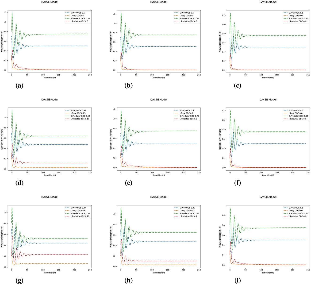
Figure 6. 2, 1.2). Test 2. The results are represented for varying values of T and R, ${\tilde{\sigma }}_g^f=T{\sigma }_g^f$ and ${\tilde{\omega }}_g^f=R{\omega }_g^f$ for the transmission and recovery rates. (a) (T, R) = (0.8, 0.8). (b) (T, R) = (0.8, 1.0). (c) (T, R) = (0.8, 1.2). (d) (T, R) = (1.0, 0.8). (e) (T, R) = (1.0, 1.0). (f) (T, R) = (1.0, 1.2). (g) (T, R) = (1.2, 0.8). (h) (T, R) = (1.2, 1.0). (i) (T, R) = (1.2, 1.2).

The results reveal that when P>Q, indicating that growth rates exceed mortality rates, infected populations–particularly infected predators–experience substantial growth due to increased exposure to infected prey. This dynamic highlights the role of ecological scaling in amplifying infection intensity. Interestingly, variations in transmission and recovery rates do not significantly affect the time required for the system to reach equilibrium. While higher transmission relative to recovery increases infection prevalence, especially among predators, the overall time to stabilization remains largely unchanged. These findings suggest that although infection intensity is sensitive to epidemiological parameters, the system exhibits a form of ecological resilience: long-term stability is preserved despite fluctuations in disease burden. This robustness implies that managing ecological parameters such as growth and predation may be more effective for influencing system stability than targeting transmission or recovery alone.

4.3 Test 3. Effect of varying diffusion

We solve a system of four coupled reaction-diffusion equations and conduct numerical simulations under three diffusion cases: Base, Low, and Lower. In each case, we assign unique diffusion coefficients to the four population classes: susceptible prey (d_us), infected prey (d_ui), susceptible predators (d_vs), and infected predators (d_vi). All other model parameters and initial conditions remain fixed throughout the simulations. The diffusion cases are defined such that each successive case reduces the diffusion coefficients by a factor of 10 compared to the previous one. Specifically, we consider the following:

• Base: $d_{u_s}=10^{-3}$, $d_{u_i}=10^{-4}$, $d_{v_s}=10^{-4}$, $d_{v_i}=10^{-5}$

• Low diffusion: $d_{u_s}=10^{-4}$, $d_{u_i}=10^{-5}$, $d_{v_s}=10^{-5}$, $d_{v_i}=10^{-6}$

• Lower diffusion: $d_{u_s}=10^{-5}$, $d_{u_i}=10^{-6}$, $d_{v_s}=10^{-6}$, $d_{v_i}=10^{-7}$

Results are presented for the averages over the domain and numerical solution profiles at different time steps, illustrating the influence of diffusion on the spatio-temporal dynamics of predator–prey–infection interactions. The results demonstrate how variations in diffusion rates shape spatial distribution, affect population dynamics, and influence the alignment between predator and prey populations in different diffusion cases.

Figure 7 displays the average population dynamics in the spatio-temporal model under varying diffusion values and spatial resolutions. The six subplots are arranged in two rows to illustrate how varying spatial resolution (Nx = Ny) and diffusion rates impact the average population. The upper row represents the impact of spatial resolution on the average population, while the lower row shows the effect of diffusion. More specifically, each subplot tracks the temporal behavior of the four populations: susceptible prey (dotted red), infected prey (solid blue), susceptible predators (dashed orange), and infected predators (dashed green). Figures 7a–c present results for increasing spatial resolutions N_x = N_y = 10, 20, and 40, respectively, while each plot includes the three diffusion cases. Each plot in the top row explicitly compares these diffusion variations, displaying how different diffusion rates (represented by solid lines for higher, dashed lines for lower, and dotted lines for the lowest diffusion) affect population and stabilization times. Lower diffusion rates consistently result in longer-lasting and larger oscillations before stabilization compared to higher diffusion rates. Furthermore, this effect is increasingly evident as spatial resolution increases from 10 to 40, with clearer and more extended transient dynamics becoming apparent at finer resolutions. Across these plots, the overall oscillatory patterns remain relatively consistent, with similar amplitudes and periods of oscillation. Although increasing spatial resolution introduces subtle refinements in the shape and timing of the oscillations, the broad qualitative dynamics, such as the frequency and magnitude of population cycles, remain largely unchanged. Thus, under moderate diffusion, spatial resolution has a limited impact on the global average dynamics, primarily influencing fine-scale details rather than the overall system behavior. The plots in the Figures 7d–f highlight the effects of decreasing diffusion across the same spatial resolutions. As diffusion decreases from Figures 7d–f, the system exhibits fewer oscillations in the susceptible prey and predator populations. In the lower case (Figure 7f), the dynamics are relatively smooth and converge quickly to equilibrium. However, in the low diffusion case (Figure 7e), oscillations become more sustained, with slow convergence, and in the base diffusion case (Figure 7d), these effects are amplified. This progression demonstrates a lower diffusion reduces the rate of spatial mixing. In summary, diffusion strength plays a central role in shaping the ecological stability and convergence of the predator–prey–infection system. Lower diffusion leads to limited spatial mixing, resulting in faster stabilization and reduced oscillatory behavior. This reflects biological situations where species exhibit low mobility or restricted dispersal, thereby reducing contact between prey and predators. In contrast, higher diffusion increases movement and spatial encounters, sustaining predator-prey interactions and infection spread, and prolonging the transient dynamics of the system. While spatial resolution has a lesser effect on global averages, it refines the accuracy of these dynamics, particularly under low diffusion.

Figure 7

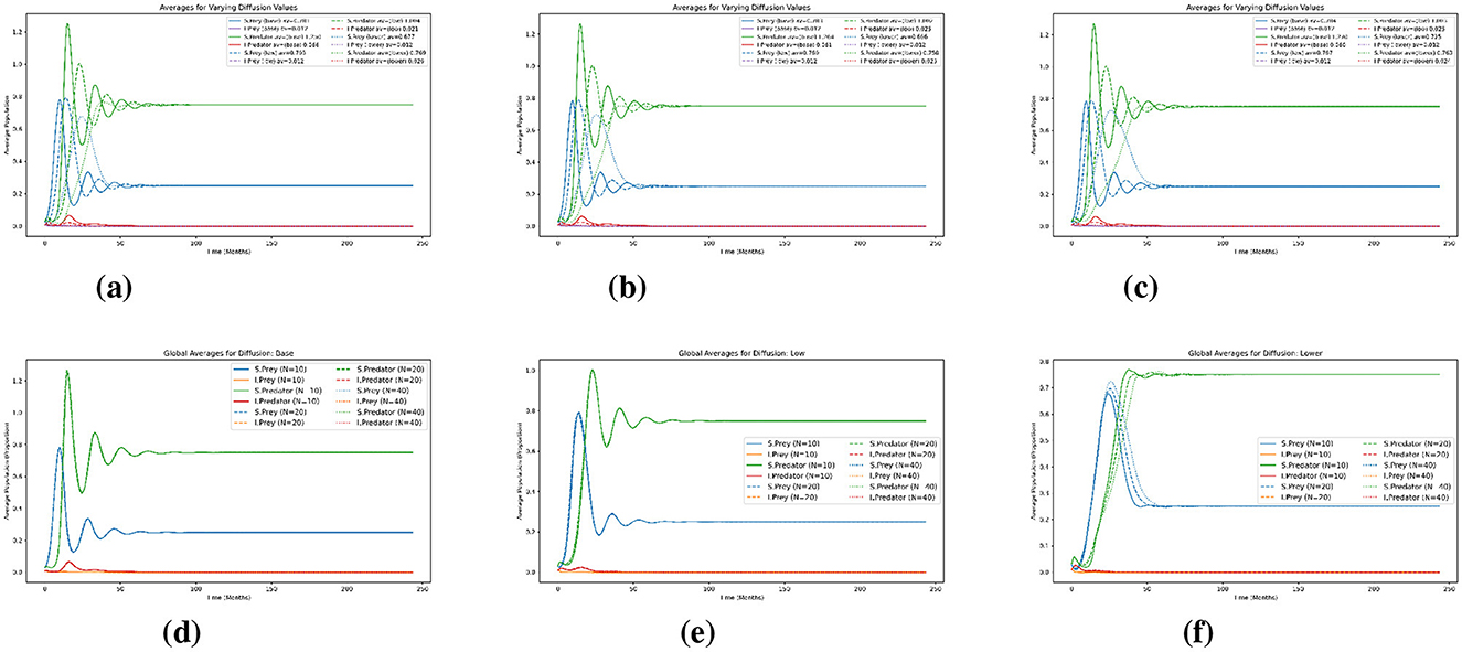
Figure 7. Test 3. Effects of spatial resolution and diffusion on the dynamics of the species in the model. Average population dynamics under three diffusion cases (base, low and lower) on the spatial grids N_x = N_y = 10, 20, 40 in the first row. Each plot shows the temporal evolution of susceptible and infected prey and predator populations. (a) N_x = N_y = 10. (b) N_x = N_y = 20. (c) N_x = N_y = 40. (d) Base. (e) Low. (f) Lower.

Figure 8 presents the solution profile of the spatio-temporal model with the base diffusion case to capture the spatial evolution of the four population categories: susceptible prey (u_s), infected prey (u_i), susceptible predators (v_s) and infected predators (v_i) at selected time steps: 0, 10, 20, 50, and 120 months. Each row corresponds to one population type: (a) susceptible prey, (b) infected prey, (c) susceptible predator, and (d) infected predator, while each column shows the spatial distribution at a given time. At t = 0, all populations are initially localized within a central square region, reflecting a spatially confined initial condition. As time progresses, the diffusion process drives the outward spread of each population. By t = 10 and t = 20 months, the distributions begin to exhibit smooth concentric patterns. Over longer time scales (50–120 months), the system approaches spatial equilibrium, with susceptible populations (u_s) and (v_s) becoming nearly uniform throughout the domain. Infected populations (u_i) and (v_i) exhibit a more transient behavior. Infected prey densities increase initially but begin to decrease significantly by t = 50, while infected predators are nearly extinguished by t = 120. These trends are consistent with the dynamics of a disease in which the infection is temporary and eventually fades as the system stabilizes. In particular, the susceptible predator population tends to concentrate in regions with higher prey density, and this reflects spatial predator-prey coupling. Thus, the base diffusion case enables moderate spatial mixing, leading to the formation of structured yet stable spatial patterns that reflect the interplay between infection dynamics and ecological interactions.

Figure 8

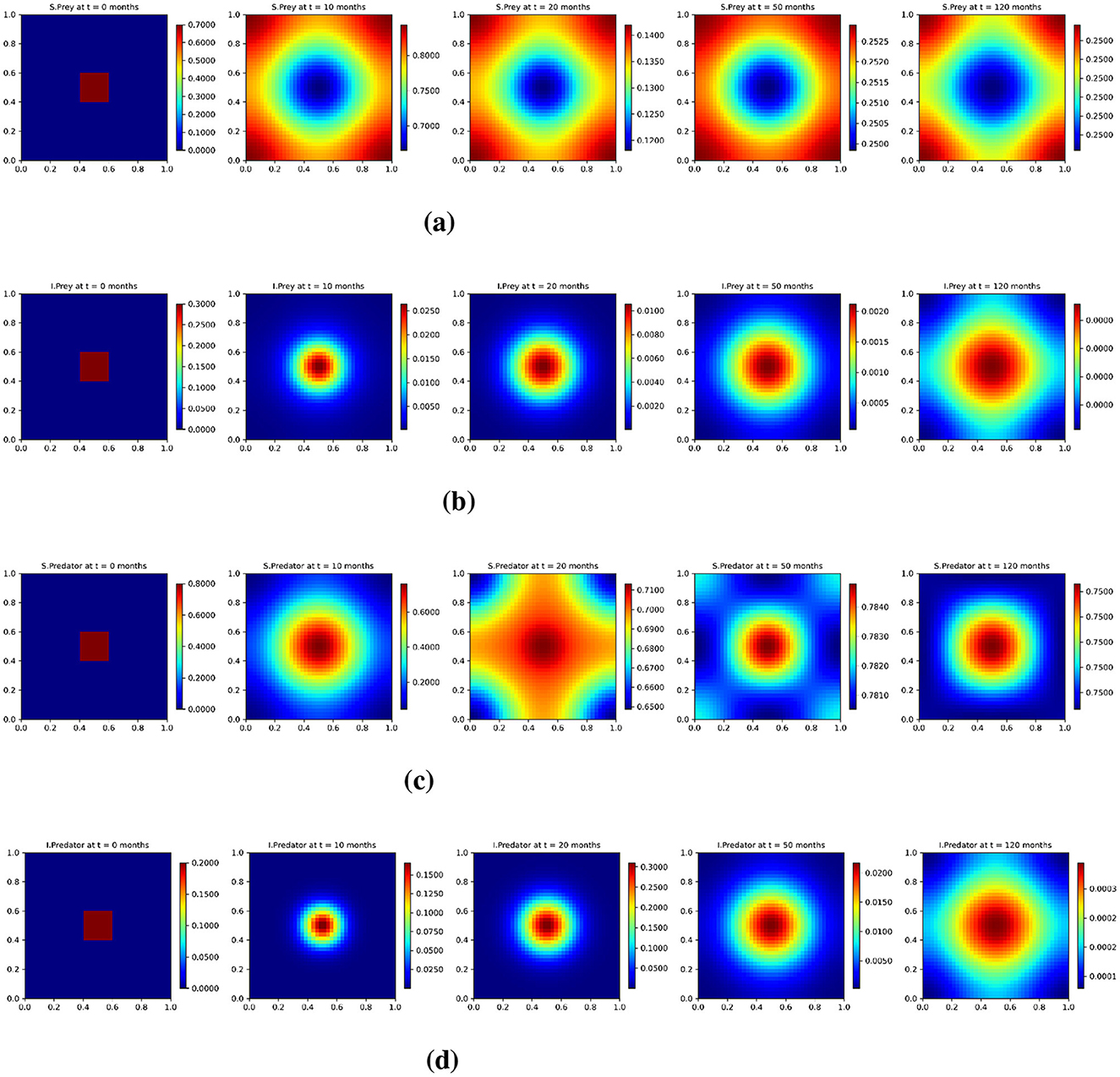
Figure 8. Test 3. Solution profiles of the spatio-temporal eco-epidemiological model at different time steps with the base diffusion coefficients. (a) Susceptible prey population (u_s); (b) infected prey population (u_i); (c) susceptible predator population (v_s); (d) infected predator population (v_i). Profiles are shown across a 2D domain over five selected time points: t = 0, t = 10, t = 20, t = 50, and t = 120 months.

Similarly, in Figure 9, we present the spatial evolution of each population group under the low diffusion scenario in the spatio-temporal model at selected time points: 0, 10, 20, 50, and 120 months. The rows correspond to (a) susceptible prey (u_s), (b) infected prey (u_i), (c) susceptible predator (v_s), and (d) infected predator (v_i). At the initial time (t = 0), all populations are confined to a central region, reflecting a localized initial condition. Due to the reduced diffusion rates, the species spread more slowly compared to the base scenario. This is evident in the snapshots at t = 10 and t = 20 months, where population densities remain sharply localized with steep spatial gradients, and ring-like diffusion patterns emerge slower. As time progresses, the system moves toward homogenization, but the transition is significantly slower than in the base case. By t = 50 and t = 120 months, infected prey and predator populations still exhibit a recognized spatial structure, and this indicates a longer persistence infection and a less uniform spread. Susceptible populations also display more pronounced patchiness and high-density regions remain spatially confined rather than diffusing evenly across the domain. These effects are particularly noticeable in the infected compartments, where the clusters remain sharper and more localized than in the base diffusion case. This slower spatial mixing under low diffusion supports the earlier observation that reduced diffusion prolongs transient dynamics, delays convergence to equilibrium, and allows local population heterogeneity to persist. The spatial dynamics remain uneven throughout the simulation period, highlighting the role of diffusion as a key mechanism for smoothing gradients and accelerating ecological stabilization.

Figure 9

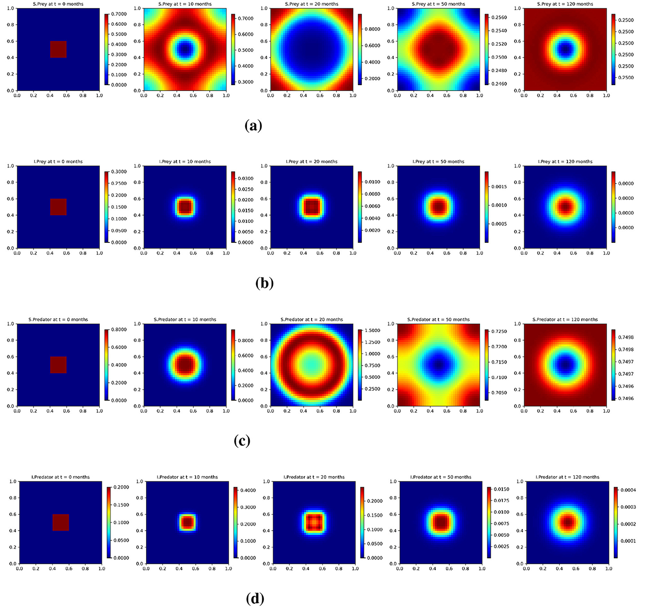
Figure 9. Test 3. Solution profiles of the spatio-temporal eco-epidemiological model at different time steps with the low diffusion coefficients. (a) Susceptible prey population (u_s); (b) Infected prey population (u_i); (c) Susceptible predator population (v_s); (d) Infected predator population (v_i). Profiles are shown across a 2D domain over five selected time points: t = 0, t = 10, t = 20, t = 50, and t = 120 months.

Furthermore, the results for the lower diffusion case are shown in Figure 10 and follow the same presentation style as the base and low diffusion cases. At t = 0, all populations are initially confined to a central region, reflecting a localized starting condition. Due to the significantly reduced diffusion rate, spatial spread is highly restricted throughout the simulation. Unlike in the base or low diffusion cases, the populations remain tightly clustered for extended periods. Snapshots at t = 10 and t = 20 months reveal sharply localized density peaks and steep spatial gradients, particularly in the infected populations. Even at t = 50 and t = 120 months, only limited outward diffusion has occurred, and strong spatial heterogeneity persists in all populations.

Figure 10

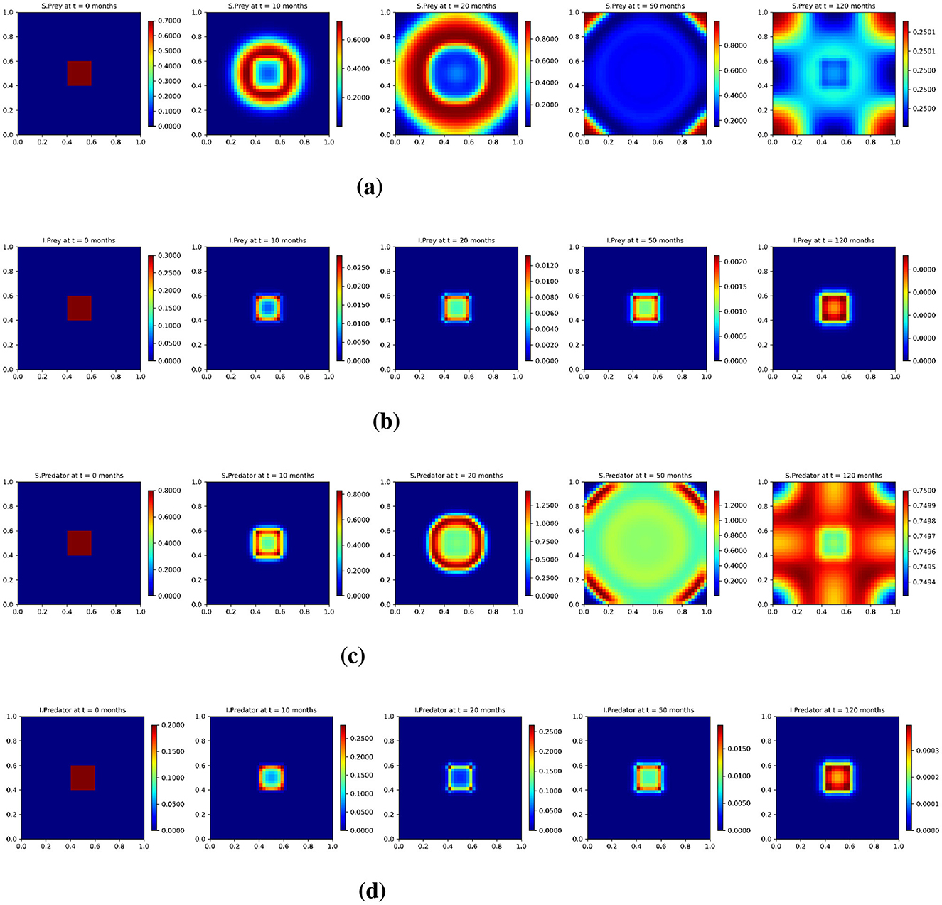
Figure 10. Test 3. Solution profiles of the spatio-temporal eco-epidemiological model at different time steps with the lower diffusion coefficients. (a) Susceptible prey population (u_s); (b) Infected prey population (u_i); (c) Susceptible predator population (v_s); (d) Infected predator population (v_i). Profiles are shown across a 2D domain over five selected time points: t = 0, t = 10, t = 20, t = 50, and t = 120 months.

Figure 11 displays the one-dimensional cross-sectional density profiles of the four species populations with diffusion model, susceptible prey (u_s), infected prey (u_i), susceptible predator (v_s), and infected predator (v_i) along the horizontal axis x∈[0, 1], taken at five time points: 0, 10, 20, 50, and 120 months. Each subplot compares the density curves of the four populations, with solid blue for u_s, dashed red for u_i, dash-dotted green for v_s, and dotted orange for (v_i). The rows (a), (b), and (c) correspond to mesh sizes 10, 20 and 40 respectively. Susceptible prey and predator populations show a broad spread and sustained concentrations at intermediate times (e.g., 20–50 months). In contrast, infected populations show a pattern of increase and decrease, they grow initially, peak, and then decline. By t = 120 months, both the infected prey and predator densities have a long-term decline in the disease.

Figure 11

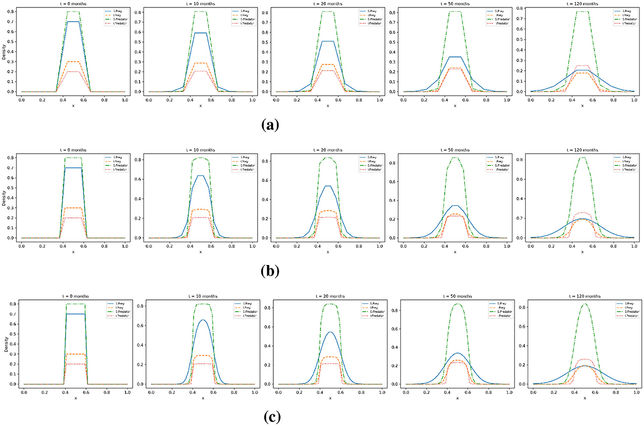
Figure 11. Horizontal cross-sectional density profiles along the x-axis for all species with the base diffusion coefficients. (a) Mesh resolution N_x = N_y = 10; (b) mesh resolution N_x = N_y = 20; (c) mesh resolution N_x = N_y = 40. The profiles are shown over five selected time points: t = 0, t = 10, t = 20, t = 50, and t = 120 months.

4.3.1 Biological interpretation summary

Our numerical results reveal that while initial infection conditions influence early dynamics, they do not alter long-term ecological outcomes. Regardless of the initial proportion of infected prey and predators, the system consistently converges to a stable coexistence equilibrium. This suggests that the predator–prey–infection system exhibits ecological resilience to the severity of initial outbreaks. In contrast, variations in ecological and epidemiological parameters, such as growth, mortality, predation, reproduction, transmission, and recovery rates have a substantial impact on both transient and long-term dynamics. For example, when birth rates exceed mortality rates (P>Q), infected predator populations increase due to greater exposure, while infected prey decline. Elevated predation and reproduction rates destabilize the system, leading to amplified oscillations and delayed stabilization, while lower values promote faster convergence and ecological stability. Similarly, increasing transmission relative to recovery intensifies infection prevalence, particularly among predators, although the time to equilibrium remains largely unaffected. These findings highlight that while infection intensity is sensitive to parameter shifts, the underlying predator–prey dynamics exhibits robust long-term stability. Spatial processes further shape ecological outcomes. Moderate diffusion facilitates spatial mixing, supporting predator–prey coexistence and eventual infection fadeout. In contrast, limited diffusion restricts movement, prolongs transients, and leads to persistent infection pockets and uneven species distributions. Cross-sectional profiles reinforce these patterns, showing that susceptible populations spread more uniformly, while infected populations form sharp transient peaks. These results underscore the ecological importance of species mobility in regulating contact rates, infection persistence, and the emergence of spatially structured equilibrial. Together, these insights suggest that managing ecological parameters and promoting appropriate levels of species mobility could be key strategies for controlling disease spread and maintaining ecosystem stability in spatially structured environments.

5 Conclusion

The epidemic dynamics in the spatio-temporal predator-prey model are derived by combining two models: the SIS epidemic model and the Lotka-Volterra (LV) predator-prey model. We simulated a system of four ordinary differential equations and obtained numerical results using the Euler method.

First, we examined how the initial conditions of each population class affect the system. Our main finding is that the initial ratios of susceptible to infected prey and predators influence the time required to reach a steady state. Although the system consistently converges to the same equilibrium, the time to stabilization depends on the initial deviation from that equilibrium. Although these differences are subtle, the pattern is clear: the greater the deviation, the longer the system takes to stabilize.

Second, we explored the impact of key parameters on system stability. The results show that a higher mortality rate accelerates convergence to the steady state. An increased growth rate primarily contributes to the growth of the infected predator population more than the susceptible predators, while the prey population may decline due to intensified predation pressure. In addition, when the death rate surpasses the birth rate, the ratio of susceptible prey exceeds that of susceptible predators. These findings underscore the sensitivity of population dynamics to ecological and epidemiological parameters.

Finally, we investigated the effect of diffusion by varying the diffusion coefficients while keeping all other parameters fixed. Diffusion plays a key role in shaping the dynamics of the spatio-temporal model. Higher diffusion leads to faster spatial mixing and faster stabilization, whereas lower diffusion slows population spread, prolongs infection persistence, and maintains spatial heterogeneity. These results highlight the importance of diffusion in determining how quickly and uniformly the system approaches equilibrium. As a natural extension of this work, the model could be enhanced by incorporating additional ecological complexities, such as seasonal variations, heterogeneous landscapes, or predator-prey preference dynamics. Investigating stochastic versions of the model may also offer valuable insights into the role of randomness in disease persistence and extinction. Furthermore, the use of more advanced numerical methods or adaptive mesh refinement techniques could improve accuracy in low-diffusion regimes and help mitigate the numerical stiffness observed in the simulations.

Data availability statement

The original contributions presented in the study are included in the article/supplementary material, further inquiries can be directed to the corresponding author.

Author contributions

HJ: Writing – original draft, Investigation, Writing – review & editing, Conceptualization. MV: Validation, Project administration, Investigation, Supervision, Writing – original draft, Writing – review & editing, Methodology, Conceptualization. NM: Validation, Writing – review & editing, Investigation, Visualization. AS: Supervision, Conceptualization, Writing – review & editing, Project administration, Funding acquisition.

Funding

The author(s) declare that no financial support was received for the research and/or publication of this article.

Conflict of interest

The authors declare that the research was conducted in the absence of any commercial or financial relationships that could be construed as a potential conflict of interest.

The author(s) declared that they were an editorial board member of Frontiers, at the time of submission. This had no impact on the peer review process and the final decision.

Generative AI statement

The author(s) declare that no Gen AI was used in the creation of this manuscript.

Publisher's note

All claims expressed in this article are solely those of the authors and do not necessarily represent those of their affiliated organizations, or those of the publisher, the editors and the reviewers. Any product that may be evaluated in this article, or claim that may be made by its manufacturer, is not guaranteed or endorsed by the publisher.

References

1. Montévil M. A primer on mathematical modeling in the study of organisms and their parts. In:Bizzarri M, , editor. Systems Biology. New York, NY: Springer (2018). p. 41–55. doi: 10.1007/978-1-4939-7456-6_4

PubMed Abstract | Crossref Full Text | Google Scholar

2. Swailem M, Täuber UC. Lotka-Volterra predator-prey model with periodically varying carrying capacity. arXiv. (2022). [Preprint]. arXiv:2211.09276. doi: 10.48550/arXiv.2211.09276

Crossref Full Text | Google Scholar

3. Kuhl E, editors. The classical SIS model. In: Computational Epidemiology. Cham: Springer (2021). p. 33–40. doi: 10.1007/978-3-030-82890-5_2

Crossref Full Text | Google Scholar

4. Shaikhet L, Korobeinikov A. Asymptotic properties of the Lotka–Volterra competition and mutualism model under stochastic perturbations. Math Med Biol. (2024) 41:19–34. doi: 10.1093/imammb/dqae001

PubMed Abstract | Crossref Full Text | Google Scholar

5. Davis JD, Olivença DV, Brown SP, Voit EO. Methods of quantifying interactions among populations using Lotka-Volterra models. Front Syst Biol. (2022) 2:1021897. doi: 10.3389/fsysb.2022.1021897

Crossref Full Text | Google Scholar

6. Lahrouz A, Settati A, Akharif A. Effects of stochastic perturbation on the SIS epidemic system. J Math Biol. (2017) 74:469–98. doi: 10.1007/s00285-016-1033-1

PubMed Abstract | Crossref Full Text | Google Scholar

7. Gray A, Greenhalgh D, Hu L, Mao X, Pan J. Stochastic SIS epidemic models with a finite population. Math Biosci. (2011) 232:111–20. doi: 10.1137/10081856X

Crossref Full Text | Google Scholar

8. Pastor-Satorras R, Castellano C, Van Mieghem P, Vespignani A. Epidemic processes in complex networks. Rev Mod Phys. (2015) 87:925. doi: 10.1103/RevModPhys.87.925

Crossref Full Text | Google Scholar

9. Lei C, Han X. Complex dynamics in a discrete eco-epidemiological model with fatal disease in the prey. Qual Theory Dyn Syst. (2025) 24:124. doi: 10.1007/s12346-025-01285-z

Crossref Full Text | Google Scholar

10. Hadeler KP, Freedman HI. Predator-prey populations with parasitic infection. J Math Biol. (1989) 27:609–31. doi: 10.1007/BF00276947

PubMed Abstract | Crossref Full Text | Google Scholar

11. Venturino E. Epidemics in predator-prey models: disease in the predators. Math Med Biol. (2002) 19:185–205. doi: 10.1093/imammb/19.3.185

Crossref Full Text | Google Scholar

12. Mondal B, Sarkar A, Sk N. Treatment of infected predators under the influence of fear-induced refuge. Sci Rep. (2023) 13:16623. doi: 10.1038/s41598-023-43021-0

PubMed Abstract | Crossref Full Text | Google Scholar

13. Mitchinson A. Bacterial Prey Turns the Tables on Predator. London: Nature Publishing Group UK. (2024). doi: 10.1038/d41586-024-00228-z

PubMed Abstract | Crossref Full Text | Google Scholar

14. Gómez-Hernández EA, Moreno-Gómez FN, Córdova-Lepe F, Bravo-Gaete M, Velásquez NA, Benítez HA. Eco-epidemiological predator-prey models: a review of models in ordinary differential equations. Ecol Complex. (2024) 57:101071. doi: 10.1016/j.ecocom.2023.101071

Crossref Full Text | Google Scholar

15. Majee S, Jana S, Kar T, Anand R, Ramprabhakar J. Impact of incubation and gestation periods on the dynamics of a spatially heterogeneous eco-epidemiological model. Sci Rep. (2025) 15:19661. doi: 10.1038/s41598-025-02778-2

PubMed Abstract | Crossref Full Text | Google Scholar

16. Davydovych V, Dutka V, Cherniha R. Reaction–diffusion equations in mathematical models arising in epidemiology. Symmetry. (2023) 15:2025. doi: 10.3390/sym15112025

Crossref Full Text | Google Scholar

17. Naz R, Torrisi M. Closed-form solutions of a reaction–diffusion SIS epidemic model via Lie symmetry analysis. Mathematics. (2024) 12:23. doi: 10.3390/sym16080948

Crossref Full Text | Google Scholar

18. Hu G, Li X, Wang Y. Pattern formation and spatiotemporal chaos in a reaction-diffusion predator-prey system. Nonlinear Dyn. (2015) 81:265–75. doi: 10.1007/s11071-015-1988-2

Crossref Full Text | Google Scholar

19. Zhao XQ, Ruan S. Traveling wave solutions for a diffusive SIS epidemic model. Discrete Continuous Dyn Syst Ser B. (2014) 19:1427–44.

Google Scholar

20. Chen X, Wu J. Dynamics of an SIS epidemic patch model with spatial diffusion and heterogeneous transmission. arXiv. (2023). [Preprint]. arXiv:2301.06645. doi: 10.48550/arXiv.2301.06645

Crossref Full Text | Google Scholar

21. Qiao M, Liu A, Foryś U. Qualitative analysis for a reaction-diffusion predator-prey model with disease in the prey species. J Appl Math. (2014) 2014:236208. doi: 10.1155/2014/236208

Crossref Full Text | Google Scholar

22. Ling Z, Zhang L, Lin Z. Turing pattern formation in a predator-prey system with cross diffusion. Appl Math Model. (2014) 38:5022–32. doi: 10.1016/j.apm.2014.04.015

Crossref Full Text | Google Scholar

23. Sun GQ, Jin Z, Li L, Haque M, Li BL. Spatial patterns of a predator-prey model with cross diffusion. Nonlinear Dyn. (2012) 69:1631–8. doi: 10.1007/s11071-012-0374-6

Crossref Full Text | Google Scholar

24. Upadhyay RK, Roy P. Spread of a disease and its effect on population dynamics in an eco-epidemiological system. Commun Nonlinear Sci Numer Simul. (2014) 19:4170–84. doi: 10.1016/j.cnsns.2014.04.016

Crossref Full Text | Google Scholar

25. Upadhyay RK, Parshad RD, Tripathi NM, Mohan N. An eco-epidemiological model with prey-taxis and slow diffusion: global existence, boundedness and novel dynamics. arXiv. (2025) [Preprint]. arXiv:2504.13764. doi: 10.48550/arXiv.2504.13764

Crossref Full Text | Google Scholar

26. Peng R, Salako RB, Wu Y. Spatial profiles of a reaction-diffusion epidemic model with nonlinear incidence mechanism and varying total population. Nonlinearity. (2025) 38:045006. doi: 10.1088/1361-6544/adbba9

Crossref Full Text | Google Scholar

27. Biswas M, Bairagi N. Discretization of an eco-epidemiological model and its dynamic consistency. J Differ Equ Appl. (2017) 23:860–77. doi: 10.1080/10236198.2017.1304544

Crossref Full Text | Google Scholar

28. Liu X, Yang Z. Numerical analysis of a reaction-diffusion susceptible-infected-susceptible epidemic model. Comput Appl Math. (2022) 41:392. doi: 10.1007/s40314-022-02113-9

Crossref Full Text | Google Scholar

29. Sorokin VG, Vyazmin AV. Nonlinear reaction-diffusion equations with delay: partial survey, exact solutions, test problems, and numerical integration. Mathematics. (2022) 10:1886. doi: 10.3390/math10111886

Crossref Full Text | Google Scholar

30. Krebs CJ. Ecology: The Experimental Analysis of Distribution and Abundance. London: Pearson Education (2009).

Google Scholar

31. Murray JD. Mathematical Biology I: An Introduction. Cham: Springer (2002). doi: 10.1007/b98868

Crossref Full Text | Google Scholar

32. Rojas M, Mena-Lorca S. Transmission of disease between predator and prey in a simple ecological model. J Theor Biol. (2018) 439:90–102.

Google Scholar

33. Gog JR, Swinton JP. The role of immunity in the persistence and spread of infectious diseases in wildlife populations. J Theor Biol. (2002) 218:61–73.

Google Scholar

34. Santos EA, Morais DL. SIS epidemic models for prey with immunity loss in predator-prey systems. Math Biosci. (2021) 338:108636.

Google Scholar

35. Bjørnstad ON, Grenfell BT. Noisy clockwork: time series analysis of population fluctuations in animals. Science. (2001) 293:645–50. doi: 10.1126/science.1062226

PubMed Abstract | Crossref Full Text | Google Scholar

36. He D, Li J. Mathematical models of disease spread and management in wildlife populations. Ecol Lett. (2012) 15:1422–9.

Google Scholar

37. Vasilyeva M, Wang Y, Stepanov S, Sadovski A. Numerical investigation and factor analysis of the spatial-temporal multi-species competition problem. arXiv. (2022) [Preprint]. arXiv:2209.02867. doi: 10.48550/arXiv.2209.02867

Crossref Full Text | Google Scholar

38. Vasilyeva M, Sadovski A, Palaniappan D. Multiscale solver for multi-component reaction-diffusion systems in heterogeneous media. J Comput Appl Math. (2023) 427:115150. doi: 10.1016/j.cam.2023.115150

Crossref Full Text | Google Scholar

39. Wang Y, Vasilyeva M, Sadovski A. Prediction of the survival status for multispecies competition system. In: AIP Conference Proceedings, Vol. 2872. Melville, NY: AIP Publishing (2023). doi: 10.1063/5.0164710

Crossref Full Text | Google Scholar

40. Vasilyeva M, Stepanov S, Sadovski A, Henry S. Uncoupling techniques for multispecies diffusion-reaction model. Computation. (2023) 11:153. doi: 10.3390/computation11080153

Crossref Full Text | Google Scholar

41. Vasilyeva M, Coffin RB, Pecher I. Decoupled multiscale numerical approach for reactive transport in marine sediment column. Comput Methods Appl Mech Eng. (2024) 428:117087. doi: 10.1016/j.cma.2024.117087

Crossref Full Text | Google Scholar

42. Vasilyeva M. Implicit-Explicit schemes for decoupling multicontinuum problems in porous media. J Comput Phys. (2024) 519:113425. doi: 10.1016/j.jcp.2024.113425

Crossref Full Text | Google Scholar

43. Vasilyeva M, Vasiliev V, Tyrylgin A. Conservative finite-difference scheme for filtration problems in fractured media. Math Notes NEFU. (2018) 25:84–101. doi: 10.25587/SVFU.2018.100.20556

Crossref Full Text | Google Scholar

44. Vasilyeva M, Krasnikov A, Gajamannage K, Mehrubeoglu M. Multiscale method for image denoising using nonlinear diffusion process: local denoising and spectral multiscale basis functions. arXiv. (2024) [Preprint]. arXiv:2409.15952. doi: 10.48550/arXiv.2409.15952

Crossref Full Text | Google Scholar

45. Vabishchevich PN. Vasil'eva MV. Explicit-implicit schemes for convection-diffusion-reaction problems. Numer Anal Appl. (2012) 5:297–306. doi: 10.1134/S1995423912040027

Crossref Full Text | Google Scholar

46. Allen LJS, van den Driessche P. The basic reproduction number in some discrete-time epidemic models. J Differ Equ Appl. (2008) 14:1127–47. doi: 10.1080/10236190802332308

Crossref Full Text | Google Scholar

47. Smith HL, Waltman P. The Theory of the Chemostat: Dynamics of Microbial Competition. Cambridge Studies in Mathematical Biology. Cambridge: Cambridge University Press (1995).

Google Scholar

48. LeVeque RJ. Finite Difference Methods for Ordinary and Partial Differential Equations: Steady-State and Time-Dependent Problems. Philadelphia, PA: Society for Industrial and Applied Mathematics (SIAM) (2007). doi: 10.1137/1.9780898717839

Crossref Full Text | Google Scholar

49. Hundsdorfer W, Verwer JG. Numerical Solution of Time-Dependent Advection-Diffusion-Reaction Equations, Vol 33 of Springer Series in Computational Mathematics. Berlin: Springer (2003). doi: 10.1007/978-3-662-09017-6

Crossref Full Text | Google Scholar

50. Kot M. Elements of Mathematical Ecology. Cambridge: Cambridge University Press (2001). doi: 10.1017/CBO9780511608520

Crossref Full Text | Google Scholar

Appendix

We introduce the SIS epidemic model, followed by a discussion of the classical LV model. The SIS model describes the spread of infectious diseases within a population where individuals can move between susceptible and infected states, do not develop immunity, and become susceptible again. This model can be used for diseases that do not have long-term immunity, chronic or recurrent infections, or short-lived immunity. The foundation for mathematical epidemiology was presented by describing how infectious diseases spread in a population using differential equations.

The SIS model consists of two nonlinear differential equations that represent the rate of change in the population of susceptible S(t) and infected populations I(t)

$\begin{array}{l}\frac{\partial S}{\partial t}=-\sigma SI+\omega I,\\ \frac{\partial I}{\partial t}=\sigma SI-\omega I,& (21)\end{array}$

where S is the susceptible population, I is the infected population, σ is the infection rate of the susceptible, ω is the recovery rate at which the infected return to the susceptible.

The Lotka-Volterra model is a mathematical framework that describes the dynamics of predator-prey interactions in an ecological system. It consists of a system of coupled differential equations that represent the populations of predators and prey over time. A modified version of the model, based on logistic prey population growth, consists of two nonlinear differential equations that represent the rate of change in the populations of prey u(t) and predator v(t)

$\begin{array}{l}\frac{\partial u}{\partial t}=\alpha u\left(1-\frac{u}{k}\right)-\beta uv,\\ \frac{\partial v}{\partial t}=\delta vu-{\gamma }^{v}v,& (22)\end{array}$

where u is the prey population, v is the predator population, α is the natural birth rate of the prey, k is carrying capacity, β is the predation rate (the rate at which predators consume prey), δ is the predator reproduction rate (conversion of consumed prey into predator offspring) and γ is the natural death rate of predators. In this formulation, the first term in the prey equation represents the logistic growth. When resources are abundant, its population grows rapidly but slowly as it approaches carrying capacity, while the second term captures the predation effect. To simplify the model and explicitly represent the natural mortality of the prey, we replace the logistic term with a simpler quadratic death term γ^u u², where γ accounts for all causes of death that become more significant as the population grows; such as competition for limited resources. This leads to the following system

$\begin{array}{l}\frac{\partial u}{\partial t}=\alpha u-\beta uv-{\gamma }^u{u}^2,\\ \frac{\partial v}{\partial t}=\delta vu-{\gamma }^{v}v.& (23)\end{array}$

The modified formulation removes explicit carrying capacity k and instead assumes that prey mortality increases quadratically with population size. This approach maintains the self-limiting nature of prey growth while allowing a more flexible representation of mortality, which may arise from competition, resource limitation, or other density-dependent factors [31, 50].