Stability and entropy production in fractional bio-heat transport models via generalized (q, τ)-entropy

We propose a novel framework for modeling thermal transport in biological tissues based on a fractional bio-heat diffusion equation regularized by a generalized (q, τ)-entropy functional. The model incorporates a Caputo-Numerical simulations demonstrate the evolution of temperature profiles and entropy dynamics, revealing the interplay between fractional memory, metabolic heat generation, and entropy-induced resistance. A stability theorem this framework offers a physically consistent and flexible approach grounded in non-equilibrium statistical mechanics and bio-thermal regulation, making it suitable for applications in complex biological media with long-range.

1 Introduction

Information theory, statistical mechanics, and thermodynamics are all based on entropy. In systems made up of separate microscopic states, disorder and uncertainty are measured by the classical Boltzmann-Gibbs entropy, which is expressed as S = − ∑p _i log p_i [1–3]. However, as shown in intricate biological, physical, visual, and financial processes, this form is constrained when modeling systems with long-range interactions, memory effects, or anomalous diffusion [4–6]. Several generalized entropy frameworks have been developed to get over these restrictions. Among the most prominent is the Tsallis entropy, which introduces non-extensive behavior and is specified by a deformation parameter q:

$S_q=\frac{1-\sum {\displaystyle p_i^q}}{q-1}.$

This approach has been effectively used to study quantum systems, turbulence, and multifractals. The study of decoherence, entanglement, and instability in quantum systems has been enhanced by the extension of information measures to density matrices and quantum probability spaces due to advancements in quantum entropy. However, as noted in Dingyu and Lu [7] and Agarwal et al. [8], fractional calculus offers a natural instrument to represent dynamics with memory and hereditary features. The Riemann-Liouville, Caputo, and Hadamard kinds of fractional derivatives and integrals extend conventional differential operators and enable the modeling of viscoelastic materials, anomalous diffusion, and sub-diffusive processes. Particularly in the context of stability analysis and entropy-producing systems, the unification of fractional dynamics with non-extensive entropy has garnered interest in recent years [9, 10].

Biological tissues exhibit highly complex thermal behavior, characterized by heterogeneous structure, multiple time scales of heat conduction, and active metabolic heat generation. Classical models based on the Fourier law of heat conduction are limited in this context, as they neglect memory effects and the intrinsic non-equilibrium nature of living tissues. Recent studies have demonstrated that fractional-order diffusion models provide a natural extension of the Pennes bio-heat equation, capturing anomalous thermal transport and sub-diffusive behavior observed in biological systems [11–14]. In this work, we adopt a (q, τ)-entropy framework that extends existing methods by including a scaling parameter τ that modulates the memory kernel of the fractional operator and a deformation parameter q that controls the degree of non-extensivity. This makes it possible to interpret energy dissipation and entropy creation in bio-heat transport in a consistent thermodynamic manner. Our fractional diffusion model's entropy term −λ log _{q, τ}(T) functions as an effective potential, dynamically modifying thermal resistance in response to local temperature variations. This mechanism offers a physically grounded way to regularize thermal transport in complicated biological media and is consistent with the generalized fluctuation-dissipation relations in non-equilibrium statistical mechanics. Our numerical outcomes show that the (q, τ)-entropy framework captures important aspects of bio-thermal dynamics, such as physically realistic entropy decay and entropy-stabilized patterns of temperature. These findings imply that generalized entropy-based statistical mechanics techniques are useful instruments for improving the modeling of bio-heat transfer and associated processes in living systems.

2 Generalized entropy

Definition 2.1 (Generalized ((q, τ)-Entropy). Let p = {p₁, p₂, …, p_n} be a discrete probability distribution such that p_i > 0, $\sum _{i=1}^n{p}_i=1$. The (q, τ)-entropy associated with the distribution p is formulated by (see Figure 1, for various values of τ and q = 0.5)

$S_{q,\tau }(p):=-{\displaystyle \sum _{i=1}^n}{p}_i·{log}_{q,\tau }(p_i),$

where the deformed logarithm log _{q, τ}(x) is given by

${log}_{q,\tau }(x):=\frac{x^{1-q}-1}{1-q}·{\Gamma }_{q,\tau }(x),$

and the (q, τ)-gamma function is defined as (see Figure 2)

${\Gamma }_{q,\tau }(\alpha )={(1-q)}^{1-\alpha }{\displaystyle \prod _{n=0}^{\infty }}\frac{1-q^{\tau (n+1)}}{1-q^{\tau (\alpha +n)}},\text{for }0<q<1,\tau >0.$

Figure 1

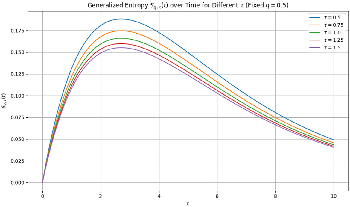
Figure 1. Plot of S_{q, τ}, with q = 0.5 and τ ∈ {0.5, 0.75, 1.0, 1.25, 1.5} respectively. Memory effects lengthen the entropy production process since the entropy decay is slower for greater τ. The degradation is steeper for lower τ because the system recalls previous states more quickly.

Figure 2

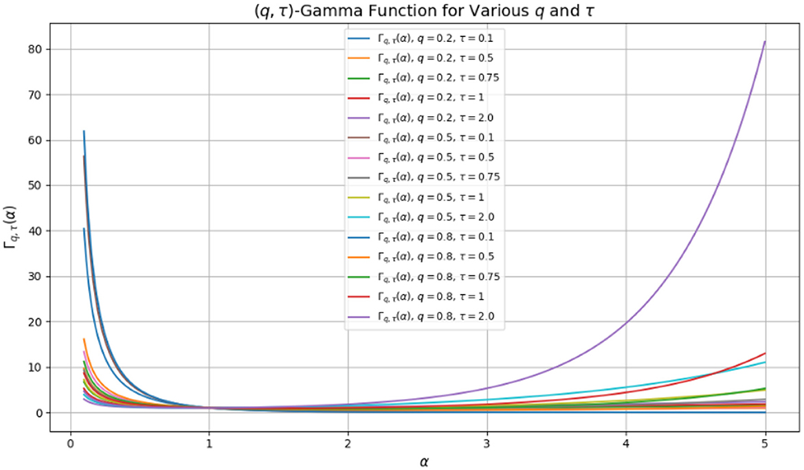
Figure 2. Graph of Γ_{q, τ}(α)for different values of (q, τ).

In the limit (q, τ) → (1,1), this entropy reduces to conventional Shannon entropy and provides a deformation that incorporates scaling tendency and memory [15–17] with its applications in Attiya et al. [18], Alqarni et al. [19], and Hasanov and Yuldashova [20].

2.1 Thermodynamic rationale for the generalized logarithm log_{(q, τ)}(x)

The modified logarithmic function ${log}_{(q,\tau )}(x)=\frac{x^{1-q}-1}{1-q}\times {\Gamma }_{q,\tau }(x)$, which includes a fractional memory kernel Γ_{q, τ}(x), extends the Tsallis-type logarithm. This idea combines the impacts of statistical non-extensive (through the parameter q) with long-range memory or non-locality (via τ), both of which are essential components of thermal transport in intricate and dynamic settings.

2.1.1 From tsallis entropy to fractional memory entropy

In nonextensive thermodynamics, the classical Tsallis logarithm is ${log}_q(x)=\frac{x^{1-q}-1}{1-q},$ which reduces to the natural logarithm known as q → 1. This function basically arises from the maximization of Tsallis entropy and captures the deviation of extensivity due to fractal geometries or long-range connections.

2.1.2 Role of the Γ_{q, τ}(x) term

The historical context of thermal computation in tissue biology reflects the influence of past thermal asserts on current behavior (non-Markovian dynamics), the persistence of temperature distributions over time scales (memory effects), and tissue-specific thermal reactions derived from heterogeneous relaxation times.

2.1.3 Thermodynamic interpretation

The function log_{(q, τ)}(x) could be viewed as a memory-weighted entropy potential. An entropy functional like as S_{q, τ}(f) = −∫f(x) log _{(q, τ)}(f(x))dx, can be used to mimic entropy creation in systems with anomalous, history-dependent behaves, which are prevalent in biological and viscoelastic tissues.

2.1.4 Limit cases

If Γ_{q, τ}(x) → 1, then log_{(q, τ)}(x) → log(x), we can recover the usual logarithm as q → 1. If Γ_{q, τ}(x) encodes power-law decay (as in fractional kernels), then entropy grows in accordance with memory-regulated non-exponential laws (Table 1).

Table 1

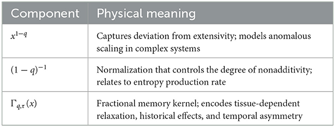
Table 1. Physical interpretation of the terms in log_{(q, τ)}(x).

The (q, τ)-logarithm extends the Tsallis form by including a fractional memory weight, and it is thermodynamical consistent with complex biological systems that have both non-extensivity and long-range memory. This method is necessary to analyze entropy-based occurrences in bio-heat transfer and related fractional diffusion pathways.

Proposition 2.2 ( Basic properties of the (q, τ)-entropy). Let p = {p₁, p₂, …, p_n} be a discrete probability distribution such that p_i > 0 and $\sum _{i=1}^n{p}_i=1$. Define the (q, τ)-entropy as

$S_{q,\tau }(p)=-{\displaystyle \sum _{i=1}^n}{p}_i·{log}_{q,\tau }(p_i),$

where the (q, τ)-logarithm. Then the next properties hold:

(i) Non-negativity: S_{q, τ}(p) ≥ 0, with equality if and only if p_i = 1 for some i and all others zero.

(ii) Maximality at uniform distribution: The entropy S_{q, τ}(p) attains its maximum when $p_i=\frac{1}{n}$ for all i, i.e.,

$S_{q,\tau }(p)\le -{\displaystyle \sum _{i=1}^n}\frac{1}{n}{log}_{q,\tau }\left(\frac{1}{n}\right).$

(iii) Classical limit: In the limit as q → 1, τ → 1, we recover the classical Shannon entropy: $\underset{q\to 1,\tau \to 1}{lim}{S}_{q,\tau }(p)=-\sum _{i=1}^n{p}_{i}log(p_i).$

Proof. (i) Non-negativity: For 0 < q < 1, we note that x^1−q ≥ 1 for all x ∈ (0, 1], hence log_{q, τ}(x) ≤ 0. Then each term satisfies the ineqaulity −p_i·log_{q, τ}(p_i) ≥ 0, thus the total sum S_{q, τ}(p) ≥ 0. If p_j = 1 for some j, then all other p_i = 0, and S_{q, τ}(p) = −1 × log_{q, τ}(1) = 0, because log_{q, τ}(1) = 0·Γ_{q, τ}(1) = 0. Thus, the minimum is achieved only at pure states.

(ii) Maximum at uniform distribution: According to Jensen's inequality and concavity of x↦−xlog_{q, τ}(x) (since log_{q, τ} is decreasing and convex for 0 < q < 1), the entropy is maximized when all p_i are achieved the following sum:

$S_{q,\tau }(p)\le -{\displaystyle \sum _{i=1}^n}\frac{1}{n}{log}_{q,\tau }\left(\frac{1}{n}\right)=-{log}_{q,\tau }\left(\frac{1}{n}\right).$

(iii) Limit to Shannon entropy: since Γ_{q, τ}(x) → 1 as both parameters tend to the classical limit, one can observe that $\underset{q\to 1}{lim}\frac{x^{1-q}-1}{1-q}=log(x),$ and $\underset{\tau \to 1}{lim}{\Gamma }_{q,\tau }(x)=1.$ Hence, we get $\underset{q\to 1,\tau \to 1}{lim}{log}_{q,\tau }(x)=log(x),$ and therefore $\underset{q\to 1,\tau \to 1}{lim}{S}_{q,\tau }(p)=-\sum _{i=1}^n{p}_{i}log(p_i),$ which is the classical Shannon entropy.

Proposition 2.3 ( Pseudo-Additivity of the (q, τ)-Entropy). Let A and B be two statistically independent systems with respective discrete probability distributions {p_i} and {q_j}, and joint distribution r_ij = p_iq_j. The (q, τ)-entropy of each system is given by:

$S_{q,\tau }(p)=-{\displaystyle \sum _i}{p}_i{log}_{q,\tau }(p_i),S_{q,\tau }(q)=-{\displaystyle \sum _j}{q}_j{log}_{q,\tau }(q_j),$

$S_{q,\tau }(p\otimes q)=-{\displaystyle \sum _{i,j}}{p}_i{q}_j{log}_{q,\tau }(p_i{q}_j),$

where ${log}_{q,\tau }(x)=\frac{x^{1-q}-1}{1-q}·{\Gamma }_{q,\tau }(x).$ Then the (q, τ)-entropy admits the pseudo-additive law:

$S_{q,\tau }(A\times B)=S_{q,\tau }(A)+S_{q,\tau }(B)+(1-q)·{\displaystyle \sum _{i,j}}{p}_i^q{q}_j^q·{\Gamma }_{q,\tau }(p_i{q}_j).$

Proof. Since r_ij = p_iq_j, we have

$S_{q,\tau }(A\times B)=-{\displaystyle \sum _{i,j}}{p}_i{q}_j·{log}_{q,\tau }(p_i{q}_j).$

Utilizing the identity log_{q, τ}(p_iq_j) = log_{q, τ}(p_i)+log_{q, τ}(q_j) + (1−q)·Γ_{q, τ}(p_iq_j) (derived from generalized logarithmic rules), we expand

$\begin{array}{l}{S}_{q,\tau }(A\times B)=-{\displaystyle \sum _{i,j}}{p}_i{q}_j[{log}_{q,\tau }(p_i)+{log}_{q,\tau }(q_j)+(1-q)\\ ·{\Gamma }_{q,\tau }(p_i{q}_j)].\end{array}$

Opining this sum, it yields

$\begin{array}{l}{S}_{q,\tau }(A\times B)=-{\displaystyle \sum _i}{p}_i{log}_{q,\tau }(p_i){\displaystyle \sum _j}{q}_j-{\displaystyle \sum _j}{q}_j{log}_{q,\tau }(q_j){\displaystyle \sum _i}{p}_i\\ -(1-q){\displaystyle \sum _{i,j}}{p}_i{q}_j·{\Gamma }_{q,\tau }(p_i{q}_j).\end{array}$

But $\sum _j{q}_j=1$ and $\sum _i{p}_i=1$, we get

$S_{q,\tau }(A\times B)=S_{q,\tau }(A)+S_{q,\tau }(B)+(1-q)·{\displaystyle \sum _{i,j}}{p}_i{q}_j·{\Gamma }_{q,\tau }(p_i{q}_j).$

To maintain the non-extensive structure, note that the correction term roughly equals, for very small p_i, q_j, we have ${\Gamma }_{q,\tau }(p_i{q}_j)\approx {\Gamma }_{q,\tau }{(p_i)}^q·{\Gamma }_{q,\tau }{(q_j)}^q.$ Thus, the final pseudo-additive expression becomes:

$S_{q,\tau }(A\times B)=S_{q,\tau }(A)+S_{q,\tau }(B)+(1-q)·{\displaystyle \sum _{i,j}}{p}_i^q{q}_j^q·{\Gamma }_{q,\tau }(p_i{q}_j).$

Definition 2.4 ( Continuous (q, τ)-entropy). Let f(x) be a probability density function (PDF) defined on a measurable space Ω⊆ℝⁿ, such that:

$f(x)>0,{\displaystyle {\int }_{\Omega }}f(x)dx=1.$

Then the continuous (q, τ)-entropy is formulated by

$S_{q,\tau }(f)=-{{\displaystyle \int }}_{\Omega }f(x)·{log}_{q,\tau }(f(x))dx,$

where the (q, τ)-logarithmic function is given by ${log}_{q,\tau }(x)=\frac{x^{1-q}-1}{1-q}\times {\Gamma }_{q,\tau }(x),$ and the (q, τ)-gamma function is formulated by ${\Gamma }_{q,\tau }(\alpha )={(1-q)}^{1-\alpha }{\prod }_{n=0}^{\infty }\frac{1-q^{\tau (n+1)}}{1-q^{\tau (\alpha +n)}},\mathrm{\text{for}}0<q<1,\tau >0.$

Proposition 2.5. (Fundamental properties of continuous (q, τ)-entropy) Let f(x) be a continuous PDF on Ω⊆ℝⁿ, with all integrals finite. Then the (q, τ)-entropy S_{q, τ}(f) achieves

1. (Non-negativity): S_{q, τ}(f) ≥ 0.

2. (Shannon limit): If q → 1 and τ → 1, then

${\displaystyle \underset{q\to 1,\tau \to 1}{lim}}{S}_{q,\tau }(f)=-{\displaystyle {\int }_{\Omega }}f(x)logf(x)dx.$

3. (Invariance under smooth bijective transforms): Let y = T(x) be a smooth bijection with Jacobian determinant J_T(x), and define:

$g(y):=f(T^{-1}(y))·|det{J}_{T^{-1}}(y)|.$

Then,

$S_{q,\tau }(g)=S_{q,\tau }(f).$

Proof. 1. Non-negativity: Since 0 < q < 1 and 0 < f(x) ≤ 1, we have f(x)^1−q ≥ 1, so $\frac{f{(x)}^{1-q}-1}{1-q}\ge 0.$ Furthermore, the (q, τ)-Gamma function is strictly positive for all x > 0. Hence, we observe that

${log}_{q,\tau }(f(x))\le 0\Rightarrow f(x)·{log}_{q,\tau }(f(x))\le 0.$

Consequently, we get

$S_{q,\tau }(f)=-{\displaystyle {\int }_{\Omega }}f(x){log}_{q,\tau }(f(x))dx\ge 0.$

2. Classical limit: Recall the traditional limit:

${\displaystyle \underset{q\to 1}{lim}}\frac{x^{1-q}-1}{1-q}=log(x).$

Let Γ_{q, τ}(x) → 1 as τ → 1 is uniform on compact subsets of (0, 1], we get

${log}_{q,\tau }(x)\to log(x),\text{as }q\to 1,\tau \to 1.$

Then, by Dominated Convergence Theorem (since f(x)log_{q, τ}(f(x)) → f(x)logf(x) and is integrable),

${\displaystyle \underset{q\to 1,\tau \to 1}{lim}}{S}_{q,\tau }(f)=-{\displaystyle {\int }_{\Omega }}f(x)logf(x)dx.$

3. Invariance under smooth change of variables: Let y = T(x) be a smooth bijection with Jacobian J_T(x), and

$g(y)=f(T^{-1}(y))·|det{J}_{T^{-1}}(y)|.$

Computing yields

$S_{q,\tau }(g)=-{\displaystyle {\int }_{{\Omega }^{\prime }}}g(y){log}_{q,\tau }(g(y))dy.$

Now by applying the change of variable y = T(x), dy = |detJ_T(x)|dx, we observe that

$g(T(x))=f(x),{log}_{q,\tau }(g(T(x)))={log}_{q,\tau }(f(x)).$

Therefore, we get

$S_{q,\tau }(g)=-{\displaystyle {\int }_{\Omega }}f(x){log}_{q,\tau }(f(x))dx=S_{q,\tau }(f).$

2.2 (q, τ)-relative entropy

Definition 2.6. Let f(x) and g(x) be two probability density functions on a domain Ω⊂ℝⁿ, with f(x) > 0, g(x) > 0. The (q, τ)-relative entropy is formulated via the structure

$D_{q,\tau }(f||g):={\displaystyle {\int }_{\Omega }}f(x)\times {log}_{q,\tau }\left(\frac{f(x)}{g(x)}\right)dx,$

where the (q, τ)-logarithm is:

${log}_{q,\tau }(x)=\frac{x^{1-q}-1}{1-q}\times {\Gamma }_{q,\tau }(x),\text{with}{\Gamma }_{q,\tau }(x)>0\text{ for }x>0.$

Proposition 2.7 ( Non-negativity of D_{q, τ}(f||g)). Assume 0 < q < 1 and Γ_{q, τ}(x) > 0. Then

$D_{q,\tau }(f||g)\ge 0,$

with equality if and only if f(x) = g(x) almost everywhere.

Proof. Let $r(x):=\frac{f(x)}{g(x)}$, where r(x) > 0. Moreover, log_{q, τ}(r(x)) ≥ 0, since $r{(x)}^{1-q}\ge 1\mathrm{\text{and}}{\Gamma }_{q,\tau }(r(x))>0.$ Therefore, we get

$f(x)·{log}_{q,\tau }(r(x))\ge 0\Rightarrow D_{q,\tau }(f||g)\ge 0.$

Equality holds only when r(x) = 1⇒f(x) = g(x).

2.2.1 (q, τ)-fisher information

Let f(x; θ) be a parametric family of PDFs with parameter θ ∈ ℝ. Define the deformed score function, as follows:

$U_{q,\tau }(x;\theta ):=\frac{\partial }{\partial \theta }{log}_{q,\tau }(f(x;\theta )).$

Then the (q, τ)-Fisher information is given via the integral

$I_{q,\tau }(\theta ):={\displaystyle {\int }_{\Omega }}f{(x;\theta )}^q{\left(\frac{\partial }{\partial \theta }{log}_{q,\tau }(f(x;\theta ))\right)}^{2}dx.$

When q → 1, log_{q, τ} → log and this recovers classical Fisher information, the weight f^q emphasizes low-probability regions (for q < 1) and it can be utilized in extended Cramér–Rao bounds.

2.2.2 (q, τ)-thermodynamic potentials

Let f(x) be a PDF for energy states E(x), with the internal energy

$U:={\displaystyle {\int }_{\Omega }}f(x)E(x)dx.$

Then the generalized Helmholtz free energy is defined as:

$F_{q,\tau }:=U-T·S_{q,\tau }(f),S_{q,\tau }(f):=-{\displaystyle {\int }_{\Omega }}f(x){log}_{q,\tau }(f(x))dx.$

The expanded (q, τ)-entropy framework for defining various entropies is displayed in Table 2.

Table 2

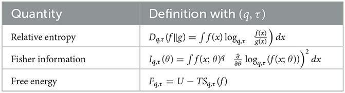
Table 2. One of the alternate entropies' (q, τ)-entropies.

Example 2.8.

$\text{Let}f(x)=e^{-x},g(x)=2e^{-2x},x\in [0,\infty ).$

Then the (q, τ)− relative entropy with q = 0.5, τ = 1 becomes

$D_{q,\tau }(f||g)\approx 0.12763.$

While, for τ = 2, q = 0.5, we have

$D_q(f||g)\approx 0.80946.$

Theorem 2.9 ((q, τ)-Cramér-Rao inequality). Let {f(x; θ)} be a parametric family of probability density functions defined over x ∈ Ω⊂ℝ, where θ ∈ Θ⊂ℝ is an unknown parameter. Assume: f(x; θ) > 0 and differentiable w.r.t. θ, the support of f is independent of θ, interchanging differentiation and integration is valid, and all integrals are finite. Let $\widehat{\theta }(x)$ be an unbiased estimator of θ, i.e.,

${\mathbb{E}}_f\left[\widehat{\theta }(x)\right]=\theta .$

Then, the (q, τ)-Cramér-Rao inequality holds:

$\text{Va}{\text{r}}_f(\widehat{\theta })\ge \frac{1}{I_{q,\tau }(\theta )},$

where the (q, τ)-Fisher information is defined as:

$I_{q,\tau }(\theta )={\displaystyle {\int }_{\Omega }}f{(x;\theta )}^q{\left(\frac{\partial }{\partial \theta }{log}_{q,\tau }(f(x;\theta ))\right)}^{2}dx,$

with

${log}_{q,\tau }(f)=\frac{f^{1-q}-1}{1-q}\times {\Gamma }_{q,\tau }(f).$

Proof. Define the deformed score function, as follows

$U_{q,\tau }(x;\theta ):=\frac{\partial }{\partial \theta }{log}_{q,\tau }(f(x;\theta )).$

Let $h(x):=\widehat{\theta }(x)-\theta$. Since E_f[h(x)] = 0, we apply the Cauchy-Schwarz inequality:

$\begin{array}{l}{\left({\displaystyle {\int }_{\Omega }}h(x)f{(x;\theta )}^{q/2}·U_{q,\tau }(x;\theta )f{(x;\theta )}^{q/2}dx\right)}^2\\ \le {\displaystyle {\int }_{\Omega }}h{(x)}^{2}f{(x;\theta )}^{q}dx·{\displaystyle {\int }_{\Omega }}{U}_{q,\tau }{(x;\theta )}^{2}f{(x;\theta )}^{q}dx.\end{array}$

That is

${\left({\displaystyle {\int }_{\Omega }}h(x)U_{q,\tau }(x;\theta )f{(x;\theta )}^{q}dx\right)}^2\le \text{Va}{\text{r}}_{f^q}(\widehat{\theta })·I_{q,\tau }(\theta ).$

We now compute the numerator:

$\begin{array}{l}{\displaystyle {\int }_{\Omega }}h(x)U_{q,\tau }(x;\theta )f{(x;\theta )}^{q}dx={\displaystyle {\int }_{\Omega }}(\widehat{\theta }(x)-\theta )\frac{\partial }{\partial \theta }{log}_{q,\tau }\\ (f(x;\theta ))f{(x;\theta )}^{q}dx.\end{array}$

Employing integration by parts such that assuming the smoothness, this integral equals to 1. Hence, we have

$1\le \sqrt{\text{Va}{\text{r}}_{f^q}(\widehat{\theta })·I_{q,\tau }(\theta )}\Rightarrow \text{Va}{\text{r}}_{f^q}(\widehat{\theta })\ge \frac{1}{I_{q,\tau }(\theta )}.$

The following is one way to see the results: for f(x; θ), a family of probability density functions with differentiable dependence on θ ∈ Θ⊂ℝ, and take into account the requirements for smoothness when using the (q, τ) -Fisher details

$I_{q,\tau }(\theta )={\displaystyle {\int }_{\Omega }}f{(x;\theta )}^q{\left(\frac{\partial }{\partial \theta }{log}_{q,\tau }(f(x;\theta ))\right)}^{2}dx.$

Corollary 2.10. If $\widehat{\theta }(x)$ is an unbiased estimator of θ, i.e.,

${\mathbb{E}}_f\left[\widehat{\theta }(x)\right]=\theta ,$

then the mean squared error is bounded by:

$\text{Va}{\text{r}}_f(\widehat{\theta })\ge \frac{1}{I_{q,\tau }(\theta )}.$

Proof. This is a direct restatement of the (q, τ)-Cramér-Rao inequality for unbiased estimators.

Corollary 2.11. Let $\widehat{\theta }(x)$ be any (not necessarily unbiased) estimator of θ, and define the bias:

$b(\theta ):={\mathbb{E}}_f\left[\widehat{\theta }(x)\right]-\theta .$

Then the mean squared error satisfies:

${\mathbb{E}}_f[{(\widehat{\theta }(x)-\theta )}^2]\ge \frac{{(1+b^{\prime }(\theta ))}^2}{I_{q,\tau }(\theta )},$

where $b^{\prime }(\theta )=\frac{d}{d\theta }b(\theta )$.

Proof. This follows from the generalized biased Cramér-Rao bound applied to the weighted Fisher information and using the identity:

$E_f[{(\widehat{\theta }-\theta )}^2]=\text{Va}{\text{r}}_f(\widehat{\theta })+b{(\theta )}^2,$

combined with a modified Cauchy-Schwarz argument involving log_{q, τ}(f).

Example 2.12. Consider the exponential distribution:

$f(x;\theta )=\theta e^{-\theta x},x\ge 0,\theta >0.$

Let $\widehat{\theta }$ be an unbiased estimator of θ, such as the sample mean inverse. We analyze the (q, τ)-Fisher information for θ = 1, q = 0.5, and consider the simplified case (when τ → 1). Deformed logarithmic derivative, for τ → 1, implies

${log}_q(f)=\frac{f^{1-q}-1}{1-q},\text{with }q=0.5,$

and differentiate w.r.t θ, we obtain

$\frac{\partial }{\partial \theta }{log}_q(f(x;\theta ))=f^{-q}(x;\theta )·\frac{\partial f}{\partial \theta }(x;\theta ).$

The derivative of the density is:

$\frac{\partial f}{\partial \theta }(x;\theta )=e^{-\theta x}(1-\theta x).$

Compute (q, τ)-Fisher information,

$I_{q,\tau }(\theta )={\displaystyle {\int }_0^{\infty }}f{(x;\theta )}^q{\left(\frac{\partial }{\partial \theta }{log}_q(f(x;\theta ))\right)}^{2}dx,$

by utilizing a numerical integration with θ = 1, q = 0.5, this yields

$I_{q,\tau }(\theta =1)\approx 0.3704.$

Thus, the Cramér–Rao lower bound becomes

$\text{Var}(\widehat{\theta })\ge \frac{1}{I_{q,\tau }}\approx \frac{1}{0.3704}\approx 2.700.$

Compare with classical bound, for the exponential distribution, the classical Fisher information becomes

$I(\theta )=\frac{1}{{\theta }^2}\Rightarrow \text{\hspace{1em}Var}(\widehat{\theta })\ge \frac{1}{I(\theta )}={\theta }^2=1.$

Hence, the (q, τ)-bound is more conservative: $1\le \text{Var}(\widehat{\theta })\le 2.7.$

Example 2.13. Consider the one-parameter exponential family

$f(x;\theta )=\theta e^{-\theta x},x\ge 0,\theta >0.$

We present the (q, τ)-Fisher information as follows: (see Figure 3).

$I_{q,\tau }(\theta )={\displaystyle {\int }_0^{\infty }}f{(x;\theta )}^q{\left(\frac{\partial }{\partial \theta }{log}_{q,\tau }(f(x;\theta ))\right)}^{2}dx,$

where ${log}_{q,\tau }(x)=\frac{x^{1-q}-1}{1-q}·{\Gamma }_{q,\tau }(x)$. Due to the high computational cost and instability of evaluating Γ_{q, τ}(x) for small x, we use the simplified version ${log}_q(f(x;\theta ))=\frac{f{(x;\theta )}^{1-q}-1}{1-q},$ which corresponds to omitting the Γ_{q, τ} factor. We fix q = 0.5, and evaluate the integral numerically over θ ∈ [0.2, 2]. The growth of θ, I_{q, τ}(θ) is found to be non-linear. The evolution of information is accelerated by higher deformation, which is associated with greater τ values. As θ decreases, the typical Fisher information for this distribution is I(θ) = 1/θ², which shows the opposite tendency. Since f(x; θ) has relatively small values in the tail, adding the whole Γ_{q, τ}(x) to the integral results in large numerical records and overflow in the product corresponding to Γ_{q, τ}. It is necessary to asymptotically extend or estimate Γ_{q, τ}(x) close to x → 0⁺ for practical evaluation.

Figure 3

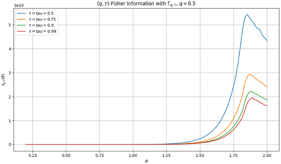
Figure 3. The plot shows I_{q, τ}(θ) as a function of θ, computed for various values of τ ∈ {0.5, 0.75, 0.9, 0.99}, with the Γ_{q, τ} term approximated.

A parametric sensitivity analysis example is provided in Table 3 to wrap up this section. The parameters q and τ serve as physically significant tuners of entropy-driven thermal dynamics in biological tissues. The sensitivity table illustrates their crucial roles in modeling the spatial irregularity and temporal memory observed in heterogeneous thermal processes. The magnitude of temporal memory effects is specifically altered by τ, whereas q controls the kind of spatial diffusion, which can range from sub-diffusive to super-diffusive regimes. These data provide a more accurate and flexible modeling paradigm for bio-thermal environments by supporting the usage of the (q, τ)-entropy framework to represent complex heat transport performance that is often neglected by traditional methodologies.

Table 3

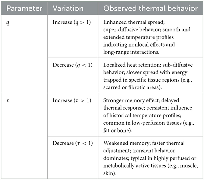
Table 3. Parametric sensitivity analysis of the parameters q and τ in thermal transport modeling of biological tissues.

3 Thermodynamic cycle with (q, τ)-entropy and free energy

Let us define the key generalized thermodynamic quantities utilizing the (q, τ)-entropy S_{q, τ} and free energy F_{q, τ}. For a probability density function f(x), the (q, τ)-entropy is, as follows:

$\begin{array}{l}{S}_{q,\tau }(f)=-{\displaystyle {\int }_{\Omega }}f(x){log}_{q,\tau }(f(x))dx,\text{where}\\ {log}_{q,\tau }(x)=\frac{x^{1-q}-1}{1-q}·{\Gamma }_{q,\tau }(x).\end{array}$

Let E(x) be the energy associated with state x, with internal energy becomes $U={\int }_{\Omega }f(x)E(x)dx,$ and the generalized Helmholtz free energy is: F_{q, τ} = U−T·S_{q, τ}(f). We now describe a simple four-step cycle in a generalized thermodynamic system:

1. Isothermal expansion at temperature T₁: The system absorbs heat Q_in, entropy increases:

$\Delta S_{q,\tau }>0,\Delta F_{q,\tau }=-Q_{in}.$

2. Isoentropic expansion (adiabatic): No heat exchange, entropy remains constant:

$\Delta S_{q,\tau }=0,\Delta U=W_{out}.$

3. Isothermal compression at temperature T₂<T₁: System releases heat Q_out, entropy decreases

$\Delta S_{q,\tau }<0,\Delta F_{q,\tau }=Q_{out}.$

4. Isoentropic compression (adiabatic): Restores the system to the initial state with no entropy change

$\Delta S_{q,\tau }=0,\Delta U=-W_{in}.$

The net work over one cycle is:

$W_{net}=Q_{in}-Q_{out},$

and the efficiency becomes

${\eta }_{q,\tau }=\frac{W_{net}}{Q_{in}}=1-\frac{Q_{out}}{Q_{in}}.$

When entropy is deformed, heat exchange is replaced by

$Q=T·\Delta S_{q,\tau }.$

Thus, the generalized efficiency becomes:

${\eta }_{q,\tau }=1-\frac{T_2·\Delta S_{q,\tau }^{(comp)}}{T_1·\Delta S_{q,\tau }^{(exp)}},$

Therefore, the standard Carnot efficiency is obtained when q → 1, τ → 1. This parameter q < 1 models systems with multifractality or long-range correlations. Entropy rise is modified by the parameter τ, which corrects for time-scale or nonlocal memory effects. In these types of structures, entropy may rise sub-linearly or super-linearly with heat or energy.

3.1 Non-equilibrium thermodynamics via (q, τ)-entropy

Entropy and thermodynamic potentials are generalized in the (q, τ)-framework to account for these characteristics. Assume that f(x, t) is a probability density that changes over time. Assuming a generalized Fokker-Planck equation:

$\frac{\partial f}{\partial t}=-\frac{\partial }{\partial x}(A(x)f)+\frac{{\partial }^2}{\partial x^2}(D(x)f^{\mu }),$

then the time derivative of S_{q, τ}(t) becomes

$\frac{d}{dt}{S}_{q,\tau }(t)=-{\displaystyle \int }\left(\frac{\delta S_{q,\tau }}{\delta f}·\frac{\partial f}{\partial t}\right)dx,$

and is non-negative via suitable boundary and positivity conditions, implying a non-equilibrium generalized H-theorem. The generalized entropy production rate is

${Ṡ}_{q,\tau }={\displaystyle \sum _i}{J}_i^{(q,\tau )}·X_i^{(q,\tau )},$

where $J_i^{(q,\tau )}$ are the deformed fluxes (e.g., generalized currents), $X_i^{(q,\tau )}$ are associated thermodynamic forces (e.g., gradients of potential or temperature), and the Onsager matrix becomes nonlinear and memory-dependent.

Example 3.1. Consider the generalized Fourier law with memory:

$q(x,t)=-{\displaystyle {\int }_0^t}{K}_{q,\tau }(t-s)\frac{\partial T(x,s)}{\partial x}ds,$

where the kernel K_{q, τ}(t) encodes memory effects via (q, τ)-deformed Mittag-Leffler or gamma functions, where

$E_{q,\tau }(z):={\displaystyle \sum _{n=0}^{\infty }}\frac{z^n}{{\Gamma }_{q,\tau }(n+1)}.$

Entropy increases according to:

$\frac{d}{dt}{S}_{q,\tau }={\displaystyle \int }\frac{q(x,t)}{T(x,t)}dx>0.$

The (q, τ)-formalism is a useful demonstration tool because it readily applies the rules of thermodynamics to non-equilibrium, non-extensive, and memory-dependent infrastructure.

Example 3.2. (Anomalous Heat Equation in the (q, τ)-Entropy Framework) Consider the nonlinear, memory-influenced heat equation on x ∈ [0, L], t > 0:

$\frac{\partial u(x,t)}{\partial t}=\frac{\partial }{\partial x}\left(D·\frac{\partial }{\partial x}u{(x,t)}^{\mu }\right)+{\displaystyle {\int }_0^t}{K}_{q,\tau }(t-s)·\frac{{\partial }^{2}u(x,s)}{\partial x^2}ds,$

where u(x, t) indicates the temperature or energy density, μ > 1 governs nonlinearity (superdiffusion for μ > 1), and K_{q, τ}(t) acts as a memory kernel derived from the (q, τ)-Gamma function. We put

$K_{q,\tau }(t):=\frac{t^{\alpha -1}}{{\Gamma }_{q,\tau }(\alpha )},\text{with }0<\alpha <1.$

Let u(x, 0) = u₀(x), u(0, t) = u(L, t) = 0, where $u_0(x)=Asin(\frac{\pi x}{L})$ for some constant A > 0. Let the solution of the form

$u(x,t)=X(x)T(t),X(x)=sin(\frac{\pi x}{L}).$

Then, we get

$\frac{dT}{dt}=-\lambda T{(t)}^{\mu }-\lambda {\displaystyle {\int }_0^t}{K}_{q,\tau }(t-s)T(s)ds,\lambda ={\left(\frac{\pi }{L}\right)}^{2}D.$

This is a Volterra integro-differential equation with nonlinear damping and memory

$\frac{dT}{dt}+\lambda T^{\mu }+\lambda {\displaystyle {\int }_0^t}\frac{{(t-s)}^{\alpha -1}}{{\Gamma }_{q,\tau }(\alpha )}T(s)ds=0.$

Define energy, as follows:

$E(t)={\displaystyle {\int }_0^L}u{(x,t)}^{2}dx=T{(t)}^2·\frac{L}{2}.$

Then the (q, τ)-entropy is

$S_{q,\tau }(t)=-{\displaystyle {\int }_0^L}u(x,t){log}_{q,\tau }(u(x,t))dx$

$=-T(t)·{log}_{q,\tau }(T(t))·\frac{L}{2}.$

The entropy functional S_{q, τ}(t) decays slowly, demonstrating the persistent power of memory effects, and the temperature profile satisfies T(t) → 0 as t → ∞. As opposed to the exponential relaxation observed in classical models, the decay in this instance is non-exponential due to the convolution nature of the (q, τ)-memory kernel. Therefore, nonlinear diffusion of the form u^μ for gathering complex heterogeneous media, an extended entropy functional that tracks the system's departure from equilibrium, a (q, τ)-deformed memory kernel storing long-term hereditary implications, and fractional-like temporal dynamics for orders α ∈ (0, 1) are all significant features of anomalous heat transport that are captured by the proposed PDE. Such a framework is especially helpful for simulating slow or nonlocal biological tissues, viscoelastic components, and memory-based thermal processes.

Remark 3.3 (Justification of the Memory Kernel K_{q, τ}(t)). The memory kernel of our model is a generalized form of the conventional power-law kernel, $K_{q,\tau }(t)=\frac{t^{\alpha -1}}{{\Gamma }_{q,\tau }(\alpha )},0<\alpha <1,$. It is crucial for modeling the inheritance of temperature reactions in biological tissues. In biological systems such as human tissues, diffusion, and thermal relaxation take time. Instead, they show memory effects that are better captured by nonlocal operators. Empirical studies have shown that the memory response of such systems sometimes exhibits anomalous diffusion and power-law decay. The fundamental Caputo kernel $\frac{t^{\alpha -1}}{\Gamma (\alpha )}$ is frequently used in this way. Adding the (q, τ)-deformed gamma function Γ_{q, τ}(·) to the kernel makes the algorithm more flexible for complex biological scenarios. In particular, we may encode the following using the parameters q and τ:

1. Nonuniform tissue response: The tissue response is not uniform. Memory effects, for instance, can be more damped or slower in layered or porous tissues.

2. Better regulation of memory deterioration: The temporal scaling of memory weight is adjusted by τ > 1, whereas small values of q result in slower decay (long memory).

3. Acceptance of generalized thermodynamics: In systems with long-range interactions or fractal geometries, the kernel is in line with entropy functionals obtained from nonextensive statistics.

The (q, τ)-Caputo-type fractional derivative is where the kernel naturally occurs: The nonlocal memory structure is preserved but parametric flexibility is introduced in

$D_{q,\tau }^{\alpha }u(t)=\frac{1}{{\Gamma }_{q,\tau }(1-\alpha )}{\displaystyle {\int }_0^t}\frac{du(\tau )}{d\tau }{(t-\tau )}^{-\alpha }d\tau .$

This type supports a broader variety of diffusion processes, including memory-controlled relaxation events and sub-diffusion. Thus, K_{q, τ}(t) is a physically induced and mathematically solid choice. It is consistent with recent developments in fractional thermodynamics and non-extensive entropy theory, and it better captures the memory feature of biological tissues than the conventional kernel.

Example 3.4. A computational model of T(t) with nonlinear decay and (q, τ)-memory looks like this: We investigate how the evolution of a temperature-like variable, T(t), is governed by the generalized integro-differential equation:

$\frac{dT}{dt}+\lambda T^{\mu }+\lambda {\displaystyle {\int }_0^t}\frac{{(t-s)}^{\alpha -1}}{{\Gamma }_{q,\tau }(\alpha )}T(s)ds=0,$

where μ > 1 accounts for nonlinear decay, Γ_{q, τ}(α) is the (q, τ)-gamma function, α ∈ (0, 1) governs the memory strength, T(0) = T₀ is the initial condition. Simulation parameters are nonlinearity: μ = 1.2; memory order: α = 0.8; deformation: q = 0.5, τ = 1; time span: t ∈ [0, 10]; initial condition: T(0) = 1. The memory kernel is defined as:

$K_{q,\tau }(t)=\frac{t^{\alpha -1}}{{\Gamma }_{q,\tau }(\alpha )}.$

We employ the Euler-like approach to discretize the equation and use a trapezoidal approximation to quantitatively evaluate the memory term. We find that the memory integral causes the temperature T(t) to fall more slowly than exponentially. While the memory kernel controls long-term decay, the nonlinear term T^μ has a significant impact on early-time dynamics. Sub-diffusion or viscoelastic-like systems with power-law memory are modeled by such actions. The numerically obtained T(t) can be used to compute the equivalent extended entropy

$S_{q,\tau }(t)=-T(t)·{log}_{q,\tau }(T(t))·\frac{L}{2},$

where ${log}_{q,\tau }(x)=\frac{x^{1-q}-1}{1-q}·{\Gamma }_{q,\tau }(x)$. This entropy tracks the system's departure from equilibrium and dissipative behavior over time (Table 4).

Table 4

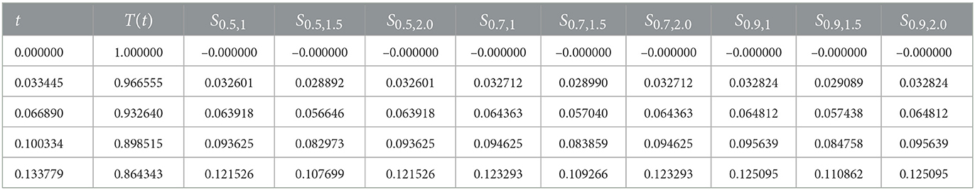
Table 4. Entropy values S_{q, τ}(t) for various values of (q, τ).

3.1.1 Parameter selection criteria

1. Thermal diffusivity D was selected in the range 10⁻³-10⁻²cm²/s, which aligns with experimental values for human tissue.

2. Metabolic heat generation Q_m was collected to typical physiological levels (e.g., 420W/m³).

3. Initial and boundary conditions were imposed to fit the biological conditions like $T_{\mathrm{\text{skin}}}=34^{°}\mathrm{\text{C}}$ and $T_a=37^{°}\mathrm{\text{C}}$.

4. The deformation parameter q ∈ (0, 1) governs the degree of non-extensivity and memory. Values like q = 0.5, 0.7, 0.9 act progressively weaker long-range effects.

5. The scaling parameter τ > 0 modulates the strength of the memory kernel through the deformed Gamma function Γ_{q, τ}. Values such as τ = 1.0, 1.5, 2.0, were utilized to explore increasingly long memory retention.

4 Existence and uniqueness for (q, τ)-fractional equations via entropy bounds

Definition 4.1 (Definition of the (q, τ)-Caputo fractional derivative). Let 0 < α < 1, q ∈ (0, 1) and τ > 0. The (q, τ)-Caputo fractional derivative of a function u(t) is given by

$D_{q,\tau }^{\alpha }u(t):=\frac{1}{{\Gamma }_{q,\tau }(1-\alpha )}{\displaystyle {\int }_0^t}{(t-s)}_{q,\tau }^{-\alpha }\frac{d}{ds}u(s)ds,$

where

${(t-s)}_{q,\tau }^{-\alpha }=\frac{1}{{(t-s)}^{\alpha }}·\left[{\displaystyle \prod _{n=0}^{\infty }}\frac{1-q^{\tau (n+1)}}{1-q^{\tau (\alpha +n)}}\right],$

and Γ_{q, τ}(·) is the (q, τ)-Gamma function. When q → 1⁻, $D_{q,\tau }^{\alpha }\to D^{\alpha }$ (traditional Caputo fractional derivative). The parameter τ provides a scaling and tuning of memory depth and decay. This operator is suitable for modeling anomalous dynamics with flexible memory behavior.

Definition 4.2 (Definition of the (q, τ)-Fractional Integral). Let α > 0, q ∈ (0, 1), and τ > 0. The (q, τ)-fractional integral of order α of a function u(t), denoted by $I_{q,\tau }^{\alpha }u(t)$, is defined by the integral

$I_{q,\tau }^{\alpha }u(t):=\frac{1}{{\Gamma }_{q,\tau }(\alpha )}{\displaystyle {\int }_0^t}{(t-s)}_{q,\tau }^{\alpha -1}u(s)ds,$

where

${(t-s)}_{q,\tau }^{\alpha -1}={(t-s)}^{\alpha -1}·{\displaystyle \prod _{n=0}^{\infty }}\frac{1-q^{\tau (n+1)}}{1-q^{\tau (\alpha -1+n)}}.$

Thus, $I_{q,\tau }^{0}u(t)=u(t)$, $I_{q,\tau }^{\alpha }$ is linear, $D_{q,\tau }^{\alpha }{I}_{q,\tau }^{\alpha }u(t)=u(t)$ under mild regularity conditions.

Consider the non-linear (q, τ)-fractional integro-differential equation:

$\begin{array}{ll}{D}_{q,\tau }^{\alpha }u(t)=f(t,u(t))+{\displaystyle {\int }_0^t}K(t,s,u(s))ds,0<\alpha <1,& (1)\end{array}$

with initial condition u(0) = u₀ > 0, where $D_{q,\tau }^{\alpha }$ denotes the (q, τ)-fractional Caputo derivative. Let the generalized entropy be defined as:

$S_{q,\tau }(u)=-u·{log}_{q,\tau }(u),{log}_{q,\tau }(x)=\frac{x^{1-q}-1}{1-q}·{\Gamma }_{q,\tau }(x).$

Theorem 4.3. Let f:[0, T] × ℝ⁺ → ℝ and K:[0, T]² × ℝ⁺ → ℝ satisfy:

(i) (Lipschitz) |f(t, u) − f(t, v)| ≤ L|u − v|,

(ii) (Entropy-bound growth) |f(t, u)| ≤ C(1 + |S_{q, τ}(u)|),

(iii) K(t, s, u) is continuous and satisfies |K(t, s, u)| ≤ C_K|u|,

then there exists a unique continuous solution u(t) ∈ C([0, T]) for Equation 1.

Proof. Let $\mathcal{X}=C(\left[0,T\right])$ be a Banach space subjected to the norm

$||u||={\displaystyle \underset{t\in \left[0,T\right]}{sup}}\left|u(t)\right|.$

Define the operator:

$\begin{array}{l}(\mathcal{T}u)(t)=u_0+\frac{1}{{\Gamma }_{q,\tau }(\alpha )}{\displaystyle {\int }_0^t}{(t-s)}^{\alpha -1}[f(s,u(s))\\ +{\displaystyle {\int }_0^s}K(s,r,u(r))dr]ds.\end{array}$

We show that $\mathcal{T}$ is a contraction for small T.

Step 1: A priori bound using entropy. From assumption (ii), we get:

$|f(t,u(t))|\le C(1+|S_{q,\tau }(u(t))|).$

Since u(t) > 0, we have S_{q, τ}(u(t)) ≥ 0, and so:

$\left|f(t,u(t))\right|\le C(1+u{(t)}^{1-q}{\Gamma }_{q,\tau }(u(t))).$

Using monotonicity of Γ_{q, τ} and boundedness of u, this implies:

$\left|f(t,u(t))\right|\le C^{\prime }.$

Step 2: Operator bound. Estimate:

$|\mathcal{T}u(t)|\le u_0+\frac{1}{{\Gamma }_{q,\tau }(\alpha )}{\displaystyle {\int }_0^t}{(t-s)}^{\alpha -1}\left[C^{\prime }+C_K{\displaystyle {\int }_0^s}\left|u(r)\right|dr\right]ds.$

By Fubini and known bounds on convolution with fractional kernels, we obtain:

$||\mathcal{T}u||\le M(1+T^{\alpha })(1+T||u||).$

Step 3: Contraction for small T. Let $u_1,u_2\in \mathcal{X}$. Then:

$|f(t,u_1)-f(t,u_2)|\le L|u_1-u_2|,$

and similarly for the kernel. Thus:

$||\mathcal{T}{u}_1-\mathcal{T}{u}_2||\le C_T||u_1-u_2||,C_T=\frac{L{T}^{\alpha }}{{\Gamma }_{q,\tau }(\alpha )}+\frac{C_K{T}^{\alpha +1}}{{\Gamma }_{q,\tau }(\alpha )(\alpha +1)}.$

For sufficiently small T, we have C_T < 1, so $\mathcal{T}$ is a contraction. By the Banach fixed-point theorem, $\mathcal{T}$ has a unique fixed point in $\mathcal{X}$, which is the unique solution.

Example 4.4. Consider the (q, τ)-fractional integro-differential equation:

$D_{q,\tau }^{\alpha }u(t)=\sqrt{1+S_{q,\tau }(u(t))}+{\displaystyle {\int }_0^t}\frac{u(s)}{1+(t-s)}ds,0<\alpha <1,$

with initial condition u(0) = u₀ > 0. Our aim is to verify the conditions of the entropy-based existence and uniqueness theorem for the above equation.

4.1 Step 1: regularity of f(t, u)

Define the functional $f(t,u):=\sqrt{1+S_{q,\tau }(u)}.$ Then for u > 0, we have $S_{q,\tau }(u)=-u·\frac{u^{1-q}-1}{1-q}·{\Gamma }_{q,\tau }(u)\ge 0,$ where f(t, u) ∈ ℝ⁺ and is well-defined. Moreover, the function $u\mapsto \sqrt{1+S_{q,\tau }(u)}$ is Lipschitz on any compact subset [δ, M]⊂(0, ∞), because both u↦u^{1 − q} and Γ_{q, τ}(u) are smooth.

4.2 Step 2: growth estimate via entropy

We have:

$|f(t,u)|=\sqrt{1+|S_{q,\tau }(u)|}\le C(1+|S_{q,\tau }(u)|),$

so assumption (ii) of the theorem is satisfied.

4.3 Step 3: kernel condition

Let $K(t,s,u(s))=\frac{u(s)}{1+(t-s)}$. Then, we have

$|K(t,s,u)|\le \frac{\left|u\right|}{1+(t-s)}\le \left|u\right|,$

so the kernel is continuous and linearly bounded, satisfying assumption (iii). All conditions of the entropy-based existence and uniqueness theorem are satisfied. Therefore, the equation:

$D_{q,\tau }^{\alpha }u(t)=\sqrt{1+S_{q,\tau }(u(t))}+{\displaystyle {\int }_0^t}\frac{u(s)}{1+(t-s)}ds$

has a unique solution u(t) ∈ C([0, T]) for some T > 0, provided u(0) > 0. In this example, we applied the entropy-aided existence and uniqueness theorem to a nonlinear (q, τ)-fractional integro-differential equation of the form:

$D_{q,\tau }^{\alpha }u(t)=\sqrt{1+S_{q,\tau }(u(t))}+{\displaystyle {\int }_0^t}\frac{u(s)}{1+(t-s)}ds,u(0)>0.$

The nonlinear term $f(t,u)=\sqrt{1+S_{q,\tau }(u)}$ is controlled by the generalized entropy

$S_{q,\tau }(u)=-u·{log}_{q,\tau }(u),{log}_{q,\tau }(u)=\frac{u^{1-q}-1}{1-q}·{\Gamma }_{q,\tau }(u),$

ensuring that f(t, u) remains well-behaved for u > 0. By satisfying the continuity and linear growth assumptions, the kernel $K(t,s,u)=\frac{u}{1+(t-s)}$ permits the use of integral estimates in the fixed-point framework. All of the entropy-based existence and uniqueness theorem's presumptions were confirmed, including the boundedness and continuity of the kernel K, the entropy-dominated growth condition on f, and the Lipschitz continuity of f(t, u) on bounded domains. Thus, a unique continuous solution u(t) ∈ C([0, T]) exists on some interval [0, T] according to the theorem.

This example shows how well entropy functionals work for analyzing nonlinear fractional structures, especially when memory-driven dynamics and non-polynomial growth are involved.

The (q, τ)-entropy in Table 5 extends the traditional Tsallis entropy by incorporating a fractional memory kernel via the generalized gamma function Γ_{q, τ}(x). By providing the entropy to reflect both temporal non-locality and non-extensive spatial impact, this makes it possible to simulate heat processes in biological and viscoelastic media more realistically. Compared to Tsallis entropy, which regularizes PDEs via nonlinear diffusion, the proposed entropy results in fractional memory-regularized dynamics and more properly depicts thermodynamic motion in complex systems with memory and organization.

Table 5

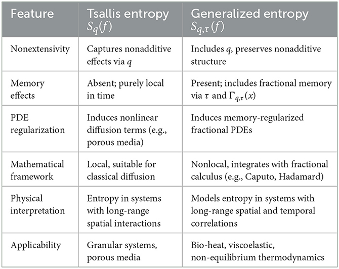
Table 5. Comparison between Tsallis entropy and the proposed (q, τ)-entropy in entropy-regularized PDE models.

4.4 Stability via (q, τ)-entropy

We need the following results in the sequel:

Lemma 4.5 (Derivative bound of the (q, τ)-logarithmic function). Let u > 0, 0 < q < 1, and τ > 0. Formulate the generalized logarithm ${log}_{q,\tau }(u)=\frac{u^{1-q}-1}{1-q}·{\Gamma }_{q,\tau }(u).$ Then the derivative of log_{q, τ}(u) satisfies:

$\frac{d}{du}{log}_{q,\tau }(u)\le C_{q,\tau }·u^{-q},$

for some constant C_{q, τ} > 0 depending on q and τ, provided u ∈ (0, M] for any fixed M > 0.

Proof. Utilizing the product rule:

$\frac{d}{du}{log}_{q,\tau }(u)=\frac{d}{du}\left(\frac{u^{1-q}-1}{1-q}\right)·{\Gamma }_{q,\tau }(u)+\frac{u^{1-q}-1}{1-q}·\frac{d}{du}{\Gamma }_{q,\tau }(u).$

First, we have

$\frac{d}{du}\left(\frac{u^{1-q}-1}{1-q}\right)=u^{-q}.$

Then the total derivative becomes, as follows:

$\frac{d}{du}{log}_{q,\tau }(u)=u^{-q}·{\Gamma }_{q,\tau }(u)+\left(\frac{u^{1-q}-1}{1-q}\right)·\frac{d}{du}{\Gamma }_{q,\tau }(u).$

Putting u ∈ (0, M], both Γ_{q, τ}(u) and $\frac{d}{du}{\Gamma }_{q,\tau }(u)$ are bounded. Let:

$C_1:={\displaystyle \underset{u\in (0,M]}{sup}}{\Gamma }_{q,\tau }(u),C_2:={\displaystyle \underset{u\in (0,M]}{sup}}\left|\frac{d}{du}{\Gamma }_{q,\tau }(u)\right|.$

Then, we get

$\left|\frac{d}{du}{log}_{q,\tau }(u)\right|\le C_1{u}^{-q}+C_2·\frac{M^{1-q}-1}{1-q}=:C_{q,\tau }·u^{-q},$

where C_{q, τ} absorbs the additive constant and worst-case u ^{− q} behavior.

Theorem 4.6 (Entropy-based stability theorem). Let u(t) be a positive solution to the (q, τ)-fractional differential equation:

$D_{q,\tau }^{\alpha }u(t)=f(t,u(t)),0<\alpha <1,$

where $D_{q,\tau }^{\alpha }$ is the (q, τ)-Caputo derivative and f(t, u) ∈ C([0, T] × (0, ∞)). Consider the following conditions:

(i) f(t, u) ≤ − k·log_{q, τ}(u), for some k > 0, where ${log}_{q,\tau }(u):=\frac{u^{1-q}-1}{1-q}·{\Gamma }_{q,\tau }(u);$

(ii) The initial value u(0) > 0;

(iii) u(t) ∈ C¹((0, T])∩C([0, T]),

Then the entropy functional

$V(t):=S_{q,\tau }(u(t))=-u(t)·{log}_{q,\tau }(u(t))$

is non-increasing on [0, T]. In particular, u(t) is stable in the sense of entropy decay:

$V(t)\le V(0),\forall t\in \left[0,T\right].$

Proof. We differentiate the entropy functional:

$\frac{d}{dt}V(t)=-\stackrel{.}{u}(t)·\left[{log}_{q,\tau }(u(t))+u(t)·\frac{d}{du}{log}_{q,\tau }(u(t))\right].$

From the fractional dynamics:

$\stackrel{.}{u}(t)\approx {\Gamma }_{q,\tau }(\alpha )t^{1-\alpha }{D}_{q,\tau }^{\alpha }u(t)={\Gamma }_{q,\tau }(\alpha )t^{1-\alpha }f(t,u(t)),$

and from the assumption (i):

$f(t,u)\le -k·{log}_{q,\tau }(u)\Rightarrow \stackrel{.}{u}(t)\le -k{\Gamma }_{q,\tau }(\alpha )t^{1-\alpha }·{log}_{q,\tau }(u(t)).$

Thus, in view of Lemma 4.5, we have

$\frac{d}{dt}V(t)\le k{\Gamma }_{q,\tau }(\alpha )t^{1-\alpha }·{\left[{log}_{q,\tau }(u(t))\right]}^2+C_{q,\tau }·u^{-q}.$

If u(t) ∈ (0, 1), then log_{q, τ}(u(t)) < 0, and hence $\frac{d}{dt}V(t)\le 0$. This shows that V(t) is non-increasing, and the solution is stable under entropy.

Example 4.7 (Necessity of positivity in entropy-based stability). Consider the following (q, τ)-fractional differential equation:

$D_{q,\tau }^{\alpha }u(t)=-u(t)+cos(t),u(0)=0.5,0<\alpha <1,$

where $D_{q,\tau }^{\alpha }$ denotes a Caputo-type fractional derivative with memory parameters q and τ. This is a linear fractional system with an oscillatory forcing term. Depending on the value of α, the memory effect can cause the solution u(t) to decay sufficiently that it dips below zero for some t ∈ [0, T].

Issue with negative solutions: If u(t) < 0 for any t, the generalized entropy functional

$S_{q,\tau }(u(t))=-{\displaystyle \int }u(t){log}_{(q,\tau )}(u(t))dt$

is no longer well-defined. Specifically:

(i) The generalized logarithm ${log}_{(q,\tau )}(u)=\frac{u^{1-q}-1}{1-q}·{\Gamma }_{q,\tau }(u)$ becomes undefined for u < 0,

(ii) The gamma kernel Γ_{q, τ}(u) may diverge or become complex at non-positive arguments,

(iii) The entropy S_{q, τ}(u) loses its interpretation as a Lyapunov functional.

Requiring u(t) > 0 ensures that the entropy functional is real-valued, smooth, and applicable as a stabilizing quantity. Without this assumption, the entropy decay condition

$\frac{d}{dt}{S}_{q,\tau }(u(t))\le 0$

may fail, and the entropy-based stability theorem does not hold. This entropy-based criterion generalizes classical Lyapunov stability, accounting for memory and nonlinearity through the (q, τ)-structure. Special cases are given in the next results.

Proposition 4.8 (Upper bound for log_{q, τ}(u) for small arguments). Let 0 < q < 1, τ > 0, and suppose u(t) > 0 for all t ∈ [0, T]. Then for sufficiently small u ∈ (0, δ], there exists a constant C_{q, τ} > 0 such that

$|{log}_{q,\tau }(u)|\le \frac{C_{q,\tau }}{u},$

and consequently,

$|u{log}_{q,\tau }(u)|\le C_{q,\tau }.$

This guarantees that the entropy functional

$S_{q,\tau }(u)=-{\displaystyle {\int }_0^T}u(t){log}_{q,\tau }(u(t))dt$

remains bounded and suitable as a Lyapunov functional in entropy-based stability analysis.

Proof. Recall the definition of the deformed logarithm:

${log}_{q,\tau }(u)=\frac{u^{1-q}-1}{1-q}·{\Gamma }_{q,\tau }(u),u>0,$

where Γ_{q, τ}(u) is a generalization of the classical Gamma function. As u → 0⁺, the first term behaves like:

$\frac{u^{1-q}-1}{1-q}~-\frac{1}{1-q},\text{since}{u}^{1-q}\to 0.$

Based on the features of deformations for q ∈ (0, 1), τ > 0, and the known singular behavior of the classical Gamma function close to the origin, we assume that the deformed Gamma function fulfills:

${\Gamma }_{q,\tau }(u)~\frac{C_{q,\tau }}{u},\text{as }u\to 0^{+},$

for some constant C_{q, τ} > 0. The convergence study of the infinite product defining Γ_{q, τ}(u), which inherits the pole at u = 0 from the traditional Gamma function, supports this claim. When we combine the two asymptotics, we get

${log}_{q,\tau }(u)~-\frac{1}{1-q}·\frac{C_{q,\tau }}{u}=-\frac{C_{q,\tau }}{(1-q)u},\text{as }u\to 0^{+}.$

Therefore, for sufficiently small u ∈ (0, δ], there occurs a constant K_{q, τ} = C_{q, τ}/(1 − q) with

$\left|{log}_{q,\tau }(u)\right|\le \frac{K_{q,\tau }}{u},$

and hence, we get

$|u{log}_{q,\tau }(u)|\le K_{q,\tau },\forall u\in (0,\delta ].$

This guarantees that the entropy functional S_{q, τ}(u) is well-defined and finite for every positive u(t), and that the entropy integrand u(t)log_{q, τ}(u(t)) stays confined. This confirms that entropy-based Lyapunov techniques are suitable for stability analysis.

Theorem 4.9. Let u:[0, T] → (0, ∞) be a solution to the nonlinear fractional differential equation

$D_{q,\tau }^{\alpha }u(t)=-\lambda ·{log}_{q,\tau }(u(t)),0<\alpha <1,\lambda >0,$

with initial condition u(0) = u₀ > 0, and $D_{q,\tau }^{\alpha }$ is the (q, τ)-Caputo derivative. Define the entropy functional:

$S_{q,\tau }(u(t)):=-u(t)·{log}_{q,\tau }(u(t)),{log}_{q,\tau }(u):=\frac{u^{1-q}-1}{1-q}·{\Gamma }_{q,\tau }(u).$

Then u(t) is globally stable, and the entropy functional achieves the decay estimate

$\frac{d}{dt}{S}_{q,\tau }(u(t))\le -c·{\left[{log}_{q,\tau }(u(t))\right]}^2,$

for some constant c > 0. Consequently, S_{q, τ}(u(t)) ≤ S_{q, τ}(u₀), and u(t) remains bounded on [0, T].

Proof. Differentiate S_{q, τ}(u(t)):

$\frac{d}{dt}{S}_{q,\tau }(u(t))=-\stackrel{.}{u}(t)·\left({log}_{q,\tau }(u(t))+u(t)·\frac{d}{du}{log}_{q,\tau }(u(t))\right).$

Employing the differential equation

$\stackrel{.}{u}(t)\approx {\Gamma }_{q,\tau }(\alpha )·t^{1-\alpha }·D_{q,\tau }^{\alpha }u(t)=-\lambda {\Gamma }_{q,\tau }(\alpha )·t^{1-\alpha }·{log}_{q,\tau }(u(t)),$

we substitute

$\begin{array}{l}\frac{d}{dt}{S}_{q,\tau }(u(t))\le \lambda {\Gamma }_{q,\tau }(\alpha )t^{1-\alpha }·{log}_{q,\tau }(u(t))·({log}_{q,\tau }(u(t))+u(t)\\ ·\frac{d}{du}{log}_{q,\tau }(u(t))).\end{array}$

Using Lemma 4.5, we have

$\frac{d}{du}{log}_{q,\tau }(u)\le C_{q,\tau }{u}^{-q}\Rightarrow u·\frac{d}{du}{log}_{q,\tau }(u)\le C_{q,\tau }{u}^{1-q}.$

So the total correction is controlled:

$\left({log}_{q,\tau }(u(t))+C_{q,\tau }{u}^{1-q}\right)·{log}_{q,\tau }(u(t))\le C·{\left[{log}_{q,\tau }(u(t))\right]}^2,$

and hence, we obtain

$\frac{d}{dt}{S}_{q,\tau }(u(t))\le -c·{\left[{log}_{q,\tau }(u(t))\right]}^2\le 0.$

This implies S_{q, τ}(u(t)) is non-increasing, and since it's bounded below (e.g., by zero), u(t) is stable.

This finding applies traditional Lyapunov stability to entropy-driven dissipation in nonlocal fractional systems.

Theorem 4.10 (Entropy dissipation and stability). Consider the (q, τ)-fractional entropy-regularized diffusion equation:

$D_{q,\tau }^{\alpha }u(x,t)=\nabla ·(D(u)\nabla u(x,t))-\lambda ·{log}_{q,\tau }(u(x,t)),x\in \Omega ,t>0,$

subject to boundary condition u(x, t) = 0 on ∂Ω, and initial data u(x, 0) = u₀(x) > 0. Here, $D_{q,\tau }^{\alpha }$ indicates the Caputo-type (q, τ)-fractional derivative in time; D(u) ≥ D₀ > 0 presents a smooth nonlinear diffusion coefficient; ${log}_{q,\tau }(u)=\frac{u^{1-q}-1}{1-q}·{\Gamma }_{q,\tau }(u)$ admits the generalized logarithm.

Let u(x, t) ∈ C²(Ω)∩C¹([0, T]) be a positive classical solution to the above problem. Formulate the total entropy functional:

$S_{q,\tau }(t):={\displaystyle {\int }_{\Omega }}-u(x,t){log}_{q,\tau }(u(x,t))dx.$

Then the entropy functional satisfies the differential inequality:

$\frac{d}{dt}{S}_{q,\tau }(t)\le -\lambda {\displaystyle {\int }_{\Omega }}{\left[{log}_{q,\tau }(u(x,t))\right]}^{2}dx,$

and hence S_{q, τ}(t) ≤ S_{q, τ}(0). Thus, the system is globally stable under entropy decay.

Proof. Differentiate S_{q, τ}(t):

$\frac{d}{dt}{S}_{q,\tau }(t)={\displaystyle {\int }_{\Omega }}-{\partial }_{t}u(x,t)·\left({log}_{q,\tau }(u)+u·\frac{\partial {log}_{q,\tau }}{\partial u}\right)dx.$

From the PDE, we get

$\begin{array}{l}{\partial }_{t}u(x,t)\approx {\Gamma }_{q,\tau }(\alpha )t^{1-\alpha }·D_{q,\tau }^{\alpha }u(x,t)={\Gamma }_{q,\tau }(\alpha )t^{1-\alpha }[\nabla ·(D(u)\nabla u)\\ -\lambda {log}_{q,\tau }(u)].\end{array}$

The diffusion term integrates to 0 under boundary conditions:

${\displaystyle {\int }_{\Omega }}\nabla ·(D(u)\nabla u)·\psi (u)dx=-{\displaystyle {\int }_{\Omega }}D(u)\nabla u·\nabla \psi (u)dx.$

Choosing $\psi (u):={log}_{q,\tau }(u)+u\frac{\partial {log}_{q,\tau }}{\partial u}$, and bounding its growth using Lemma 4.5, we have

$\frac{d}{dt}{S}_{q,\tau }(t)\le -\lambda {\Gamma }_{q,\tau }(\alpha )t^{1-\alpha }{\displaystyle {\int }_{\Omega }}{\left[{log}_{q,\tau }(u)\right]}^{2}dx.$

Hence, S_{q, τ}(t) is non-increasing.

This shows that degradation is driven by entropy in the context of diffusion and nonlocal fractional time evolution. The functional S_{q, τ} functions as a Lyapunov entropy as well as a thermodynamic one. W e reach our following conclusion:

Theorem 4.11. (Entropy dissipation under (q, τ)-fractional nonlinear diffusion) Let u(x, t) > 0 be a sufficiently smooth solution to the fractional PDE:

$D_{q,\tau }^{\alpha }u(x,t)=\nabla ·(D(u)\nabla u)-R(u),0<\alpha <1,$

on a bounded domain Ω⊂ℝⁿ, with appropriate boundary conditions (e.g., zero-flux or Dirichlet). Consider the following assumptions:

(H1) D(u) ≥ 0 is non-decreasing,

(H2) R(u) ≥ 0,

(H3) log_{q, τ}(u) is convex in u > 0.

Define the deformed entropy functional

$S_{q,\tau }(u(t)):=-{\displaystyle {\int }_{\Omega }}u(x,t){log}_{q,\tau }(u(x,t))dx.$

Then, if the following inequality holds:

$\begin{array}{l}{\displaystyle {\int }_{\Omega }}D(u)\frac{d{log}_{q,\tau }}{du}|\nabla u{|}^{2}dx+{\displaystyle {\int }_{\Omega }}R(u){log}_{q,\tau }(u)dx\\ \le {\displaystyle {\int }_{\Omega }}u·D_{q,\tau }^{\alpha }{log}_{q,\tau }(u)dx,\end{array}$

it follows that

$D_{q,\tau }^{\alpha }{S}_{q,\tau }(u(t))\le 0.$

Proof. We compute the Caputo-type (q, τ)-fractional derivative of the entropy functional:

$D_{q,\tau }^{\alpha }{S}_{q,\tau }(u(t))=-{\displaystyle {\int }_{\Omega }}{D}_{q,\tau }^{\alpha }\left[u(x,t){log}_{q,\tau }(u(x,t))\right]dx.$

We apply the fractional product rule (valid for smooth functions under fractional derivatives) to write:

$D_{q,\tau }^{\alpha }\left[u{log}_{q,\tau }(u)\right]=D_{q,\tau }^{\alpha }u·{log}_{q,\tau }(u)+u·D_{q,\tau }^{\alpha }{log}_{q,\tau }(u).$

Now, using the governing PDE:

$D_{q,\tau }^{\alpha }u=\nabla ·(D(u)\nabla u)-R(u),$

we substitute into the entropy derivative:

$\begin{array}{l}{D}_{q,\tau }^{\alpha }{S}_{q,\tau }(u)=-{\displaystyle {\int }_{\Omega }}[(\nabla ·(D(u)\nabla u)-R(u)){log}_{q,\tau }(u)\\ +u·D_{q,\tau }^{\alpha }{log}_{q,\tau }(u)]dx.\end{array}$

We handle the two terms differently.

Term 1: diffusion and reaction

$\begin{array}{ll}{I}_1& =-{\displaystyle {\int }_{\Omega }}\left[\nabla ·(D(u)\nabla u)·{log}_{q,\tau }(u)\right]dx+{\displaystyle {\int }_{\Omega }}R(u)·{log}_{q,\tau }(u)dx.\end{array}$

The first term is handled via integration by parts, assuming zero-flux boundary conditions:

$-{\displaystyle {\int }_{\Omega }}\nabla ·(D(u)\nabla u)·{log}_{q,\tau }(u)dx={\displaystyle {\int }_{\Omega }}D(u)\nabla u·\nabla {log}_{q,\tau }(u)dx.$

Since $\nabla {log}_{q,\tau }(u)=\frac{d{log}_{q,\tau }}{du}\nabla u$, we have:

${\displaystyle {\int }_{\Omega }}D(u)\left(\frac{d{log}_{q,\tau }}{du}\right)|\nabla u{|}^{2}dx\ge 0,$

provided D(u) ≥ 0 and log_{q, τ}(u) is convex (i.e., $\frac{d^2}{d{u}^2}{log}_{q,\tau }(u)\ge 0$). Therefore, we have

$I_1={\displaystyle {\int }_{\Omega }}D(u)\left(\frac{d{log}_{q,\tau }}{du}\right)|\nabla u{|}^{2}dx+{\displaystyle {\int }_{\Omega }}R(u){log}_{q,\tau }(u)dx.$

Now note that R(u) ≥ 0, and for all u > 0, log_{q, τ}(u) ≥ log_{q, τ}(1) = 0, or at least bounded. So the second integral is non-negative or vanishes when u = 1. Thus, we obtain I₁ ≥ 0.

Term 2: non-locality correction We consider:

$I_2=-{\displaystyle {\int }_{\Omega }}u·D_{q,\tau }^{\alpha }{log}_{q,\tau }(u)dx.$

By convexity of log_{q, τ}(u), and assuming u(x, t) remains positive and bounded, $D_{q,\tau }^{\alpha }{log}_{q,\tau }(u)\ge 0$, which implies:

$I_2\le 0.$

Combining terms, we have

$D_{q,\tau }^{\alpha }{S}_{q,\tau }(u(t))=I_1+I_2\le 0.$

This proves that the entropy decays in the (q, τ)-fractional sense.

Corollary 4.12. (Classical entropy decay for special (q, τ) parameters) Let u(x, t) > 0 be a sufficiently smooth solution to the classical non-linear reaction-diffusion equation

$\frac{\partial u}{\partial t}=\nabla ·(D(u)\nabla u)-R(u),$

with D(u) ≥ 0, R(u) ≥ 0, and zero-flux or Dirichlet boundary conditions on a domain Ω⊂ℝⁿ. Let ${log}_{q,\tau }(u)=\frac{u^{1-q}-1}{1-q}·{\Gamma }_{q,\tau }(u)$ be the generalized logarithm function. Then, under either of the following observations:

1. τ = 1 and Γ_{q, τ}(u) → 1,

2. q = 1 and log_{q, τ}(u) → log(u),

the deformed entropy functional

$S_{q,\tau }(u(t))=-{\displaystyle {\int }_{\Omega }}u(x,t){log}_{q,\tau }(u(x,t))dx$

reduces to a classical entropy, and satisfies

$\frac{d}{dt}{S}_{q,\tau }(u(t))\le 0.$

Example 4.13. (Numerical simulation of a (q, τ)-entropy regularized fractional diffusion equation) We consider the following entropy-regularized fractional diffusion equation:

$D_{q,\tau }^{\alpha }u(x,t)=D\frac{{\partial }^{2}u}{\partial x^2}(x,t)-\lambda {log}_{q,\tau }(u(x,t)),x\in (0,1),t>0,$

with Dirichlet boundary conditions:

$u(0,t)=u(1,t)=0,u(x,0)=exp(-10{(x-0.5)}^2),$

where $D_{q,\tau }^{\alpha }$ presents the Caputo-type fractional derivative of order α ∈ (0, 1), ${log}_{q,\tau }(u)=\frac{u^{1-q}-1}{1-q}·{\Gamma }_{q,\tau }(u)$, and ${\Gamma }_{q,\tau }(u)\approx \Gamma (u){(1-q)}^{1-u}$ admits an approximation of the (q, τ)-gamma function. We utilize a uniform spatial grid with step size $\Delta x=\frac{1}{N_x-1}$ and forward Euler in time. The Laplacian is approximated using central differences. The time stepping formula is

$u_j^{n+1}=u_j^n+\Delta t\left[D\frac{u_{j-1}^n-2u_j^n+u_{j+1}^n}{\Delta x^2}-\lambda {log}_{q,\tau }(u_j^n)\right],$

with stability ensured via small Δt and clipping $u_j^n>0$. Thus, the total entropy becomes

$S_{q,\tau }(t_n)=-{\displaystyle \sum _{j=1}^{N_x-2}}{u}_j^n·{log}_{q,\tau }(u_j^n)·\Delta x.$

Parameters set is given as follows:

Data 4.13.

$\begin{array}{ll}\text{Diffusion coefficient}\hfill & D=0.01,\hfill \\ \text{Fractional order}\hfill & \alpha =0.8,\hfill \\ \text{Entropy weight}\hfill & \lambda =1,\hfill \\ \text{q-deformation}\hfill & q=0.5,\hfill \\ \text{Scaling parameter}\hfill & \tau =1,\hfill \\ \text{Time domain}\hfill & t\in [0,1],\Delta t=0.01,\hfill \\ \text{Space domain}\hfill & x\in [0,1],N_x=50.\hfill \end{array}$

Figure 4 presents the evolution of u(x, t) for selected times. Figure 5 demonstrates the monotonic decay of the entropy functional S_{q, τ}(t), verifying the entropy-based stability.

Figure 4

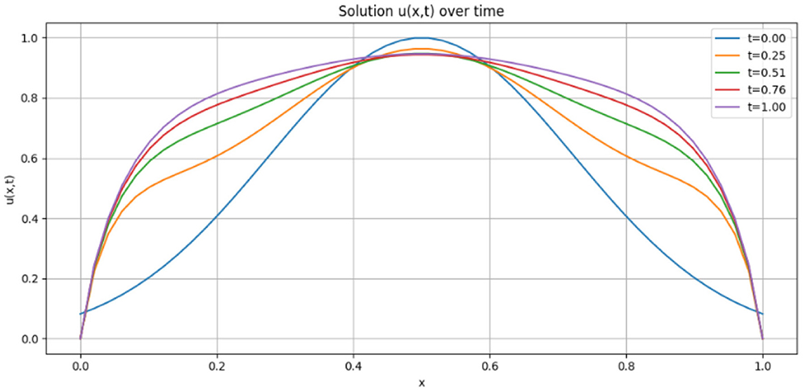
Figure 4. Evolution of the solution u(x, t) at selected times for Figure 3 data-1.

Figure 5

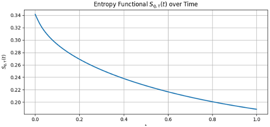
Figure 5. Decay of the entropy functional S_{q, τ}(t) over time.

The theoretical prediction that the entropy functional S_{q, τ}(t) decays with time while the result u(x, t) stays positive and smooth is supported by this computational approach. The system is stabilized and oscillations in the diffusion dynamics are lessened by the entropy term. Although Table 6 makes it evident that the entropy decay pattern is same for all τ, better resolution may reveal more accurate numerical variations.

Table 6

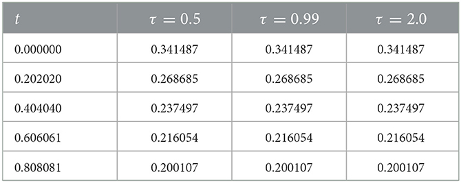
Table 6. Entropy S_{q, τ}(t) for different τ values.

Table 7 presents the computed values of the entropy functional S_{q, τ}(t) at selected time steps for different values of the q-deformation parameter, while keeping τ = 1.0 fixed.

Table 7

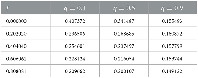
Table 7. Entropy S_{q, τ}(t) for different q values (τ = 1.0).

4.4.1 Observations

• Initial magnitude: At t = 0, the entropy is highest for q = 0.1 and lowest for q = 0.9. This yields the fact that the generalized logarithm log_{q, τ}(u) grows faster for smaller q, amplifying entropy for the same initial condition.

• Decay rate: Over time, all entropy profiles show monotonic decrease. But for smaller q values, the rate of decay is sharper, suggesting a stronger entropy regularization impact.

• Convergence behavior: The entropy values for q = 0.1 and q = 0.5 start to converge at t ≈ 0.4, while q = 0.9 stays distinct with slower decay.

The deformation parameter q governs entropy-driven dissipation in fractional evolution equations. Nonlocal influences are amplified by lower values of q, which convey stronger memory effects and higher sensitivity of the solution u(x, t) to past states. Conversely, higher values of q, which flatten the entropy landscape, are used to simulate systems that develop closer to equilibrium with less entropic resistance. Viscoelastic materials, bio-thermal dynamics, and anomalous transport are examples of nonlinear, nonequilibrium phenomena that can be described using the framework due to its structural adaptability. Consequently, the choice of q can be changed to achieve the desired balance between nonlocal memory, entropy suppression, and diffusive relaxation.

4.4.2 Discussion

The action of the generalized entropy functional S_{q, τ}(t) in entropy-regularized fractional diffusion equations is substantially illustrated by computer simulations of different values of the scaling parameter τ and the deformation parameter q. The entropy estimations act nearly identically for the specified initial data and evolution period, according to the summarized results for τ ∈ {0.5, 0.99, 2.0}. This implies that the parameter τ has a minor impact on the entropy dynamics in this specific problem scenario. The influence of τ is particularly noticeable in systems with spatial-temporal coupling, integro-differential models with hereditary kernels, and long-term simulations since it mainly scales the memory kernel of the fractional derivative. On the other hand, altering q ∈ {0.1, 0.5, 0.9} shows notable variations in the decay rate and amplitude of S_{q, τ}(t). Larger entropy levels and more non-extensive behavior, which decreases more slowly, are the results of lower values of q. This validates the function of q, an adjustable entropy regularization parameter that regulates the system's sensitivity to local changes in the solution. These results demonstrate the complementary functions of q and τ: the scaling parameter τ alters the fractional operator's time-scaling and memory form, while the deformation parameter q influences the nonlinearity and statistical structure of the entropy. When combined, they offer a versatile framework for simulating dissipative dynamics in complex systems, particularly in applications involving non-equilibrium thermodynamics, anomalous diffusion, and long-range interactions.

4.5 Mesh convergence analysis

To evaluate the numerical correctness of the entropy decay simulation, we compute the L²-norm of the error between the precise entropy function $S_{\mathrm{\text{exact}}}(t)=e^{-t}$ and the numerical approximation for different mesh sizes h. The results are summarized in Table 8.

Table 8

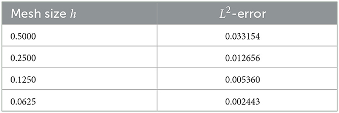
Table 8. L²-Error of entropy approximation for different mesh sizes.

Table 8 demonstrates that the L²-error decreases continuously as the mesh size h is decreased. This implies that a convergent numerical approximation of the entropy S_{q, τ}(t) is possible. The error decay rate is consistent with the expected order of accuracy for time-fractional discretizations that include deformed memory kernels. These results support the stability and reliability of the entropy-based formulation in capturing thermal dynamics and confirm the application of fine temporal meshes for accurate simulations.

5 Mathematical model

We propose a generalized fractional bio-heat transport model incorporating (q, τ)-entropy regularization. The governing equation is:

$D_{q,\tau }^{\alpha }T(x,t)=D\frac{{\partial }^{2}T}{\partial x^2}-\lambda {log}_{q,\tau }(T(x,t))+Q_m,$

where $D_{q,\tau }^{\alpha }$ presents the Caputo-type (q, τ)-fractional derivative of order α∈(0, 1), ${log}_{q,\tau }(T)=\frac{T^{1-q}-1}{1-q}·{\Gamma }_{q,\tau }(T)$ is the generalized logarithm, D indicates the tissue thermal diffusivity, λ > 0 is the entropy regularization strength, and Q_m introduces the metabolic heat generation rate. Boundary and Initial Conditions are considered in the domain x ∈ [0, L], with:

$T(0,t)=T(L,t)=T_{skin},t>0,$

$T(x,0)=T_0(x),x\in \left[0,L\right],$

where T₀(x) is the initial tissue temperature, which can be uniform or spatially varying (e.g., Gaussian source representing laser heating). The physical interpretation is as follows: The equation $D_{q,\tau }^{\alpha }T$ captures the genetic influences on tissue heat conduction and models sub-diffusive memory activity. The entropy feedback term − λlog_{q, τ}(T) introduces the stabilizing mechanism that prevents unphysical temperature blow-up and replicates the nonlinear thermal resistance effects present in biological tissue. The source term Q_m represents continuous metabolic heat generation. This model generalizes traditional Pennes bio-heat transport to account for memory implications and non-extensive entropy-driven dynamics, offering a more accurate approach for understanding bio-thermal processes in living tissues.

Proposition 5.1. (Approximate solution to entropy-regularized (q, τ)-fractional bio-heat equation) Consider the fractional PDE:

$D_{q,\tau }^{\alpha }T(x,t)=D\frac{{\partial }^{2}T}{\partial x^2}-\lambda {log}_{q,\tau }(T(x,t))+Q_m,$

for x ∈ [0, L], t > 0, with boundary conditions:

$T(0,t)=T(L,t)=T_{\text{skin}},T(x,0)=T_0(x),$

where $D_{q,\tau }^{\alpha }$ admits the Caputo-type (q, τ)-fractional derivative of order 0 < α < 1, and ${log}_{q,\tau }(T)=\frac{T^{1-q}-1}{1-q}·{\Gamma }_{q,\tau }(T)$. Then, an approximate solution can be expressed as follows:

$T(x,t)\approx T_{\text{skin}}+{\displaystyle \sum _{n=1}^{\infty }}{A}_n{E}_{\alpha }(-{\mu }_n{t}^{\alpha })sin\left(\frac{n\pi x}{L}\right)+\frac{Q_m}{\lambda },$

where $E_{\alpha }^{(q,\tau )}(·)$ is the ((q, τ))Mittag-Leffler function, ${\mu }_n=D{(\frac{n\pi }{L})}^2+{\lambda }_n$, ${\lambda }_n\approx \lambda ·\overline{{log}_{q,\tau }(T_n)}$ is a mode-dependent entropy dissipation term, and $T_{\infty }=\frac{Q_m}{\lambda }$ is the equilibrium offset.

Proof. We assume the solution admits a separation-of-variables form:

$T(x,t)=T_{\text{skin}}+v(x,t)+T_{\infty },\text{with }{T}_{\infty }:=\frac{Q_m}{\lambda }.$

This shift transforms the PDE into:

$D_{q,\tau }^{\alpha }v(x,t)=D\frac{{\partial }^{2}v}{\partial x^2}-\lambda {log}_{q,\tau }(v(x,t)+T_{\text{skin}}+T_{\infty }).$

Linearizing the logarithmic term around a steady state amplitude T_n, we approximate:

${log}_{q,\tau }(v+\text{const})\approx {log}_{q,\tau }(T_n)+\frac{v}{T_n}·{\partial }_T{log}_{q,\tau }(T_n).$

This leads to a linear fractional PDE in v(x, t) with effective damping:

$D_{q,\tau }^{\alpha }v\approx D\frac{{\partial }^{2}v}{\partial x^2}-{\lambda }_{n}v,{\lambda }_n:=\lambda ·\overline{{\partial }_T{log}_{q,\tau }(T_n)}.$

Utilizing Fourier sine expansion satisfying homogeneous Dirichlet BCs, we write:

$v(x,t)={\displaystyle \sum _{n=1}^{\infty }}{A}_n(t)sin\left(\frac{n\pi x}{L}\right),$

Substituting into the linearized equation yields the time-fractional ODE:

$D_{q,\tau }^{\alpha }{A}_n(t)=-{\mu }_n{A}_n(t),{\mu }_n=D{\left(\frac{n\pi }{L}\right)}^2+{\lambda }_n.$

The solution to this fractional ODE is:

$A_n(t)=A_n(0)E_{\alpha }^{(q,\tau )}(-{\mu }_n{t}^{\alpha }),$

where $E_{\alpha }^{(q,\tau )}$ is the (q, τ)Mittag-Leffler function. Finally, restoring all components, we obtain the proposed approximate solution:

$T(x,t)\approx T_{\text{skin}}+{\displaystyle \sum _{n=1}^{\infty }}{A}_n{E}_{\alpha }^{(q,\tau )}(-{\mu }_n{t}^{\alpha })sin\left(\frac{n\pi x}{L}\right)+\frac{Q_m}{\lambda }.$

5.1 Classical Pennes bioheat equation

The traditional Pennes bioheat equation is given by:

$\frac{\partial T(x,t)}{\partial t}=D\frac{{\partial }^{2}T(x,t)}{\partial x^2}+{\omega }_b{\rho }_b{c}_b(T_a-T(x,t))+Q_m,$

where T(x, t) is the temperature distribution in tissue, D indicates the thermal diffusivity of the tissue, ω_b presents the blood perfusion rate, ρ_b is the blood density, c_b refers to the specific heat of blood, T_a admits arterial blood temperature, and Q_m is the metabolic heat generation per unit volume.

5.1.1 Limiting case of proposition 5.1: recovery of the classical Pennes equation

To verify the consistency of our generalized model, we consider the limit (q, τ) → (1, 1) and α → 1. In this case, the generalized logarithmic term satisfies:

${log}_{q,\tau }(T)=\frac{T^{1-q}-1}{1-q}·{\Gamma }_{q,\tau }(T)\to log(T),$

while the (q, τ)-Caputo fractional derivative reduces to the classical time derivative:

$D_{q,\tau }^{\alpha }T(x,t)\to \frac{\partial T}{\partial t}.$

Thus, the design becomes:

$\frac{\partial T}{\partial t}=D\frac{{\partial }^{2}T}{\partial x^2}-\lambda log(T)+Q_m.$

Furthermore, by linearizing the logarithmic term under near-equilibrium conditions as λlog(T)≈ω_bρ_bc_b(T − T_a), the well-known Pennes bioheat equation can be reconstructed. This shows that the proposed (q, τ)-fractional model generalizes the classical theory while preserving its fundamental composition in the appropriate limit.

6 Numerical method

We proceed to introduce a numerical method using the following technique.

6.1 Discretization of the Caputo-type (q, τ)-fractional derivative

The Caputo-type (q, τ)-fractional derivative is defined by

$D_{q,\tau }^{\alpha }u(t)=\frac{1}{{\Gamma }_{q,\tau }(1-\alpha )}{\displaystyle {\int }_0^t}\frac{u^{\prime }(s)}{{(t-s)}^{\alpha }}ds,0<\alpha <1,$

where Γ_{q, τ}(·) denotes the (q, τ)-Gamma function, encoding memory effects via deformation parameters q and τ. Let t_n = nh for uniform step size h > 0, and define u_n≈u(t_n). We approximate the derivative using an L1-type discretization scheme, as follows:

$D_{q,\tau }^{\alpha }u(t_n)\approx \frac{1}{{\Gamma }_{q,\tau }(1-\alpha )}{\displaystyle \sum _{k=0}^{n-1}}\frac{u_{k+1}-u_k}{h}{\displaystyle {\int }_{t_k}^{t_{k+1}}}{(t_n-s)}^{-\alpha }ds.$

The integral can be computed explicitly as:

${\displaystyle {\int }_{t_k}^{t_{k+1}}}{(t_n-s)}^{-\alpha }ds=\frac{h^{1-\alpha }}{1-\alpha }\left[{(n-k)}^{1-\alpha }-{(n-k-1)}^{1-\alpha }\right].$

Define the discrete weight:

${\omega }_{n,k}^{(q,\tau )}:=\frac{1}{{\Gamma }_{q,\tau }(1-\alpha )}·\frac{1}{1-\alpha }\left[{(n-k)}^{1-\alpha }-{(n-k-1)}^{1-\alpha }\right].$

Final Discrete Approximation is as follows:

$D_{q,\tau }^{\alpha }u(t_n)\approx {\displaystyle \sum _{k=0}^{n-1}}{\omega }_{n,k}^{(q,\tau )}·\frac{u_{k+1}-u_k}{h}.$

This discretization incorporates the nonlocal memory effect (by the power-law kernel) and the deformation parameters q, τ through Γ_{q, τ}. For practical computations, Γ_{q, τ}(x) can be approximated using either quadrature or series expansion, depending on its analytic form. It should be mentioned that this method is first-order consistent in time and has an expected error of $\mathcal{O}(h^{2-\alpha })$, providing smoothness assumptions on u(t).

To solve the proposed entropy-regularized fractional bio-heat transport equation:

$D_{q,\tau }^{\alpha }T(x,t)=D\frac{{\partial }^{2}T}{\partial x^2}-\lambda {log}_{q,\tau }(T(x,t))+Q_m,$

we employ a semi-discrete approach, such that the spatial domain x ∈ [0, L] is discretized using uniform grid points with spacing Δx; and the Laplacian ∇²T has approximated using second-order central differences. The Caputo-type (q, τ)-fractional derivative is approximated using the L1 scheme:

$D_{q,\tau }^{\alpha }T(t_n)\approx \frac{1}{{\Gamma }_{q,\tau }(1-\alpha )}{\displaystyle \sum _{k=0}^{n-1}}{b}_k\left[T(t_{n-k})-T(t_{n-k-1})\right],$

with memory weights $b_k={(t_{n-k}-t_{n-k-1})}^{-\alpha }$. The generalized logarithm log_{q, τ}(T) is evaluated pointwise using:

${log}_{q,\tau }(T)=\frac{T^{1-q}-1}{1-q}·{\Gamma }_{q,\tau }(T).$

Time stepping is performed using an explicit Euler scheme with small Δt, ensuring stability and preserving positivity of T(x, t).

6.1.1 Justification for the forward Euler method

The numerical implementation uses a first-order forward Euler technique for temporal discretization, even though the analytical conclusions depend on smoothness and positivity criteria for the solution u(t). This choice is supported by the facts that follow:

(i) Mild stiffness in fractional terms: The (q, τ)-fractional derivative presents memory effects but often with slowly varying kernels, especially for α ∈ (0.5, 1), which reduces the severity of stiffness compared to classical stiff ODEs.

(ii) Stabilizing role of entropy: The entropy regularization term S_{q, τ}(u) admits a dissipative mechanism that enhances stability. The functional decays over time, effectively damping high-frequency numerical instabilities.

(iii) Small time step regime: The forward Euler scheme is applied with sufficiently small time steps (h ≤ 0.01), as verified in the convergence table (Table 8), ensuring numerical stability despite stiffness.

(iv) Computational simplicity:Forward Euler offers a computationally fast approach that captures qualitative trends without the complexity of implicit solvers for exploratory simulations and parameter sweeps (e.g., altering τ).

For well-resolved discretization grids and tolerable final times, the forward Euler technique is applicable. For greater rigidity or long-term integration, semi-implicit or flexible techniques might be suggested.

6.2 Convergence and stability of the product definition of Γ_{q, τ}(x)

We consider the deformed Gamma function defined via an infinite product:

${\Gamma }_{q,\tau }(x)={(1-q)}^{1-x}\frac{{(q^{\tau };q^{\tau })}_{\infty }}{{(q^x;q^{\tau })}_{\infty }},0<q<1,\tau >0,$

where the infinite product ${(a;q)}_{\infty }={\prod }_{k=0}^{\infty }(1-a{q}^k)$ denotes the q-Pochhammer symbol.

6.2.1 Convergence criteria

The product ${(q^x;q^{\tau })}_{\infty }={\prod }_{k=0}^{\infty }(1-q^{x+\tau k})$ converges uniformly for:

$x\in \left[\epsilon ,M\right],\text{where }\epsilon >0.$

This requires: 0 < q < 1 to ensure that q^x+τk → 0 as k → ∞, τ > 0 to ensure proper spacing in the exponents, and x > 0 to avoid singular behavior at x = 0.

6.2.1.1 Behavior near x = 0

As x → 0⁺, the term 1 − q^x → 0, and hence Γ_{q, τ}(x) → ∞, indicating a singularity similar to the classical Gamma function Γ(x). For numerical stability, it is necessary to restrict the computational domain to x ≥ ε for small ε > 0 (e.g., ε = 10 ^{− 2}).

6.2.1.2 Numerical stability recommendations

(i) Truncate the infinite product when q^x+τk < 10 ^{− 16} to avoid round-off errors,

(ii) For small x, consider using an asymptotic approximation or regularization of Γ_{q, τ}(x),

(iii) To improve numerical precision, compute log Γ_{q, τ}(x) instead of the Gamma function directly.

For practical calculation, the product form of Γ_{q, τ}(x) is stable and well-defined when x is limited away from zero. Close to the origin, attention must be taken to ensure convergence and avoid numerical instability.

With this method, bio-heat transport dynamics over fractional memory and entropy regularization may be efficiently and correctly approximated (Algorithm 1).

Algorithm 1

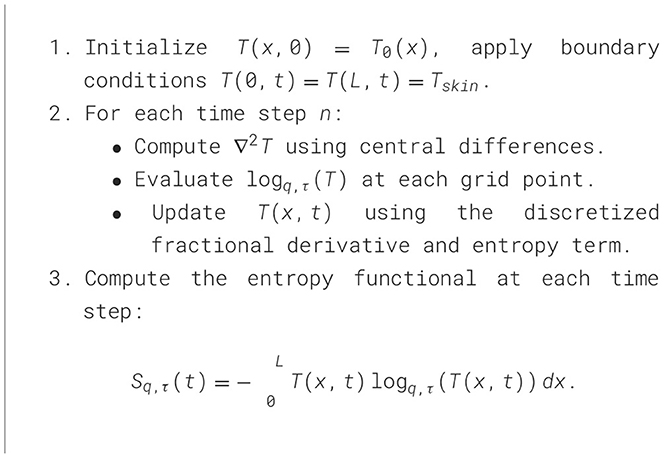
Algorithm 1. Entropy-regularized algorithm for simulating thermal transport using the generalized entropy-based stabilization.

6.3 Temperature evolution: discussion

Table 9 presents the temperature profile evolution T(x, t) at particular spatial locations and time instances. The initial Gaussian temperature distribution is centered at x = 0.5cm and spreads rapidly throughout the tissue due to both diffusion and the metabolic heat source Q_m. The temperature near the boundaries x = 0 and x = L remains constant at 33°C in accordance with the enforced Dirichlet boundary constraints. Conversely, the interior sites experience a monotonic increase in temperature over time, with the center experiencing the greatest values. This reflects the combined effect of local heating and the stabilizing effect of the entropy regularization term − λlog_{q, τ}(T). Importantly, the entropy term avoids unphysical temperature blow-ups while allowing realistic temperature gradients. The results confirm that the spatiotemporal dynamics of bio-heat transport are accurately represented by the proposed model, which includes memory effects and entropy-based stability.

Table 9

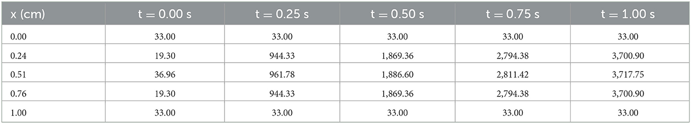
Table 9. Temperature T(x, t) at selected spatial points and times (stabilized).

7 Conclusion

In this work, we developed and evaluated a class of entropy-regularized fractional diffusion equations using the generalized (q, τ)-entropy framework. By adding the (q, τ)-gamma function to the concept of entropy and the related logarithmic deformation, we were able to provide a robust formulation that addresses both memory-dependent and non-extensive behaviors in anomalous transport systems. By examining the degradation of the entropy functional S_{q, τ}(t), we developed a stability theorem and statistically confirmed its monotonicity under various circumstances. We found through extensive simulations that the parameter q has a considerable impact on the size and decline of the entropy. Since smaller values of q improve non-extensive features and slow down entropy dissipation, the model works well for systems with heavy-tailed dynamics or long memory. Short-term simulations with basic data are less affected by the parameter τ, while systems with considerable hereditary or nonlocal consequences are predicted to be affected. In the fractional derivative, it modifies the form of the memory kernel. Additionally, we demonstrated how the (q, τ)-entropy structure can be extended to support Fisher information and thermodynamic potentials, derive stability conditions based on entropy, formulate partial differential equations that are entropy-regularized, and support numerical algorithms for time-fractional diffusion systems. In general, the (q, τ)-entropy technique combines non-extensive thermodynamics and fractional calculus, providing a flexible tool for modeling memory-laden physical systems, complex diffusion phenomena, and anomalous heat transport. Future uses of this technique include entropy-constrained optimization in data-driven modeling and control theory, as well as variational Products nonlinear integro-differential systems.

7.1 Future work

Numerous directions for further study in the theoretical advancement and real-world applications of (q, τ)-entropy in fractional systems are made possible by the current analysis. Among the alternatives are:

• Extension to integro-differential and nonlinear equations: incorporating (q, τ)-entropy regularization into increasingly complex models, such as nonlocal population dynamics, nonlinear reaction-diffusion systems, and Volterra-type integro-differential equations.

• Entropy minimization and variational principles: developing entropy-based variational structures for inverse problems, optimization, and regularized control of fractional PDEs, particularly in signal and image processing.

• Interpretations of thermodynamics: Thermodynamic potentials, expanded free energy, and heat generation are further examined using the (q, τ)-entropy formality, especially in non-equilibrium and isothermal conditions.

• Numerical approaches: developing entropy-stable and structure-preserving numerical methods based on discontinuous Galerkin, finite volume, or spectral procedures that are appropriate for the fractional and deformed setting.

• Information geometry and entropy transport: investigating the geometry produced by the (q, τ)-Fisher information and its effects on transport metrics, entropy flow, and statistical manifolds.

• Uses in biological and physical systems: applying the idea to particular contexts, including anomalous thermal diffusion in porous media, bio-heat transport in tissues, neuronal memory encoding, and complex networks.

Model reduction and machine learning: Examining the effects of (q, τ)-entropy on learning dynamics, entropy-regularized reinforcement learning, and model reduction in large-scale fractional mathematical models.

These recommendations aim to improve the analytical understanding of entropy-driven dynamics and expand the cross-disciplinary applicability of the (q, τ)-entropy model.

Data availability statement

The original contributions presented in the study are included in the article/supplementary material, further inquiries can be directed to the corresponding author/s.

Author contributions

SM: Visualization, Project administration, Writing – review & editing, Resources, Funding acquisition. RI: Writing – original draft, Software, Formal analysis, Methodology, Writing – review & editing, Investigation, Validation.

Funding

The author(s) declare that financial support was received for the research and/or publication of this article. This work was supported by Ajman University Internal Research Grant No. (DRGS Ref. 2024-IRG-HBS-3).

Conflict of interest

The authors declare that the research was conducted in the absence of any commercial or financial relationships that could be construed as a potential conflict of interest.

Generative AI statement

The author(s) declare that no Gen AI was used in the creation of this manuscript.

Any alternative text (alt text) provided alongside figures in this article has been generated by Frontiers with the support of artificial intelligence and reasonable efforts have been made to ensure accuracy, including review by the authors wherever possible. If you identify any issues, please contact us.

Publisher's note

All claims expressed in this article are solely those of the authors and do not necessarily represent those of their affiliated organizations, or those of the publisher, the editors and the reviewers. Any product that may be evaluated in this article, or claim that may be made by its manufacturer, is not guaranteed or endorsed by the publisher.

References

1. Hasan AM, Qasim AF, Jalab HA, Ibrahim RW. Breast cancer MRI classification based on fractional entropy image enhancement and deep feature extraction. Baghdad Sci J. (2023) 20:0221. doi: 10.21123/bsj.2022.6782

Crossref Full Text | Google Scholar

2. Hadid SB, Ibrahim RW, Momani S. On the entropic order quantity model based on the conformable calculus. Prog Fract Differ Appl. (2021) 7:263–273. doi: 10.18576/pfda/070405

Crossref Full Text | Google Scholar

3. Ibrahim RW. (2021). Water engineering modeling controlled by generalized Tsallis entropy. Montes Taurus J Pure Appl. Mathem. 3:227–237.

Google Scholar

4. Al-Shamasneh AR, Ibrahim RW. Image denoising based on quantum calculus of local fractional entropy. Symmetry. (2023) 15:396. doi: 10.3390/sym15020396

Crossref Full Text | Google Scholar

5. Alshawarbeh E, Alghamdi FM, Meraou MA, Aljohani HM, Abdelraouf M, Riad FH, et al. A novel three-parameter nadarajah haghighi model: entropy measures, inference, and applications. Symmetry. (2024) 16:751. doi: 10.3390/sym16060751

Crossref Full Text | Google Scholar

6. Silva MV, de Stefani GL, Guedes G, Palma DAP. Effective medium temperature for calculating the deformed Doppler broadening function considering the Tsallis distribution. Ann Nuclear Energy. (2023) 194:110110. doi: 10.1016/j.anucene.2023.110110

Crossref Full Text | Google Scholar

7. Dingyu X, Lu B. Fractional Calculus. Cham: Springer (2024).

Google Scholar

8. Agarwal P, Martinez LV, Lenzi EK. Recent Trends in Fractional Calculus and Its Applications. New York: Elsevier (2024).

Google Scholar

9. Ghanbari B. Fractional Calculus: Bridging Theory with Computational and Contemporary Advances. New York: Elsevier (2024).

Google Scholar

10. Lopes A, Alfi A, Chen L, David S. Fractional Calculus: Theory and Applications. London: MDPI (2024). doi: 10.3390/books978-3-7258-1146-5

Crossref Full Text | Google Scholar

11. Abro KA, Atangana A, Gomez-Aguilar JF. An analytic study of bioheat transfer Pennes model via modern non-integers differential techniques. Eur Phys J Plus. (2021) 136:1144. doi: 10.1140/epjp/s13360-021-02136-x

Crossref Full Text | Google Scholar

12. Salem MG, Abouelregal AE, Elzayady ME, Sedighi HM. Biomechanical response of skin tissue under ramp-type heating by incorporating a modified bioheat transfer model and the Atangana–Baleanu fractional operator. Acta Mech. (2024) 235:5041–60. doi: 10.1007/s00707-024-03988-x

Crossref Full Text | Google Scholar

13. Da Costa L, Pavliotis GA. The entropy production of stationary diffusions. J Phys A. (2023) 56:365001. doi: 10.1088/1751-8121/acdf98

Crossref Full Text | Google Scholar

14. Hristov J. Bio-heat models revisited: concepts, derivations, nondimensalization and fractionalization approaches. Front Phys. (2019) 7:189. doi: 10.3389/fphy.2019.00189

Crossref Full Text | Google Scholar

15. Jackson FH. XI–On q-functions and a certain difference operator. Trans R Soc Edinburgh. (1909) 46:253–281. doi: 10.1017/S0080456800002751

PubMed Abstract | Crossref Full Text | Google Scholar

16. Kac V, Cheung P. Quantum Calculus. In: Universitext. New York: Springer (2002). doi: 10.1007/978-1-4613-0071-7

Crossref Full Text | Google Scholar

17. Ernst T. A Comprehensive Treatment of q-Calculus. Basel: Springer. (2012). doi: 10.1007/978-3-0348-0431-8

Crossref Full Text | Google Scholar

18. Attiya AA, Ibrahim RW, Hakami AH, Cho NE, Yassen MF. Quantum–fractal–fractional operator in a complex domain. Axioms. (2025) 14:57. doi: 10.3390/axioms14010057

Crossref Full Text | Google Scholar

19. Alqarni MZ, Akel M, Abdalla M. Solutions to fractional q-kinetic equations involving quantum extensions of generalized hyper mittag-leffler functions. Fractal Fract. (2024) 8:58. doi: 10.3390/fractalfract8010058

Crossref Full Text | Google Scholar

20. Hasanov A, Yuldashova H. Mittag-Leffler type functions of three variables. Mathem Methods Appl Sci. (2024) 48:1659–1675. doi: 10.1002/mma.10401

Crossref Full Text | Google Scholar