Inverse problems in covariate data analysis

The fact that Pearson's correlation coefficient and effect size are perspective functions of covariance parameters demonstrates that how covariance is defined is one of the most important issues in data analysis. We suggest that covariance analysis for pairwise numeric, categorical, and mixed numeric-categorical data types are mathematically distinct problems. This is because of the disparate algebraic properties and systematic effects associated with numeric and categorical quantities. We examine the weighted least squares (WLS) formulation of linear regression and obtain definitions for heteroscedastic covariance and variance. Covariance and variance as functions of centered variable vectors are instrumental quantities. Then it is essential that the instrumental effects cancel when dividing covariance by the variance to estimate the slope in linear regression. The tensor product form of the covariance demonstrates that the composite properties of variable vectors are intrinsic to covariate data analysis. The solution of the inverse problem for linear regression takes the form of a relation between slope and covariance parameters, and requires the specification of an error model for the data; otherwise, the inverse problem is ill-posed. We propose that, in current practice, the term “effect size” is ambiguous because it does not distinguish between the different algebraic components of the inverse problem in a case-control data analysis. Then, it is necessary to identify the analogs of WLS covariance for case-control data and to distinguish between covariance and functional parameters in effect size analysis. The development of effect size methodology for studies of complex systems is complicated by the fact that the functional inverse problem is ill-posed.

1 Introduction

In applied mathematics, the computational challenge of converting data into information is termed the “inverse problem” [1, 2]. Forward operators specify the mapping of a system's functional coordinates onto its observable properties. Then, mapping data to functional parameters involves the inversion of forward operators. The correlation concept is widely used in data analysis with formulations for Pearson's r, the point-biserial coefficient (rpb), and ϕ [3]. The latter are categorical variants of r where one or both of the covariates in rpb and ϕ, respectively, are associated with binary outcomes. However, both rpb as an effect size measure [4] and ϕ² as a linkage disequilibrium (LD) measure [5] are confounded by unbalanced sample sizes; in LD analysis, ϕ² is referred to as r². Moreover, there are still fundamental questions about the treatment of measurement error in linear regression [6] and the associated attenuation of Pearson's r [7], and the meaning of effect size [8]. Our research is motivated by high-dimensional data analysis problems in the application of genome-wide association studies (GWAS) [9] and RNA-Seq gene expression [10] technologies for agricultural R&D. This involves using statistical association methods to search large biological datasets [11, 12] to identify markers for improving the agronomic performance of crop species. However, high-dimensional data analysis is challenging because deducing functional models for a complex system from data is an ill-posed inverse problem [13]. Then, the lack of consensus on the merits of effect size [14, 15] stems from the inability to connect covariance parameters with the functional or model-dependent part of the inverse problem. In recent work, we discussed underlying algebraic issues in the formulations for ϕ, rpb, and r. The factorization and identification of the four alternative forms of marginal scaling invariant proportions (MP) for a 2 × 2 contingency table and the correspondence between Gini information gain and the ϕ coefficient in classification and regression tree (CART) methodology are described in [16]. We also demonstrated that using the difference between MPs as an effect size measure in CART yields more intuitive results than ϕ. CART [17, 18] is an important machine learning technique for exploring covariance effects in multivariate data, especially for problems where the development of functional models is difficult [19, 20]. The covariate sort algorithm for identifying the statistical parameters for point-biserial data (v_pb) and the correspondence between mean squared error information gain and rpb in CART are described in Luck [21]. We also demonstrated that the non-overlap proportion (ρ_pb) and Cohen's d offer more intuitive results in CART compared to rpb. In Luck [22], we describe the parametric linear regression (PLR) algorithm for fitting a straight line in m-dimensions, along with the formulations of multiway parametric covariance vectors and correlation coefficients. The term “parametric” comes from the fact that the linear relation is parameterized by a weighted average for the linearly related variable vectors (LRVVs). Our investigation of the PLR problem is motivated by the normalization problem in RNA-Seq data analysis [23]. Scaling corrections are needed to adjust for systematic error arising from instrumental variation in read counts between samples. The read count values for a sample can range over more than three orders of magnitude with heteroscedastic signal-to-noise ratios [22]. Then, PLR analysis is important in estimating parameters for the best fit m-dimensional line for an RNA-Seq dataset, which can then be transformed to adjust for the systematic error across a set of samples.

Covariance serves as the elementary measure of bivariate dependence in r. Consequently, we take the view that covariance is a fundamental concept, while the correlation coefficient and effect size correspond to perspective functions of covariance parameters. Covariance alone does not imply causation. Our objective is to describe how the covariance concept is used in solving inverse problems for the three covariate data types and demonstrate that the usual textbook definitions for sample [24] and random variable [25] covariance coefficients are not sufficient for practical applications. The main novel contributions of this work are centered on two aspects of covariate data analysis, as follows:

(1) Weighted least squares (WLS) methods are important in accounting for data quality and experimental error in solving inverse problems for real-world data analysis. To the best of our knowledge, there are no previous reports [26, 27] on the formulation of the WLS or heteroscedastic covariance coefficient for linear regression. We use the terms “WLS” and “heteroscedastic” synonymously in referring to covariance and variance coefficients. The Cheng and Riu paper [6] discusses the importance of replicated measurements for assessing experimental errors and the treatment of heteroscedasticity in linear measurement error regression (MER). We show that the parametric representation is necessary for the partitioning of residual effects and the formulation of heteroscedastic covariance for MER. Thus, the emphasis in Luck [22] on the role of the Moore-Penrose inverse algorithm in MER for treating heteroscedastic effects, while covariance is homoscedastic, is not warranted. The estimate for the PLR slope is obtained by dividing the WLS covariance by the corresponding WLS variance (Equations 20, 26), where the weights account for the errors in the data for the dependent variable. This formulation demonstrates that it is necessary to adjust for measurement error within the covariance itself, which contrasts with the use of the reliability ratio as a correction factor for the attenuation of the slope due to measurement error [28]. Equations 20, 26 demonstrate that the solution for the inverse problem (SIP) for PLR is expressed as a relation between functional and covariance parameters. Furthermore, the spacings between data points in an MER graph are determined by the experimental procedure, which implies that covariance, variance, and the correlation coefficient as functions of centered variable vectors (VVs) are instrumental quantities. The heteroscedastic PLR correlation coefficient (rPLRw) is defined as the WLS contraction of multiway Pearson correlation and LRVV alignment tensors (Equation 30). In Section 3, we use Monte Carlo (MC) simulations of heteroscedastic covariance for LRVV data with varying dynamic range (DR) to demonstrate the instrumental nature of covariance and correlation.

(2) We describe an algebraic scheme (Equation 31) that specifies the main components of the inverse problem in case-control data analysis. Then, in current practice, the term ‘effect size' actually refers to a compound algebraic problem, which leads to ambiguity in the debate about the merits of effect size. By analogy with the SIP for PLR, we suggest that it's important to separate the two main components: case-control covariance and functional parameters for the system response. Then, it is necessary to identify the case-control parameters for categorical (Section 2.3.2) and point-biserial data (Section 2.3.3). Covariance is associated with the center of mass coordinates (Equation 33) for the case-control parameters, and effect size requires the specification of the relation between the covariance and functional parameters for the case-control response. Our framework shows that accounting for instrumental effects requires distinct formulations for covariance and correlation for the three pairwise data types: numeric (ℝ × ℝ), categorical ($\mathcal{C}$₂ × $\mathcal{C}$₂), and point-biserial ($\mathcal{C}$₂ × ℝ) (Proposition 3). This finding contrasts with current practice, where Pearson's r formula is regarded as providing the general framework for the formulation of correlation for all three covariate data types but requires the artificial {0|1}-numeric substitution procedure for dichotomous data [29, 30].

2 Methods

In this section, we discuss the fact that covariance, as a measure of bivariate dependence, is an essential component in the SIP for covariate data analysis. There is a different covariance problem associated with each of the three distinct covariate data types. For numeric data, Equation 20 demonstrates that the SIP takes the form of a relation between model parameters and WLS covariance for PLR. We provide a comprehensive discussion of the instrumental heteroscedastic properties of covariance (Equation 26) and correlation (Equation 30). We use the term “case-control” generically to refer to classifications obtained through an instrumental process. In the usual experimental protocol, the classifications result from observing the system's behavior under contrasting “case” and “control” conditions. For example, the CART algorithm involves an exhaustive search over binary partitions of multivariate data to create a decision tree [16, 21]. Similarly, in GWAS, the SNPs are instrumental in partitioning the phenotype or trait data in the search for causal effects [31]. In case-control data analysis, the term ‘effect size' refers to statistical measures of system response [8]. However, in current practice, the effect size is ambiguous because it does not distinguish between the different algebraic factors in the inverse problem (Equation 31). By analogy with Equation 20, we propose that specifying the SIP is necessary in defining effect size; then it's important to distinguish between case-control covariance and functional parameters. From now on, the term “effect size” refers to the functional form, unless otherwise stated. Then, it is necessary to identify bivariate parameters that serve as the analogs of WLS covariance in case-control data analysis.

2.1 Notation

Detailed discussions of our notation and terminology for covariate data analysis are found in Luck [16, 21, 22]. By necessity, those papers serve as the primary source for definitions and explanations of important concepts such as parametric covariance vector, m-way correlation, non-overlap proportion, and MP. Those concepts cannot be adequately explained by a few short definitions. Comprehensive discussions of linear algebra and vector spaces are found in many data analysis textbooks [32–34]. Scalars are denoted by lowercase italics, a, vectors by bold lowercase letters, y ≡ (y_i) ≡ (y₁, y₂, y₃, …, y_dim(y)), and matrices by bold uppercase letters, X ≡ [x_ij]. Suppose the functional principles that determine the behavior or state of a system are expressed in terms of the parameter vector, h ∈ ℝ^h. Then, the observed values of a property, Y, are given by the forward equation [2],

$\begin{array}{ll}{y}_i={\mathcal{M}}_Y({\text{h}}_i)+e_{y_i},& (1)\end{array}$

where $\mathcal{M}$_Y(h_i) is the forward operator and e_yi is the residual error. The Y subscript indicates that $\mathcal{M}$_Y is specified for each element of the set of observable quantities, Y ∈ $\mathcal{O}$. Then, an instrumental process ($\mathcal{I}$) makes n joint observations for m experimental quantities to produce a dataset, {y_ij|y_ij ∈ G, 1 ≤ i ≤ n, 1 ≤ j ≤ m}, where the generic data type can be either numeric or categorical, G = ℝ|$\mathcal{C}$. We use convenient terminology from the statistics literature where each axis of a regression graph is assigned to a VV, ${\text{y}}_j\in {ℝ}^n$, the linear combinations $\sum _j{k}_j{\text{y}}_j$ are elements of the variable space, and each point in the graph corresponds to an observation vector ${\text{y}}_{(i)}\in {ℝ}^m$ [24]. A didactic discussion of VVs and the fact that various formulae for covariance, correlation, and linear regression can be given geometric interpretations is found in Rodgers and Nicewander [3]. However, we observe that the variable space framework implies that the data must be regarded as corresponding to the Cartesian product,

$\begin{array}{ll}Y=({\text{y}}_j),& (2)\end{array}$

where ${\text{y}}_j\in {𝔾}^n$, and dim($\mathcal{Y}$) = n × m. Then, the inverse problem in covariate data analysis is summarized in the following scheme:

$\begin{array}{ll}(h_i)\stackrel{ℐ}{\mapsto }\mathcal{Y}\stackrel{\mathcal{A}}{\mapsto }v\stackrel{\left\{{ℳ}_{Y_j}^{-1}\right\}}{\mapsto }E(h),& (3)\end{array}$

where $\mathcal{I}$ creates a data set, $\mathcal{Y}$, for instantiations of a system with functional coordinates (h_i), an algorithm ($\mathcal{A}$) produces the statistical parameters, v, and the set of inverse operators $\left\{{\mathcal{M}}_{Y_j}^{-1}\right\}$ for the observable quantities, {Y_j}, produces estimates for the functional parameters (E(h)). This work is particularly concerned with the application of the covariance concept in solving inverse problems for covariate data. This approach contrasts with the statistics literature, where sample covariance [3] and random variable covariance [25] serve only as abstract forms because they are defined without reference to an inverse problem. The fact that categorical data do not form vector spaces implies that there are distinct covariance analysis problems associated with the three different pairwise data types: linear regression for (ℝ × ℝ), point-biserial for ($\mathcal{C}$₂ × ℝ), and categorical for ($\mathcal{C}$₂ × $\mathcal{C}$₂). The subscript for $\mathcal{C}$₂ indicates the number of categories, and the bi-categorical restriction is imposed because there are no standard procedures for constructing center of mass coordinates for systems with more than two degrees of freedom (Section 2.3 of [21]). We use the term “point-biserial” generically to refer to the mixed $\mathcal{C}$₂ × ℝ data type because of the connection with rpb [30], emphasizing the fact that we are interested in the composite properties of (c, y) data. We use the term “covariate data” when referring to generic quantities of the form ${\text{y}}_j\in G^n$ and regard the algebra of variable vectors ${\text{y}}_j\in {ℝ}^n$ as a special case. Our objective is to discuss the fact that:

For numeric data, WLS covariance is associated with inner and tensor products for centered LRVVs (Equation 18). For categorical data, covariance is associated with MP for a 2 × 2 contingency table [16]. For point-biserial data, covariance is associated with the Cartesian product of statistical parameters from the covariate sort algorithm using the grouping property of categorical data and the ordering property of numerical data [21].

2.2 WLS parametric covariance for linearly related variable vectors

The standard formulation of covariance in linear regression is limited to two dimensions because it is based on the Cartesian representation, y = f(x). In Luck [22], the parametric representation provides the necessary algebraic framework for solving the general multidimensional linear regression problem. However, that work treats covariance as homoscedastic and overemphasizes the importance of the Moore-Penrose inverse when estimating the WLS model parameters. In this section, the objective is to describe the use of the WLS parametric covariance vector in partitioning heteroscedastic residual effects for LRVVs. We briefly introduce various statistical quantities (Equations 4–7) from the PLR paper [22], then we derive the heteroscedastic formulations for WLS covariance (Proposition 1) and the PLR correlation coefficient (Equation 30). In Section 3, we use MC simulations to illustrate the difference between the correlation coefficients for homoscedastic (Equation 35 in Luck [22]) and heteroscedastic covariance (Equation 30).

Consider a set of LRVVs $\left\{Y=({\text{y}}_j)|{\text{y}}_j\in {ℝ}^n\right\}$ with a corresponding convex set [35] of weighted averages τ ∈ conv($\mathcal{Y}$),

$\begin{array}{ll}\begin{array}{ll}\tau \hfill & =\frac{{\displaystyle {\sum }_j{w}_j}{y}_j}{{\displaystyle {\sum }_j{w}_j}},\hfill \end{array}& (4)\end{array}$

with 0 ≤ w_j. The residual error for the difference between the observed and true $({\text{y}}_j^{*})$ values is denoted ${\text{e}}_j={\text{y}}_j-{\text{y}}_j^{*}$; the ‘*' symbol indicates true or fixed values. We regard the errors {e_ij} as associated with independent normally distributed effects, or approximately so. The averaging procedure results in the partial cancellation of errors and an increased signal-to-noise ratio for τ. Our treatment of covariance is limited to LRVVs due to the significance of this averaging property. The destructive interference between signal and noise effects in averaging VVs that aren't linearly related leads to a loss of information and confounds the interpretation of the covariance. As a result, our PLR algorithm requires an error model for the data, $\mathcal{E}$($\mathcal{Y}$), which is based on a real-world evaluation [6] of random effects during data collection to obtain estimates for the error variances: $s_{ij}^2\equiv \text{Var}(e_{ij}),{\overline{e}}_{ij}=0$; $\mathcal{E}$($\mathcal{Y}$) parameterizes the noise reduction effects. The variance for y_j is expressed as the sum, $\text{Var}({\text{y}}_j)=\text{Var}({\text{y}}_j^{*})+\text{Var}({\text{e}}_j)$, of functional or systematic and residual error components, respectively. Then, our goal is to construct an algebraic framework for parametric covariance that incorporates this decomposition. The fact that ${\text{y}}_j^{*}$ is unknown implies that e_j is undetermined. Thus, the standard approach is to regard Var(e_j) as a distributed quantity with mean value, $\sum _i{s}_{ij}^2/n$. The optimal weights for τ are obtained from the minimum coefficient of variation for error (CVE) condition [22],

$\begin{array}{ll}{w}_j=\frac{{\mu }_j}{\text{Var}({\text{e}}_j)}{\left({\displaystyle \sum _j}\frac{{\mu }_j}{\text{Var}({\text{e}}_j)}\right)}^{-1}& (5)\end{array}$

where μ_j is the weighted average for y_j. We also associate LRVVs with a Cartesian tensor algebra. This includes the dot product or contraction, ${\text{y}}_j·{\text{y}}_k=\sum _i{y}_{ij}{y}_{ik}$, and the tensor product, y_j⊗y_k ≡ y_jy_k [36]. Tensor products are important for representing the composite properties of multicomponent systems in physical applications [37]. A “c” subscript denotes a ‘centered' vector: y_{j, c} = y_j−μ_j1, where 1 is the one-vector. The hat symbol denotes a unit-length normalized vector, $||{\hat{\text{y}}}_{j,c}||=1$. Then, we previously defined the homoscedastic m-way PLR correlation coefficient for $\mathcal{Y}$ as the m-fold contraction of the Pearson correlation tensor, ${\hat{\tau }}_c^{\otimes m}$, with the $\mathcal{Y}$ alignment polyad (Eq 35 in [22]),

$\begin{array}{ll}r\text{PLRi}=({\hat{\tau }}_c^{\otimes m})\stackrel{m}{·}\left({\otimes }_j^m{\hat{\text{y}}}_{j,c}\right)& (6)\end{array}$

$\begin{array}{ll}={\displaystyle \prod _j}{\hat{\tau }}_c·{\hat{\text{y}}}_{j,c},& (7)\end{array}$

The “PLRi” label indicates the identity weight matrix form with {W_yj = W_I = diag(1)/n} for homoscedastic covariance, which is a special case of the general WLS form (Equation 30). Thus, rPLRi serves as a measure of the mutual alignment of the y_{j, c} vectors in the τ_c direction. This expression serves as a demonstration of how tensor products for variable vectors provide a compact way to represent the composite properties of numeric data. The tensor product of centered VVs serves as a multilinear measure of the mutual alignment of the VVs. Thus, the parametric representation allows the multidimensional generalization of linear regression for a set of m LRVVs. Then, the LRVVs are associated with a set of 2-way, 3-way, … , m-way weighted averages, covariance vectors, PLRs, and PLR correlation coefficients [22]. In this work, our objective is to obtain the heteroscedastic generalizations for covariance and rPLRi.

2.2.1 Heteroscedastic covariance

The MER model for $\mathcal{Y}$ = (x, y) is expressed as [6]

$\begin{array}{ll}\text{y}={\alpha }_{xy}\text{1}+{\beta }_{xy}{\text{x}}^{*}+{\text{e}}_{\text{y}}& (8)\end{array}$

$\begin{array}{ll}={\alpha }_{xy}\text{1}+{\beta }_{xy}\text{x}+({\text{e}}_{\text{y}}-{\beta }_{xy}{\text{e}}_{\text{x}}).& (9)\end{array}$

The “xy” subscript indicates the correspondence with the derivative, ${\beta }_{xy}=d{y}_i^{*}/d{x}_i^{*}$, because it will be necessary to distinguish between different parameterizations in Equation 24. First, we consider the WLS optimization problem for Equation 8, where the residual effects are assigned exclusively to y, with e_x = 0 and x = x^*. The WLS estimates for the model parameters (α_xy, β_xy) are denoted (a_xy, b_xy), respectively. The weighted sum of squared errors (WSE) is given by

$\begin{array}{ll}\text{WSE}={\displaystyle \sum _i}{w}_{y_i}{(y_i-a_{xy}-b_{xy}{x}_i)}^2& (10)\end{array}$

$\begin{array}{ll}=W_y:e_y{e}_y,& (11)\end{array}$

with the diagonal weight matrix W_y = diag(w_yi), $w_{y_i}=c_{y_i}^2/\sum _i{c}_{y_i}^2$, 0 ≤ c_yi, and “:” indicates the 2-fold contraction for second-rank tensors. In general, c_yi must serve as a figure of merit for y_i [38], which depends on the instrumentation. However, the common practice in data analysis literature is to assign $c_{y_i}^2=s_{y_i}^{-2}$ [34], which accounts only for dispersive effects and ignores the signal component in assessing data quality. The partial derivative condition ∂(WSE)/∂a_xy = 0 for a minimum produces the WLS constraint [34]:

$\begin{array}{ll}0={\displaystyle \sum _i}{w}_{y_i}(y_i-a_{xy}-b_{xy}{x}_i)& (12)\end{array}$

$\begin{array}{ll}={\text{W}}_{\text{y}}:\text{1}(\text{y}-a_{xy}\text{1}-b_{xy}\text{x}).& (13)\end{array}$

Rearranging, we obtain the relation

$\begin{array}{ll}{\mu }_{y,w_y}=a_{xy}+b_{xy}{\mu }_{x,w_y},& (14)\end{array}$

for the weighted averages (μ_x,_wy, μ_y,wy) ≡ (W_y:1x, W_y:1y). The minimum condition ∂(WSE)/∂b_xy = 0 produces the weighted covariance relations,

$\begin{array}{ll}0={\displaystyle \sum _i}{w}_{y_i}{x}_i(y_i-a_{xy}-b_{xy}{x}_i),& (15)\end{array}$

$\begin{array}{ll}=W_y:x(y-a_{xy}1-b_{xy}x),& (16)\end{array}$

$\begin{array}{ll}=W_y:x_c(y_c-b_{xy}{x}_c),& (17)\end{array}$

where (x_c, y_c) ≡ (x−μ_x,wy1, y−μ_y,wy1). Solving for b_xy, we obtain

$\begin{array}{ll}{b}_{xy}=\frac{W_y:x_c{y}_c}{W_y:x_c{x}_c},& (18)\end{array}$

$\begin{array}{ll}=\frac{(W_y\ast x_c)\ast y_c}{(W_y\ast x_c)\ast x_c},& (19)\end{array}$

$\begin{array}{ll}\equiv \frac{\text{WCov}(\text{x},\text{y})}{\text{WVar}\text{y}(\text{x})},& (20)\end{array}$

$\begin{array}{ll}\leftrightarrow (\text{WVar}\text{y}(\text{x}),\text{WCov}(\text{x},\text{y})).& (21)\end{array}$

Equations 18, 19 exemplify different aspects of the algebra for LRVVs. The statistics literature emphasizes the covariance inner product form (Equation 19), particularly as the basis for Pearson's r [3]. In contrast, Equation 18 emphasizes the more general perspective where multiway covariance is associated with heteroscedastic contractions of tensor products of LRVVs, as required for the formulation of the WLS parametric correlation coefficient (Equation 30). Consequently, we propose that

Proposition 1. The weighted least squares definitions for parametric variance and covariance are obtained from Equation 20 as WVary(x) = W_y:x_cx_c and WCov(x, y) = W_y:x_cy_c, respectively, with weights W_y for the residual effects in y as the dependent variable vector and x as the fixed variable vector with e_x = 0.

The dyadic form of these quantities illustrates the importance of the Cartesian tensor product in representing the composite properties of variable vectors in covariance analysis. As discussed in Luck [22], the order of the arguments in WCov(x, y) specifies which quantities, x and y, are independent and dependent, respectively. The “y” subscript identifies the dependent quantity in WVary(x), and the roles are reversed in WCov(y, x) and WVarx(y). Then, W_x≠W_y and WCov(y, x)≠WCov(x, y), in general. The homogeneous coordinates equivalence in Equation 21 shows the connection with the parametric slope when τ = x in Equation 25. We use the terms “WLS covariance” and “WLS variance” to emphasize the association with W_y. The special case where W_y = W_I corresponds to the ordinary least squares formulation for linear regression (OLR), but the homoscedastic condition for e_y is rare in real data. WCov is defined by its role in solving the inverse problem in PLR. WCov is not applicable for the treatment of measurement error and partitioning of residual effects for multiple or polynomial regression because of the loss of information for weighted averages of non-LRVVs. Pearson's r is usually defined in an arbitrary way without considering the connection with linear regression so that r can be calculated for any pair of numeric VVs [3, 7]. This practice implicitly assumes that covariance can be defined in an abstract way as a bilinear form:

$\begin{array}{ll}\text{ACov}\left(x,y\right)=W_I:x_c{y}_c,& (22)\end{array}$

without specifying operational roles for W_I, x, and y. Pearson's r is obtained by dividing by $\sqrt{\text{Var}(\text{x})\text{Var}(\text{y})}$. The operational ambiguities complicate the interpretation of ACov and explain why r does not account for measurement error and its restriction to W_I. We conclude that ACov and r are confounded because they are not connected to an inverse problem and do not specify how to partition residual effects.

2.2.2 Accounting for measurement error in linear regression

The general solution for the MER problem requires the parametric representation for partitioning residual effects for the linear relation between x and y [22]. Using matrix notation, the PLR problem is expressed as

$\begin{array}{ll}\left[\begin{array}{c}x\\ y\end{array}\right]=\left[\begin{array}{c}{x}^{*}\\ y^{*}\end{array}\right]+\left[\begin{array}{c}{e}_x\\ e_y\end{array}\right],& (23)\end{array}$

$\begin{array}{ll}=\left[\begin{array}{cc}{a}_{\tau x}& b_{\tau x}\\ a_{\tau y}& b_{\tau y}\end{array}\right]\left[\begin{array}{c}1\\ \tau \end{array}\right]+\left[\begin{array}{c}{e}_x\\ e_y\end{array}\right],& (24)\end{array}$

where τ is the min(CVE) average in conv(x, y). The WLS condition, e_τ = 0, implies that τ is fixed. We obtain the slope vector

$\begin{array}{ll}(b_{\tau \text{x}},b_{\tau \text{y}})=\left(\frac{\text{WCov}(\tau ,\text{x})}{\text{WVar}\text{x}(\tau )},\frac{\text{WCov}(\tau ,\text{y})}{\text{WVar}\text{y}(\tau )}\right),& (25)\end{array}$

which reduces to Equation 21 for τ = x. This expression demonstrates that accounting for measurement error requires WLS covariances for both x and y, and there are different weightings for Var(τ) to account for the error in the VVs. The spacings between the data points in a linear regression graph are instrumental quantities because they are determined by the experimental procedure. This explains why the definition of WLS covariance in Proposition 1 incorporates W_y to explicitly account for errors in the data. WLS variance, covariance, and correlation for LRVVs are all instrumental quantities. Then, in estimating the slope, it is essential that the instrumental effects cancel in dividing the WLS covariance by the variance. This methodology contrasts with the standard approach in MER, where the reliability ratio serves as a correction factor for the attenuation of the slope (Figure 1 in Luck [22]). WCov(x, y) and WCov(y, x) serve as components for the slope vectors for τ = x and τ = y, respectively, and correspond to different parameterizations of the statistical relation between x and y. The special case with τ = x for e_x = 0 and W_y = W_I corresponds to the OLR algorithm.

The algorithm for fitting a straight line in m-dimensions [22] is obtained by considering the multidimensional linear regression problem for a set of m LRVVs, $\mathcal{Y}$ = (y_j). The WLS estimates of the slope and intercept vectors are given by

$\begin{array}{ll}(b_{\tau {\text{y}}_j})=\left(\frac{\text{WCov}(\tau ,{\text{y}}_j)}{\text{WVar}{\text{y}}_j(\tau )}\right),& (26)\end{array}$

and

$\begin{array}{ll}\left(a_{\tau y_j}\right)=\left({\mu }_{j,w_{y_j}}-b_{\tau y_j}{\mu }_{\tau ,w_{y_j}}\right),& (27)\end{array}$

respectively. These expressions constitute the heteroscedastic covariance formulation of the PLR algorithm. We used MC simulations to confirm the numerical agreement between the parameter estimates from these expressions and the Moore-Penrose inverse algorithm. Equations 20, 26 demonstrate that the SIP takes the form of a relation between functional parameters on the left-hand side and covariance parameters on the right-hand side. The specification of the error model $\mathcal{E}$($\mathcal{Y}$) and the corresponding weights for partitioning residual effects for all the LRVVs is a necessary requirement for solving the inverse problem. Otherwise, the inverse problem is ill-posed [2]. The WLS parametric correlation coefficient is defined as the m-fold contraction of the WLS Pearson correlation and the $\mathcal{Y}$ alignment tensors,

$\begin{array}{ll}r\text{PLRw}={\displaystyle \prod _j}\frac{\text{WCov}(\tau ,{\text{y}}_j)}{\sqrt{\text{WVar}{\text{y}}_j(\tau )\text{WVar}{\text{y}}_j({\text{y}}_j)}},& (28)\end{array}$

$\begin{array}{ll}={\displaystyle \prod _j}{\left(\sqrt{{\text{W}}_{{\text{y}}_j}}·{\tau }_c\right)}^{\wedge }·{\left(\sqrt{{\text{W}}_{{\text{y}}_j}}·{\text{y}}_{j,c}\right)}^{\wedge },& (29)\end{array}$

$\begin{array}{ll}\equiv \left({\displaystyle \underset{j=m}{\stackrel{j=1}{\otimes }}}{\widehat{\tau }}_{j,c}\right)\stackrel{m}{·}\left({\displaystyle \underset{j=1}{\stackrel{j=m}{\otimes }}}{\widehat{\text{y}}}_{j,c}\right),& (30)\end{array}$

where ()^∧ indicates unit vector normalization, and $\left\{{\hat{\tau }}_{j,c}\right\}$ and $\left\{{\hat{\text{y}}}_{j,c}\right\}$ are weighted vectors. This expression simplifies to the homoscedastic form, rPLRi, when W_yj = W_I for all y_j.

2.3 The inverse problem for case-control data

In this section, we discuss the fact that, in current usage, the term ‘effect size' is ambiguous because it does not distinguish between the different algebraic components of the inverse problem in case-control data analysis. Instead, we propose that it is necessary to distinguish between covariance and functional parameters in the SIP. This differentiation is important in resolving the debate about the merits of effect size [14, 39]. Moreover, Pearson's r does not extend in a straightforward way to categorical covariate data, (c, y) ∈ $\mathcal{C}$ⁿ × 𝔾ⁿ, because of the non-numeric properties of c. This leads to the question: What are the analogs of WCov for case-control data? The following scheme summarizes the key components of the inverse problem for case-control data:

$\begin{array}{ll}(h_i)\stackrel{ℐ}{\mapsto }(c,y)\stackrel{\mathcal{A}}{\mapsto }(v_{\text{A}},v_{\text{B}})\stackrel{{ℳ}_Y^{-1}}{\mapsto }(E_{\text{A}}(h),E_{\text{B}}(h))\stackrel{\mathcal{U}}{\mapsto }(u_{\text{A}},u_{\text{B}}),& (31)\end{array}$

where $\mathcal{I}$ creates a set of instantiations of a system with functional coordinates, h_i, and a set of joint observations, $(\text{c},\text{y})\in {\mathcal{C}}_2^n\times {\text{𝔾}}^n$, with case-control classifications, (c_i = A|B), The case-control data are processed using an algorithm, $\mathcal{A}$, to obtain the bivariate statistical parameters, (v_A, v_B). The forward operator is inverted to obtain the corresponding estimates for the functional parameters for the case-control response, (E_A(h), E_B(h)). Then, the utility function, $\mathcal{U}$, for the cost-benefit trade-offs in h is applied to obtain (u_A, u_B). Consequently, we make the proposition:

Proposition 2. Equation 31 implies that covariance parameters, (v_A, v_B), and functional effect size parameters, (E_A(h), E_B(h)) and (u_A, u_B), are associated with different sides of the inverse problem for case-control data. The dependence on the forward operator implies that there is no principle that serves as the basis for the specification of a universal effect size measure.

This functional proposition is consistent with the definition of effect size as a “quantitative reflection of the magnitude of some phenomenon that is used for the purpose of addressing a question of interest” [8]. Furthermore, quantities that are strictly functions of the statistical parameters, f(v_A, v_B), are also on the covariance side of the SIP. This implies that so-called ‘effect size' measures such as Cohen's d, rpb, and ϕ are actually associated with covariance and do not necessarily serve as functional measures. This explains why “effect size” has been criticized as “misleading” [14].

2.3.1 Functionally ill-posed inverse problems for case-control data

The case-control protocol is employed in many research problems where the functional or operational principles and the forward operator are undetermined. Then, the question of how to interpret case-control covariance implicitly involves the identification of functional principles, $\mathcal{M}$_Y(h_i), from the data, $\mathcal{Y}$. However, the algorithmic determination of $\mathcal{M}$_Y(h_i) and u(v) from data for a “complex system is an ill-posed inverse problem that is impossible to solve” [13]. This implies that effect size analysis for such a system requires the development of functional models for its behavior and solving the forward problem [1]. This explains why purely mathematical or statistical considerations are not sufficient to resolve the debate about the merits of effect size methodology.

2.3.2 Covariance parameters for a 2 × 2 contingency table

As specified in Equation 31, it is necessary to identify covariance parameters for case-control categorical data. String concatenation serves as the intrinsic binary operation for categorical data,

$\begin{array}{lll}({\text{c}}_1,{\text{c}}_2)\in {\mathcal{C}}_2^n\times {\mathcal{C}}_2^n& \mapsto (c_{i1}{c}_{i2})\in {\mathcal{C}}_4^n.& (32)\end{array}$

Then, the occurrences of the ${\mathcal{C}}_4^n$ events are summarized in a 2 × 2 contingency table, which is associated with four forms of MP, as described in Figure 4 of Luck [16]. Then, we make the physical proposition:

The marginal scaling invariant proportions for a 2 × 2 contingency table, {P_{rsum, r}, P_{rsum, c}, P_{csum, r}, P_{csum, c}}, serve as the basis for the representation of the bivariate properties of case-control categorical data (c₁, c₂). The corresponding center of mass coordinates (Section 1.2 of Luck [16]) serve as the basis for the analysis of proportional covariance and correlation.

The inversion of the forward operator for the SIP will involve functions of these proportions.

2.3.3 Covariance parameters for point-biserial data

As specified in Equation 31, it is necessary to identify covariance parameters for point-biserial data $(\text{c},\text{y})\in {\mathcal{C}}_2^n\times {ℝ}^n$. As discussed in Equations 8, 16, and 18 of Luck [21], jointly sorting the data using the intrinsic numeric ordering property of y and the grouping property of c produces two sets of bivariate parameters, v_y and v_c, respectively. Then, we make the physical proposition:

The bivariate sort parameters, $v_{\text{pb}}=(v_y,v_c)\mapsto ({\overline{y}}_{\text{A}},{\overline{y}}_{\text{B}},S_{\text{A}}^2,S_{\text{B}}^2,{\rho }_{\text{pb}})$ , serve as the basis for representing the covariate properties of point-biserial data (c, y). The corresponding center of mass coordinates (Section 2.3 of Luck [21]) serve as the basis for the analysis of point-biserial covariance and correlation.

The inversion of the forward operator for the SIP will involve functions of these parameters, and additional parameters will be required for non-normal distributions. In Section 2.3 of Luck [21], we provided a discussion of the ambiguity of the difference between group means as an effect size measure. Here, we extend the discussion by examining how the center of mass decomposition applies to the weighted average of group means,

$\begin{array}{ll}{W}_U({\overline{y}}_{\text{A}},{\overline{y}}_{\text{B}})={\mu }_U(1,1)+\frac{{\delta }_U}{2}(1,-1),& (33)\end{array}$

using the center of mass basis, (1, 1) and (1, −1), with the weight matrix for cost-benefit trade-offs, W_U = diag(w_A, w_B) for {0 ≤ w_A, w_B, w_A+w_B = 1}, the weighted average, ${\mu }_U=(w_{\text{A}}{\overline{y}}_{\text{A}}+w_{\text{B}}{\overline{y}}_{\text{B}})/2$, and the difference, ${\delta }_U=w_{\text{A}}{\overline{y}}_{\text{A}}-w_{\text{B}}{\overline{y}}_{\text{B}}$. Then, the practice of using δ_U as a reduced representation for point-biserial variation in effect size measures such as Cohen's d is subject to ambiguity because of the loss of information when μ_U is ignored. Figure 1 shows that the ambiguity of δ_U is associated with an equivalence class of proportional effects,

$\begin{array}{ll}{\delta }_U+2{\mu }_U(p_b-p_a)=0,& (34)\end{array}$

where

$\begin{array}{ll}(p_a,p_b)=\frac{(w_{\text{A}}{\overline{y}}_{\text{A}},w_{\text{B}}{\overline{y}}_{\text{B}})}{w_{\text{A}}{\overline{y}}_{\text{A}}+w_{\text{B}}{\overline{y}}_{\text{B}}}.& (35)\end{array}$

This implies that the claim that “the difference between the means” is the “most basic and obvious estimate of effect size” [40] is not true, because μ_U is ignored, the inversion of $\mathcal{M}$_Y(h) is not taken into account, and W_U is implicitly replaced by the identity matrix without operational justification. A more rigorous effect size methodology involves the specification of cost functions for all relevant covariance parameters in the transformation, (v_y, v_c)↦(u_A, u_A), and thresholds that account for all the degrees of freedom in the functional response.

Figure 1

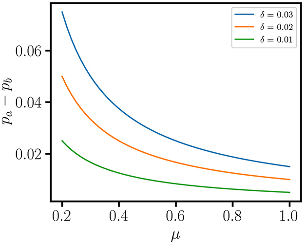
Figure 1. Proportional effects for a difference between mean values. Two mean values $(\overline{a},\overline{b})$ are associated with the center of mass coordinates $\left\{(\mu ,\delta /2)|\mu =(\overline{a}+\overline{b})/2,\delta =\overline{a}-\overline{b}\right\}$. Then, δ as a reduced representation for effect size is subject to ambiguity because of the loss of information when μ is ignored. This ambiguity is shown in the curves for the equivalence class of proportional effects, δ+2μ(p_b−p_a) = 0, for $(p_a,p_b)=(\overline{a},\overline{b})/(\overline{a}+\overline{b})$ and δ = {0.01, 0.02, 0.03}.

2.3.4 Covariance for the three pairwise data types

As discussed above, the three covariate data types are associated with distinct instrumental effects, algebraic problems, and covariance parameters. Therefore, we make the proposition:

Proposition 3. The distinct algebraic structures, parametric covariance vectors for LRVVs (× ^mℝⁿ) [22], the joint sort algorithm and nonoverlap proportion for point-biserial data $({\mathcal{C}}_2^n\times {ℝ}^n)$ [21], and 2 × 2 contingency tables for categorical data $({\mathcal{C}}_2^n\times {\mathcal{C}}_2^n)$ [16], result from the distinct additive and non-additive properties of numeric and categorical data, respectively. This implies that there are distinct forms of covariance and correlation for the three types of pairwise covariate data.

This has implications for Pearson's r [3]. We conclude that the implicit proposition that r, together with the $\mathcal{C}$₂-{0, 1}-numeric conversion procedure, serves as a unified correlation measure for numeric, categorical, and point-biserial data is false. The many-to-one grouping property of categorical data is incompatible with Pearson's r as a measure of linear dependence between VVs. This explains why ϕ [29] and rpb [30] do not serve as well-defined effect size measures in case-control data analysis, as shown in Fig 6A in [16] and Fig 6A,C in [21], respectively.

3 Results

In this section, we use MC simulations of heteroscedastic covariance to illustrate the instrumental properties of slope (Equation 26) and correlation (Equation 28) in PLR. This requires the specification of an error model for the data, $\mathcal{E}$($\mathcal{Y}$). Then, estimates for covariance and correlation parameters must be qualified with distributions and confidence intervals associated with $\mathcal{E}$($\mathcal{Y}$). However, fractional transformation, bounded range, and the discrete properties of categorical data complicate the development of analytical approaches for the propagation of error for ratios [41], correlation coefficients [42], and proportions [43]. Alternatively, MC methods allow the detailed simulation of stochastic effects [34, 44] in the data acquisition and the assessment of overdispersion in statistical parameters due to measurement errors: $\text{VAR}\left(y\right)=\text{VAR}\left(y^{*}\right)+\text{VAR}\left(e_y\right)$. This is important in correcting for bias in effect size analysis [45]. An MC simulation produces a distribution of datasets, $\mathcal{P}$($\mathcal{Y}$|$\mathcal{E}$($\mathcal{Y}$)),

$\begin{array}{ll}\left\{\mathcal{Y},ℰ(\mathcal{Y})\right\}\stackrel{\text{MC}}{\to }(\mathcal{Y}|ℰ(\mathcal{Y}))\to (v|ℰ(\mathcal{Y})).& (36)\end{array}$

Then, the corresponding distributions of statistical parameters, $\mathcal{P}$(v|$\mathcal{E}$($\mathcal{Y}$)), allows the estimation of distributions and confidence intervals for case-control covariance (Figure 5 in Luck [16]; Figure 7 in Luck [21]) and PLR parameters (Figure 4 in Luck [22]). Figure 2 shows results for MC simulations with evenly spaced fixed effects, {(x^*, y^*) ∈ (ℝ¹⁵ × ℝ¹⁵)|y^* = x^*+0.002, max(x^*) = 1} and varying dynamic range, DR ≡ max(x^*)/min(x^*), combined with independent normally distributed residual effects subject to quadratic variance error [22] $\left\{(e_x,e_y)|s_{x_i}^2=0.02\left(x_i^{*}+x_i^{{*}^2}\right),s_{y_i}^2=0.01\left(y_i^{*}+y_i^{{*}^2}\right)\right\}$. Three sets of data, $\left\{P_{\text{DR}}(x,y)|(x,y)=({\text{X}}^{*}+e_x,{\text{y}}^{*}+e_y)\right\},for\text{\hspace{0.17em}DR}=\{100,10,5\}$, for DR = {100, 10, 5} are obtained. For demonstration purposes, we use Equation 5 as the typical condition for instrumental performance. Then, the figures of merit for the W_x and W_y matrices are of the form,

$\begin{array}{ll}{c}_{y_i}^2=\frac{\left|y_i^{*}\right|}{s_{y_i^{*}}^2}.& (37)\end{array}$

This expression serves as an approximation, and it is not intended to serve as a general form for real applications. The figures of merit must reflect actual instrument performance and account for all relevant uncontrolled effects. In practice, CVE⁻¹ is replaced by signal-to-noise ratio, and $y_i^{*}$ is replaced by the signal value for y_i, including observations where y_i = 0. The data collection process must include replication, relevant control measurements, and error analysis required for assessing data quality [6]. The statistical parameters for the MC datasets are summarized in Table 1. The reliability ratios (${\kappa }_y=\text{Var}({\text{y}}^{*})/\text{Var}(\text{y})$ [46]) and CVEs increase with DR, but the optimum CVE weighting is invariant. Figure 2A shows the MC sample data for a single iteration with 2σ xy-error bars for the expected errors, {s_xi, s_yi}. The graphs in Figures 2B–D display the average values of PLR analysis parameters along with 2σ confidence intervals for 100,000 MC iterations. PLR parameters are estimated for a range of weighted averages, {τ_wx = w_xx+(1−w_x)y|0 ≤ w_x ≤ 1}, for each MC sample to obtain curves that illustrate the instrumental properties of slope and correlation. The optimal CVE estimates (listed in Table 1) are indicated by circles at w_x = 1/3. The curves in Figure 2B intersect at the point (1/3, 1) corresponding to the optimal PLR estimate for the slope, demonstrating the importance of adjusting for instrumental effects in the covariance. The endpoints of the concave-down curves for rPLRi in Figure 2C correspond to Pearson's r, demonstrating that r is attenuated by measurement error [22]. Comparison with rPLRw in Figure 2D shows that rPLRi is attenuated in the presence of heteroscedastic error. The distinct non-intersecting curves for varying DR in Figures 2C, D demonstrate that correlation coefficients are subject to instrumental effects. The larger confidence intervals in the PLR estimates for slope as DR → 1 result from the numerical instability as Var(x^*) → 0.

Table 1

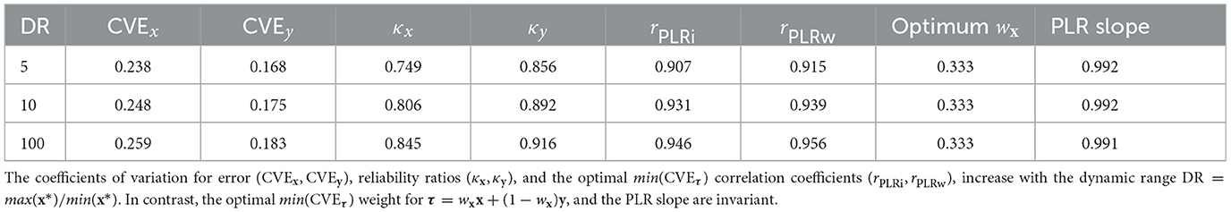
Table 1. Statistical parameters for the PLR simulations.

Figure 2

Figure 2. Instrumental properties of covariance and correlation in PLR. Monte Carlo simulations of heteroscedastic covariance for evenly spaced fixed data, (x^*, y^*) ∈ (ℝ¹⁵ × ℝ¹⁵) and y^* = x^*+0.002, combined with 10⁵ samples for independent normally distributed residual effects, $(\text{x},\text{y})=({\text{x}}^{*}+{\text{e}}_{\text{x}},{\text{y}}^{*}+{\text{e}}_{\text{y}})$, and quadratic variance error models for e_x, $s_{x_i}^2=0.02(x_i^{*}+x_i^{{*}^2})$, and e_y, $s_{y_i}^2=0.01(y_i^{*}+y_i^{{*}^2})$. Results are shown for three MC data sets with dynamic range, DR = {5, 10, 100}, where DR ≡ max(x^*)/min(x^*) and max(x^*) = 1. (A) (x, y) data for an MC sample with DR = 100 and 2σ xy-error bars for the expected errors (s_x, s_y). (B) Averages of PLR slope for heteroscedastic covariance (Equation 26) for weighted averages {τ = w_xx +(1−w_x)y|0 ≤ w_x ≤ 1}. The curves intersect at the point (0.333, 1.0) for the min(CVE_τ) optimum, demonstrating that the instrumental effects must cancel in dividing the WLS covariance by the corresponding variance to estimate the slope, (b_τx, b_τy) = [WCov(τ, x)/WVarx(τ), WCov(τ, y)/WVary(τ)]. The reliability ratios, (κ_x, κ_y), increase and the 2σ confidence intervals decrease with increasing DR. (C) The endpoints of the concave-down curves for homoscedastic rPLRi correspond to Pearson's r, demonstrating that r is attenuated by measurement error. (C, D) The distinct curves for DR = {5, 10, 100} demonstrate that rPLRi (Equation 7) and rPLRw (Equation 30) are instrumental quantities that depend on the spacings between data points and residual effects for linearly related variable vectors (LRVVs). The optimal min(CVE_τ) estimates are highlighted as circles. rPLRi does not account for heteroscedasticity and is biased downwards compared to rPLRw.

4 Discussion

The ordinary linear regression method requires the special homoscedastic condition for sample covariance. This work shows that we can achieve generalization through WLS optimization to account for heteroscedastic parametric covariance in PLR analysis. The application of weighted least squares methods for the normalization and analysis of RNA-Seq data is a topic for a future publication. In studies of complex systems, the inability to connect covariance parameters with the functional or model-dependent part of the inverse problem complicates the data analysis. This serves as motivation for the development of approximate methodologies, such as CART [18], to explore covariance in multivariate data and inform the creation of functional models for complex systems. However, in implementing the binary split algorithm in CART, it is necessary to account for all the degrees of freedom for the cost-benefit trade-offs in the case-control response. We conclude that instrumental effects, functionally ill-posed inverse problems, and tensor products for parametric covariance are important issues in covariate data analysis.

Data availability statement

The original contributions presented in the study are included in the article/supplementary material, further inquiries can be directed to the corresponding author.

Author contributions

SL: Methodology, Visualization, Conceptualization, Writing – original draft, Formal analysis, Software, Writing – review & editing, Investigation.

Funding

The author(s) declare that no financial support was received for the research and/or publication of this article.

Acknowledgments

I thank many former colleagues in the Genetic Discovery group at DuPont for many helpful discussions about genome-wide association and eQTL methods. I also especially thank my biologist collaborator and spouse, Ada Ching.

Conflict of interest

SL was employed by Vector Analytics LLC.

Generative AI statement

The author(s) declare that no Gen AI was used in the creation of this manuscript.

Any alternative text (alt text) provided alongside figures in this article has been generated by Frontiers with the support of artificial intelligence and reasonable efforts have been made to ensure accuracy, including review by the authors wherever possible. If you identify any issues, please contact us.

Publisher's note

All claims expressed in this article are solely those of the authors and do not necessarily represent those of their affiliated organizations, or those of the publisher, the editors and the reviewers. Any product that may be evaluated in this article, or claim that may be made by its manufacturer, is not guaranteed or endorsed by the publisher.

References

1. Tarantola A. Popper, Bayes and the inverse problem. Nat Phys. (2006) 2:492–4. doi: 10.1038/nphys375

Crossref Full Text | Google Scholar

2. Arridge S, Maass P, Öktem O, Schönlieb CB. Solving inverse problems using data-driven models. Acta Numerica. (2019) 28:1–174. doi: 10.1017/S0962492919000059

Crossref Full Text | Google Scholar

3. Rodgers JL, Nicewander WA. Thirteen ways to look at the correlation coefficient. Am Stat. (1988) 42:59–66. doi: 10.1080/00031305.1988.10475524

Crossref Full Text | Google Scholar

4. McGrath RE, Meyer GJ. When effect sizes disagree: the case of r and d. Psychol Methods. (2006) 11:386–401. doi: 10.1037/1082-989X.11.4.386

PubMed Abstract | Crossref Full Text | Google Scholar

5. VanLiere JM, Rosenberg NA. Mathematical properties of the r² measure of linkage disequilibrium. Theor Popul Biol. (2008) 74:130–7. doi: 10.1016/j.tpb.2008.05.006

PubMed Abstract | Crossref Full Text | Google Scholar

6. Cheng CL, Riu J. On estimating linear relationships when both variables are subject to heteroscedastic measurement errors. Technometrics. (2006) 48:511–9. doi: 10.1198/004017006000000237

PubMed Abstract | Crossref Full Text | Google Scholar

7. Saccenti E, Hendriks MHWB, Smilde AK. Corruption of the Pearson correlation coefficient by measurement error and its estimation, bias, and correction under different error models. Sci Rep. (2020) 10:438. doi: 10.1038/s41598-019-57247-4

PubMed Abstract | Crossref Full Text | Google Scholar

8. Kelley K, Preacher KJ. On effect size. Psychol Methods. (2012) 17:137–52. doi: 10.1037/a0028086

PubMed Abstract | Crossref Full Text | Google Scholar

9. Beló A, Zheng P, Luck S, Shen B, Meyer DJ, Li B, et al. Whole genome scan detects an allelic variant of fad2 associated with increased oleic acid levels in maize. Molec Genet Gen. (2008) 279:1–10. doi: 10.1007/s00438-007-0289-y

PubMed Abstract | Crossref Full Text | Google Scholar

10. Holloway B, Luck S, Beatty M, Rafalski JA, Li B. Genome-wide expression quantitative trait loci (eQTL) analysis in maize. BMC Gen. (2011) 12:336. doi: 10.1186/1471-2164-12-336

PubMed Abstract | Crossref Full Text | Google Scholar

11. Uffelmann E, Huang QQ, Munung NS, de Vries J, Okada Y, Martin AR, et al. Genome-wide association studies. Nat Rev Methods Primers. (2021) 1:59. doi: 10.1038/s43586-021-00056-9

Crossref Full Text | Google Scholar

12. Deshpande D, Chhugani K, Chang Y, Karlsberg A, Loeffler C, Zhang J, et al. RNA-seq data science: From raw data to effective interpretation. Front Genet. (2023) 14:997383. doi: 10.3389/fgene.2023.997383

PubMed Abstract | Crossref Full Text | Google Scholar

13. Brenner S. Sequences and consequences. Philos Trans R Soc London Series B, Biol Sci. (2010) 365:207–12. doi: 10.1098/rstb.2009.0221

PubMed Abstract | Crossref Full Text | Google Scholar

14. Pogrow S. How effect size (practical significance) misleads clinical practice: the case for switching to practical benefit to assess applied research findings. Am Stat. (2019) 73:223–34. doi: 10.1080/00031305.2018.1549101

Crossref Full Text | Google Scholar

15. Flora DB. Thinking about effect sizes: from the replication crisis to a cumulative psychological science. Canad Psychol. (2020) 61:318–30. doi: 10.1037/cap0000218

Crossref Full Text | Google Scholar

16. Luck S. Factoring a 2 x 2 contingency table. PLoS ONE. (2019) 14:e0224460. doi: 10.1371/journal.pone.0224460

PubMed Abstract | Crossref Full Text | Google Scholar

17. Rokach L, Maimon O. Data Mining with Decision Trees, vol. 81 London: World Scientific (2014). doi: 10.1142/9097

Crossref Full Text | Google Scholar

18. Krzywinski M, Altman N. Classification and regression trees. Nat Methods. (2017) 14:757–8. doi: 10.1038/nmeth.4370

Crossref Full Text | Google Scholar

19. Kuhn L, Page K, Ward J, Worrall-Carter L. The process and utility of classification and regression tree methodology in nursing research. J Adv Nurs. (2014) 70:1276–86. doi: 10.1111/jan.12288

PubMed Abstract | Crossref Full Text | Google Scholar

20. Schrodi SJ, Mukherjee S, Shan Y, Tromp G, Sninsky JJ, Callear AP, et al. Genetic-based prediction of disease traits: prediction is very difficult, especially about the future. Front Genet. (2014) 5:162. doi: 10.3389/fgene.2014.00162

PubMed Abstract | Crossref Full Text | Google Scholar

21. Luck S. Nonoverlap proportion and the representation of point-biserial variation. PLoS ONE. (2020) 15:e0244517. doi: 10.1371/journal.pone.0244517

PubMed Abstract | Crossref Full Text | Google Scholar

22. Luck S. A parametric framework for multidimensional linear measurement error regression. PLoS ONE. (2022) 17:e0262148. doi: 10.1371/journal.pone.0262148

PubMed Abstract | Crossref Full Text | Google Scholar

23. Evans C, Hardin J, Stoebel DM. Selecting between-sample RNA-Seq normalization methods from the perspective of their assumptions. Brief Bioinform. (2017) 19:776. doi: 10.1093/bib/bbx008

PubMed Abstract | Crossref Full Text | Google Scholar

24. Puntanen S, Styan GPH, Isotalo J. Matrix Tricks for Linear Statistical Models. Berlin Heidelberg: Springer (2011). doi: 10.1007/978-3-642-10473-2

Crossref Full Text | Google Scholar

25. Casella G, Berger R. Statistical Inference. 2 edn. Duxbury: Chapman and Hall/CRC (2002).

Google Scholar

26. Spiegelman D, Logan R, Grove D. Regression calibration with heteroscedastic error variance. Int J Biostat. (2011) 7:1259. doi: 10.2202/1557-4679.1259

PubMed Abstract | Crossref Full Text | Google Scholar

27. Romeo G, Buonaccorsi JP, Thoresen M. Detecting and correcting for heteroscedasticity in the presence of measurement error. Commun Stat Simul Comput. (2024) 53:5474–90. doi: 10.1080/03610918.2023.2190061

Crossref Full Text | Google Scholar

28. Gillard J, Iles T. Methods of fitting straight lines where both variables are subject to measurement error. Curr Clin Pharmacol. (2009) 4:164–71. doi: 10.2174/157488409789375302

PubMed Abstract | Crossref Full Text | Google Scholar

29. Hedrick PW. Gametic disequilibrium measures: proceed with caution. Genetics. (1987) 117:331–41. doi: 10.1093/genetics/117.2.331

PubMed Abstract | Crossref Full Text | Google Scholar

30. Kornbrot D. Point Biserial Correlation. New York: Wiley (2005). p. 1–3. doi: 10.1002/0470013192.bsa485

Crossref Full Text | Google Scholar

31. Balding DJ, A. tutorial on statistical methods for population association studies. Nat Rev Genet. (2006) 7:781–91. doi: 10.1038/nrg1916

PubMed Abstract | Crossref Full Text | Google Scholar

32. Noble B, Daniel JW. Applied Linear Algebra. 2nd edn. Boston: Prentice-Hall (1977).

Google Scholar

33. Draper NR, Smith H. Applied Regression Analysis. 3rd edn. New York: Wiley (1998). doi: 10.1002/9781118625590

Crossref Full Text | Google Scholar

34. Press WH Teukolsky SA Vetterling WT Flannery BP Press CU. Numerical Recipes: The Art of Scientific Computing. 3rd edn. Cambridge: Cambridge University Press (2007).

Google Scholar

35. Boyd SP, Vandenberghe L. Convex Optimization. Cambridge: Cambridge University Press (2004). doi: 10.1017/CBO9780511804441

Crossref Full Text | Google Scholar

36. Lebedev LP, Cloud MJ, Eremeyev VA. Tensor Analysis with Applications in Mechanics. Singapore: World Scientific (2010). doi: 10.1142/9789814313995

Crossref Full Text | Google Scholar

37. Jeevanjee N. An Introduction to Tensors and Group Theory for Physicists. Boston: Birkhäuser (2011). doi: 10.1007/978-0-8176-4715-5

Crossref Full Text | Google Scholar

38. Voigtman E. Comparison of signal-to-noise ratios. Anal Chem. (1997) 69:226–34. doi: 10.1021/ac960675d

Crossref Full Text | Google Scholar

39. Funder DC, Ozer DJ. Evaluating effect size in psychological research: sense and nonsense. Adv Methods Pract Psychol Sci. (2019) 2:156–68. doi: 10.1177/2515245919847202

Crossref Full Text | Google Scholar

40. Fritz CO, Morris PE, Richler JJ. Effect size estimates: current use, calculations, and interpretation. J Exper Psychol. (2012) 141:2–18. doi: 10.1037/a0024338

PubMed Abstract | Crossref Full Text | Google Scholar

41. von Luxburg U, Franz VH. A geometric approach to confidence sets for ratios: Fieller's theorem, generalizations, and bootstrap. Stat Sin. (2009) 19:1095–117. doi: 10.48550/arXiv.0711.0198

Crossref Full Text | Google Scholar

42. Bishara AJ, Hittner JB. Confidence intervals for correlations when data are not normal. Behav Res Methods. (2017) 49:294–309. doi: 10.3758/s13428-016-0702-8

PubMed Abstract | Crossref Full Text | Google Scholar

43. Agresti A. Dealing with discreteness: making ‘exact' confidence intervals for proportions, differences of proportions, and odds ratios more exact. Stat Methods Med Res. (2003) 12:3–21. doi: 10.1191/0962280203sm311ra

PubMed Abstract | Crossref Full Text | Google Scholar

44. Kroese DP, Brereton T, Taimre T, Botev ZI. Why the Monte Carlo method is so important today. WIREs Comput Statist. (2014) 6:386–92. doi: 10.1002/wics.1314

Crossref Full Text | Google Scholar

45. van Smeden M, Lash TL, Groenwold RHH. Reflection on modern methods: five myths about measurement error in epidemiological research. Int J Epidemiol. (2020) 49:338–47. doi: 10.1093/ije/dyz251

PubMed Abstract | Crossref Full Text | Google Scholar

46. Fuller WA. Measurement Error Models. New York: John Wiley & Sons, Inc. (2006).

Google Scholar