 Iman M. Attia
- Department of Mathematical Statistics, Faculty of Graduate Studies for Statistical Research, Cairo University, Giza, Egypt
Introduction: In this paper, the author presents the generalized form of the Median-Based Unit Rayleigh (MBUR) distribution, a novel statistical distribution that is specifically defined within the interval (0, 1). This generalization adds a new parameter to the MBUR distribution that significantly addresses the unique characteristics of data represented as ratios and proportions. The author considers a distinct technique for appending a new parameter to the unit distribution consuming the general formula for the order statistics.
Methods: The paper offers a thorough and meticulous derivation of the (PDF) for this distribution, illuminating each phase of the process with clarity and precision. It delves deep into the intricacies of the generalized odd MBUR (GOMBUR) distribution's properties, presenting a rigorous examination of the accompanying functions that are vital for robust statistical evaluation. These functions-comprising the (CDF), survival function, hazard rate, reversed hazard rate function, and raw moments.
Results and discussion: The paper discusses real data analysis and how the generalization improves such analysis. The author conducts a comparative analysis of the Generalized Odd Median Base Unit Rayleigh (GOMBUR) and the Median Based Unit Rayleigh (MBUR). The primary objective is to evaluate the additional benefits provided by the new shape parameter in the estimation process, focusing on various validity indices, goodness-of-fit statistics, estimated variances of the parameters, and their corresponding standard errors. Parameter estimation is performed using the Maximum Likelihood Estimator (MLE), with the Nelder-Mead optimization method employed for this purpose. The results obtained from this study can be summarized in the following points. (i) Incorporating new parameters into the MBUR model significantly enhances its flexibility, enabling it to accommodate a variety of data shapes with differing characteristics, such as skewness and kurtosis. (ii) This added parameter enhances the estimation process, resulting in improved validity indices, including (AIC), (CAIC), (BIC), and (HQIC). Additionally, it enhances the goodness of fit by reducing test statistics such as the (AD), (CVM), and (KS) tests, while increasing the Log-Likelihood. (iii) The two forms of the model yield different values for the parameter (n) but provide the same value for the parameter (alpha). The variances of the estimated (alpha) are identical, and the covariance between the parameters is minimal—significantly lower than that observed when fitting other distributions like the Beta and Kumaraswamy. Furthermore, the determinant of the estimated variance-covariance matrix from fitting the GOMBUR-1 model is among the lowest compared to those from the Beta and Kumaraswamy distributions.
1 Introduction
A multitude of real-world phenomena can be elegantly captured as proportions, ratios, or fractions nestled within the bounded interval (0, 1). These captivating representations are not merely abstract concepts; they reflect the intricate relationships found in various fields such as biology, where the delicate balance of ecosystems is analyzed; finance, where the flow of market ratios unfold; and mortality rates, which provide profound insights into human health and longevity. Additionally, recovery rates in medical science showcase the resilience of life, while economics delves into the nuanced distributions of wealth and resources. Engineering and hydrology further enrich this tapestry, modeling everything from structural integrity to the flow of water in our environments. The measurement sciences, too, rely on these continuous distributions, breathing life into data that inform our understanding of the world.
Some of these distributions include: the Johnson SB distribution [1], Beta distribution [2], Unit Johnson distribution [3], Topp-Leone distribution [4], Unit Gamma distribution [5–8], Unit Logistic distribution [9], Kumaraswamy distribution [10], Unit Burr-III distribution [11], Unit Modified Burr-III distribution [12], Unit Burr-XII distribution [13], Unit-Gompertz distribution [14], Unit-Lindley distribution [15], Unit-Weibull distribution [16], and Unit Muth distribution [17].
Generalizing a distribution by adding new parameters can undeniably enrich and amend the estimation process in numerous manners. First, adding parameters empowers the distribution to apprehend different data conducts such as skewness, kurtosis and different tail behaviors. For example, this is glorified when generalized gamma [18] distribution extends the gamma distribution to accommodate modeling wide range of data with different characteristics. The extra parameter in the generalized Pareto [19] distribution controlling the tail behavior facilitates it to better analyze the extreme values. Second, the newly added parameters amplify the goodness of fit to empirical data and reduce the systematic bias. An example for such an effect, when the data exhibit extreme values; the four parameter Beta distribution [20] extending the standard beta distribution can better model these heavy tail features data. Third, extending the distribution with new parameters augments it flexibility to align more properly with the basic data hence diminishing the bias in parameter estimation, obtaining more efficient estimators with minor variance and improve the implementation of MLE. The Generalized Weibull Distribution [21] enhances the estimates of failures rates in reliability studies. Fourth, the newly introduced parameters behave as regularizers that take control against over-fitting thereby improving stability in estimation. For example, the additional shape parameter in the Exponentiated Weibull Distribution [21] enables the modeling of both decreasing and increasing failure rates. Likewise, the skewness parameter in the Skew-Normal Distribution [22] promotes the distribution to better model the asymmetric data. Fifth, in real-world analysis like Generalized Logistic Distribution [23], implanting a shape parameter can regulate the rate of decay in growth models. The incorporated extra parameter in the Generalized Gamma [24] Distribution aids modeling diverse hazard rates.
The generalization of the unit distribution can be achieved through different mechanisms like power transformation to obtain the power Johnson B [25], power Generalized Johnson SB [26], and power unit inverse Lindley distribution [27]. The generalization can also be conducted using the T-X family method (transformed-transformer mechanism) like the transmuted power unit inverse Lindley distribution [28], Kumaraswamy generalized family of distribution [29], generalized distribution based on T-Topp -Leone family of distributions [30], and the generalized unit half logistic geometric distributions [31]. The author discusses in this paper a different method for adding a new parameter to the unit distribution using the general formula for the order statistics.
It's important to recognize the limitations of this generalization. While adding more parameters can enhance a model's complexity and capability, it also brings challenges that must be carefully considered. Increased parameters may complicate computations and require sophisticated optimization techniques to manage effectively. Additionally, a larger set of parameters can introduce identifiability issues, where the effects of certain parameters become unclear. Many parameters may even lack practical significance, questioning their value in real-world applications. Therefore, it's crucial to weigh the advantages of incorporating new parameters against the potential difficulties they could introduce, ensuring that we make informed decisions in our modeling approaches.
This paper is structured into several sections for clarity and coherence. Section 2 provides a comprehensive discussion of the methodology employed to derive the new distribution. Section 3 delves into its fundamental characteristics, including the probability density function (PDF), cumulative distribution function (CDF), survival function (S), hazard function (HF), reversed hazard function (RHF), and quantile function. Section 4 demonstrates the maximum likelihood estimation method. Section 5 offers an in-depth discussion that encompasses an analysis of real data as well as a detailed examination of the findings. In conclusion, Section 6 provides a comprehensive overview of our findings and offers valuable recommendations for future research, inviting further exploration and innovation in the field.
2 Methodology
2.1. Derivation of the PDF
The general formula of the median order statistics for an odd sample size can be written as in Equation 1.
Where (i) is the ith odd order statistics and m is the sample size. Replacing (m) sample size (which is an odd number) with m = 2n + 1 as shown in Equations 2.A and 2.B.
Substituting Equation 3 which is the CDF and the PDF of Rayleigh distribution in Equation 2.B yields Equation 4.
Using the transformation in Equation 5 and the Jacobian in Equation 6 and then substituting both in Equation 4 yields the new PDF in Equation 7. This is the first version of generalization of the MBUR.
The second version of generalization is obtained by substituting the CDF and the PDF of Rayleigh in Equation 8 which yields Equation 9
Substituting the same transformation of Equation 5 and the same Jacobian of Equation 6 in Equation 9 yields the new PDF in Equation 10. This is the second version of generalization of the MBUR distribution.
Theorem 1: Both versions in Equations 7 and 10 are valid PDF.
Proof: PDF version in Equation 7:
To prove that the PDF in Equation 7 is a valid PDF, the integral in Equation 11 should equal 1. Applying the transformation in Equation 12 and substitute in Equation 11:
For the PDF version in Equation 10, applying the same transformation will integrate the PDF in Equation 10 to 1.
3 Some properties of the generalized odd MBUR distribution
Theorem 2: the cumulative distribution function (CDF) of the generalized odd MBUR is:
P(Y < y) = Iw(n+1, n+1) for version 1 and for version 2.
Proof: for version 1:
Apply the transformation of Equation 12 and substitute in Equation 13 yields Equation 14
For version 2:
Apply the transformation of Equation 12 and substitute in equation 15 yields Equation 16
Lemma 1: the survival function (S) for version 1 is shown in Equation 17
Lemma 2: the survival function (S) for version 2 is shown in Equation 18
Lemma 3: The Hazard function or rate (HF or hr) for version 1 is shown in Equation 19
Lemma 4: The Hazard function or rate (HF or hr) for version 2 is shown in Equation 20
Lemma 5: the reversed hazard function (RHF) or reversed hazard rate (rhr) for version 1 is shown in Equation 21
Lemma 6: the reversed hazard function (RHF) or reversed hazard rate (rhr) for version 2 is shown in Equation 22
The quantile function of the distribution has no closed explicit form.
Theorem 3: the rth raw moment of the first version of the distribution is given by
Proof: the expectation of the rth moment in Equation 23 is obtained with the help of the transformation mentioned in Equation 12
Theorem 4: the rth raw moment of the second version of the distribution is given by
Proof: the expectation of the rth moment in Equation 24 is obtained with the help of the transformation mentioned in Equation 12
Figures 1–4 show PDF, CDF, survival function, Hazard function for the distribution at different parameters values. See Supplementary material 1 for more figures.
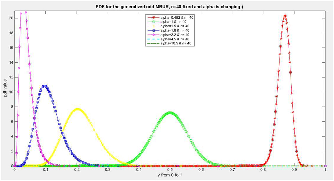
Figure 1. Shows PDF of the first version for different levels of alpha and n = 40.
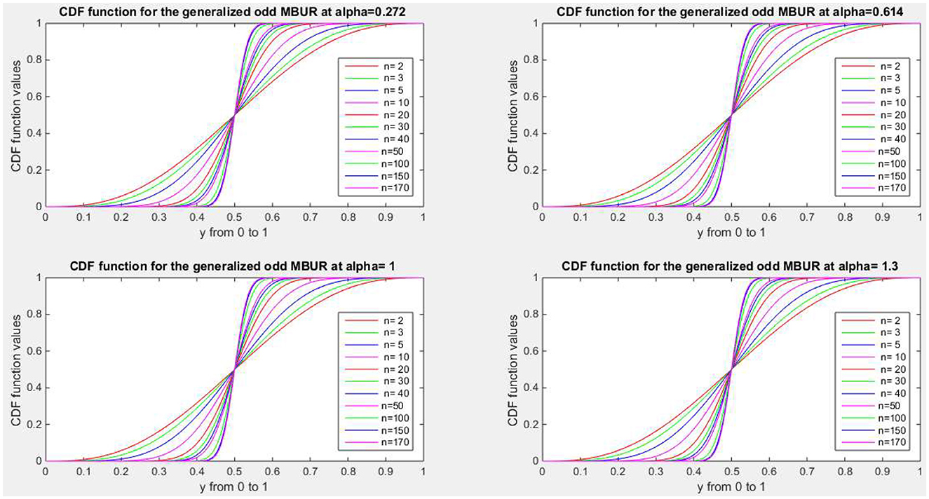
Figure 2. Shows CDF of the first version for different levels of alpha and n.
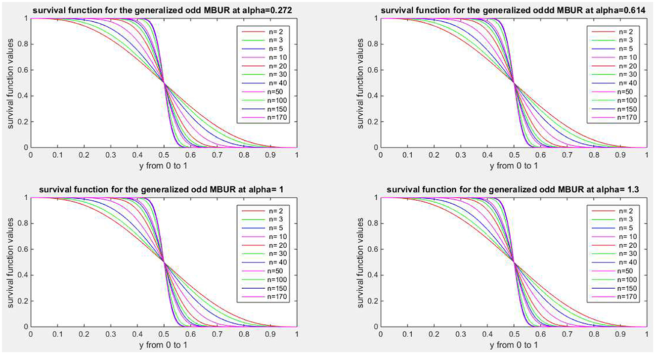
Figure 3. Shows survival function of the first version for different levels of alpha and n.
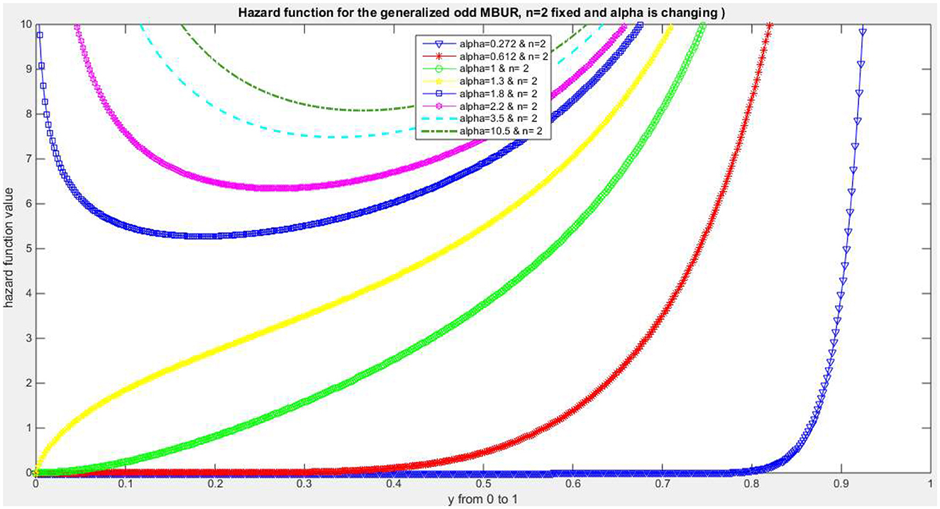
Figure 4. Shows hazard rate function of the first version for different levels of alpha and n = 2.
4 Methods of estimation
4.1 Maximum likelihood estimation
Let Y be a random variable having the PDF of GOMBUR-1. To derive the MLE for version 1, for one observation, taking the log of Equation 7 results in Equation 25:
Taking the first derivative of Equation 25 with respect to n and alpha parameter yields Equations 26 and 27, respectively:
Let Y be a random variable having the PDF of GOMBUR-2. To derive the MLE for version 2, for one observation, taking the log of Equation 10 results into Equation 28:
Taking the first derivative of Equation 28 with respect to n and alpha parameter yields Equations 29 and 30, respectively:
For each version, set the above equations to zero, and since they are non-linear equations, numerical methods like quasi-Newton method can be used as a solution.
5 Real data analysis
5.1. Description of the real data
The real data used in this paper can be found in Appendix A in Supplementary material 2. These are 14 datasets. In the main manuscript, the author will discuss only two of them. The flood dataset was used by the author [32] in previous work. The second dataset is the COVID-19 death rate in Canada, previously analyzed by [33].
The analysis of the data sets aims to determine how these sets correspond to the following distributions: Beta, Topp-Leone, Unit Lindley, and Kumaraswamy. The author will compare the fitting of these data sets to the fitting of the new MBUR distribution [32] and its generalized forms, GOMBUR-1 and GOMBUR-2. The evaluation will utilize several metrics, including the log-likelihood (LL), Akaike Information Criterion (AIC), corrected AIC (CAIC), Bayesian Information Criterion (BIC), and Hannan-Quinn Information Criterion (HQIC). Additionally, the author will perform the Kolmogorov-Smirnov (K-S) test, documenting its value as well as the outcome of the null hypothesis (H0), which posits that the data set follows the investigated distribution. If the data do not support this assumption, the null hypothesis is rejected. The P-value for the test will also be recorded. Furthermore, the Cramér-von Mises test and the Anderson-Darling test will be conducted, with their respective values reported. Figures illustrating the empirical cumulative distribution function (eCDF) and the theoretical cumulative distribution functions (CDF) of the distributions will be included. The author will present the estimated parameter values, along with their variances and standard errors. MATLAB was used for analysis. The competing distributions are as follows:
1- Beta Distribution:
2- Kumaraswamy Distribution: f(y; α, β) = , 0 < y < 1, α>0, β> 0
3- Median Based Unit Rayleigh:
4- Topp-Leone Distribution: f(y; θ) = , 0 < y < 1, θ> 0
5- Unit-Lindley:
Comparison tools are: (k) is the number of parameter, (n) is the number of observations.
5.2 Descriptive statistics of the datasets
Figure 5 and Table 1 shows that the flood data are right skewed and exhibits excess kurtosis (leptokurtic) while the COVID-19 death rate in Canada data rate are slightly left skewed and exhibit less than excess kurtosis (platykurtic).
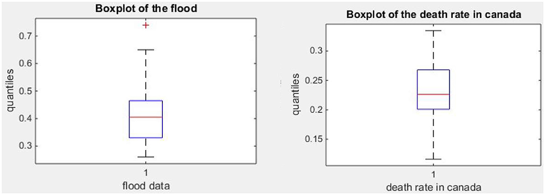
Figure 5. Boxplot of the flood data and COVID-19 death rate in Canada.

Table 1. Illustrates the descriptive statistics for the above datasets.
5.3 Individual dataset analysis (results and discussion)
For each dataset, there will be a table displaying the results of the fitted distributions, along with figures that highlight the fitted (CDFs) and (PDFs) for the tested distributions. An extra figure will be provided to compare the fitted CDFs and PDFs of the two versions. Tables 2A, 2B presents the results of the analysis of the flood data with accompanied Figures 6–8.
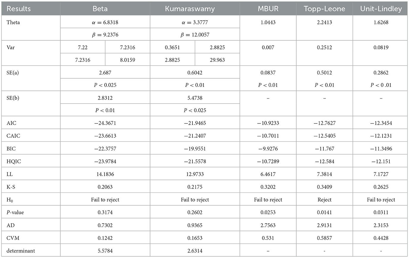
Table 2A. Shows the results of analysis of flood data.
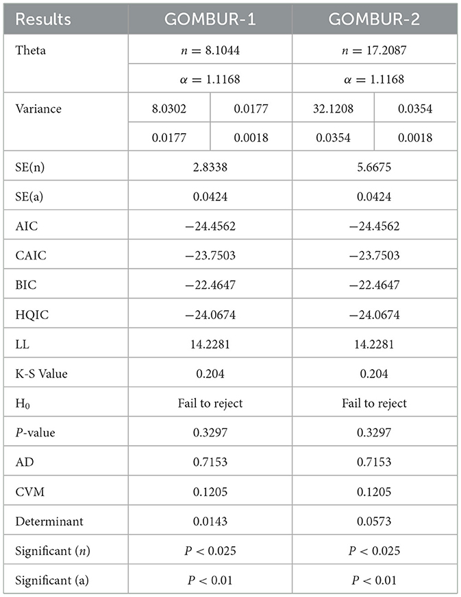
Table 2B. To be continued: comparison between GOMBUR 1 and GOMBUR 2.
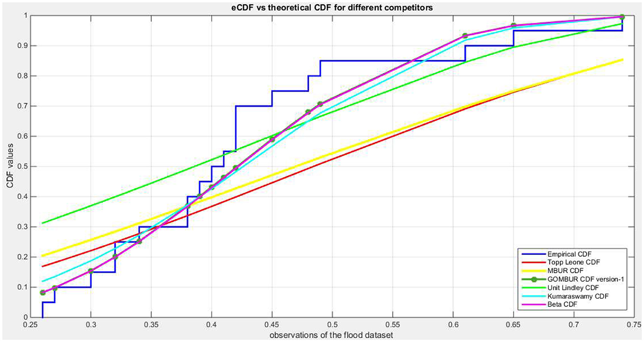
Figure 6. Shows the e-CDF and the theoretical CDF for the fitted distributions of flood data.
The analysis shows that Beta distribution fits the data better than any other distribution. The Topp Leone did not fit the distribution. Generalization of MBUR using the GOMBUR-1 improves the fitting up to the level of the Beta distribution and slightly exceeding it. Marked increases in the negativity levels of AIC, CAIC, BIC & HQIC are obtained. The level of Log-likelihood shows marked improvement. Marked reduction in the levels of AD and CVM statistics are obvious. The variance of the estimated alpha shows marked reduction after fitting the GOMBUR-1. The determinant of GOMBUR-1&2 is far less than the determinant of the Beta distribution and Kumaraswamy distribution demonstrating more efficiency. GOMBUR-1 has lesser determinant than the GOMBUR-2. The estimates of alpha value, their variances and standard errors are identical for both versions. While the estimates of the n parameter, its variance and standard error obtained after fitting GOMBUR-2 is higher than the levels obtained after fitting GOMBUR-1 distribution.
Figure 6 shows the eCDF and the theoretical CDF for the fitted distributions. Figure 7 shows the fitted PDFs. Figure 8 illuminates the fitted CDFs and the fitted PDFs for both versions of the generalization expounding identity of the curves.
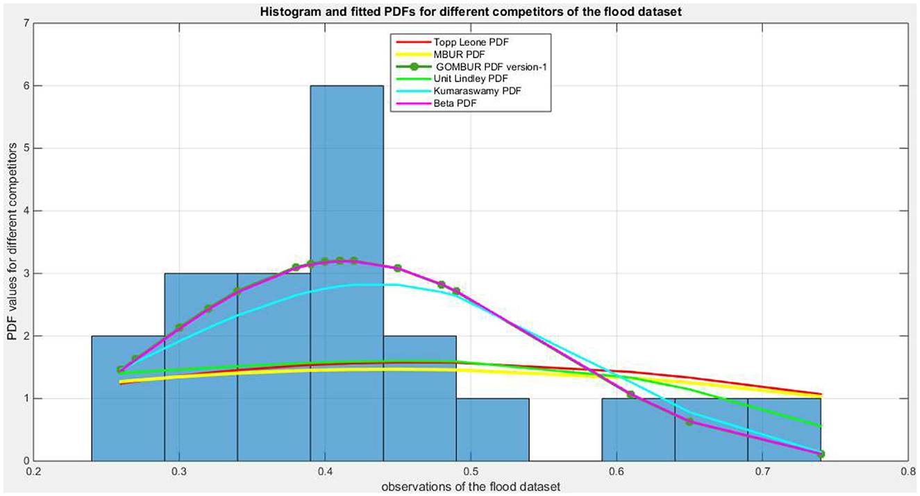
Figure 7. Shows the histogram of the flood data and the theoretical PDFs for the fitted distributions. The GOMBUR-1 perfectly aligns with the Beta distribution.
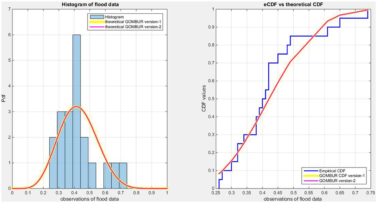
Figure 8. Shows on the left subplot the histogram of the flood data and the fitted PDFs of both GOMBUR-1 and GOMBUR-2 and on the right subplot the e-CDF and the theoretical CDF for both distributions. Both the fitted CDF and the fitted PDFs of both versions are identical.
The next data is the COVID-19 death rate in Canada. The results are shown in Tables 3A, 3B with associated Figures 9–11.
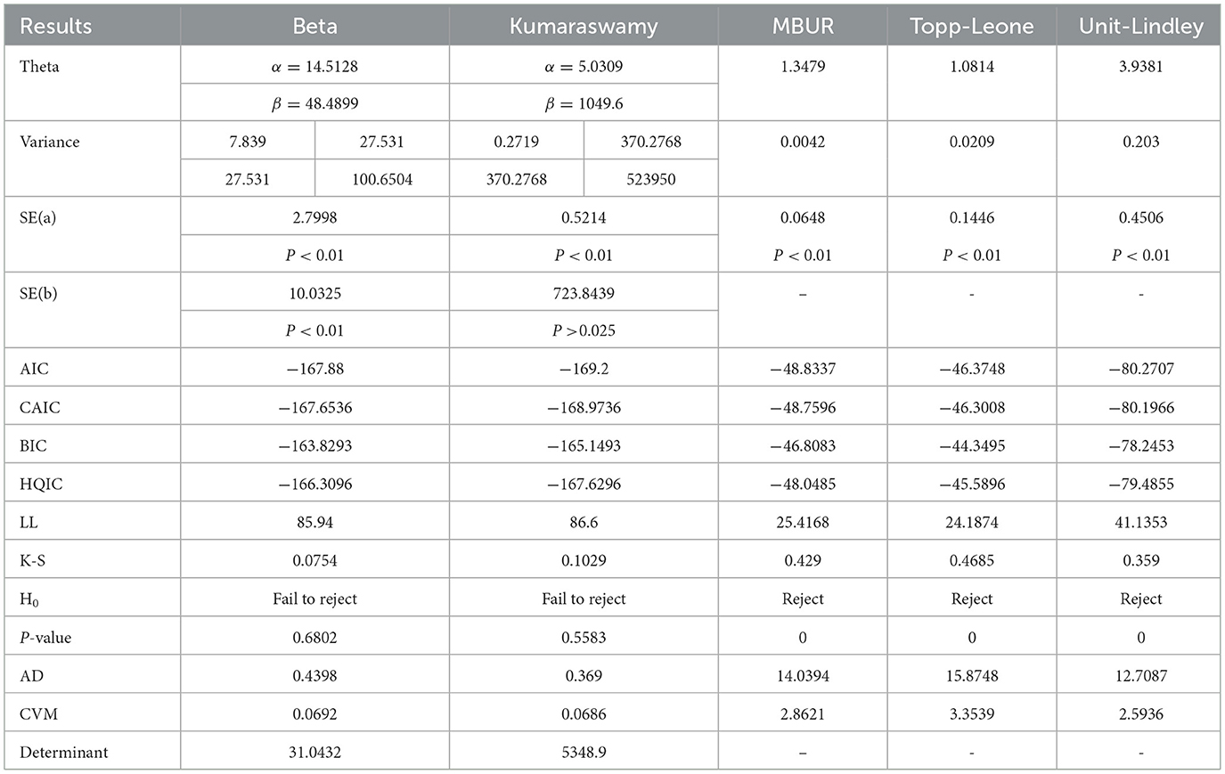
Table 3A. Shows the results of analysis of COVID-19 death rate analysis in Canada.
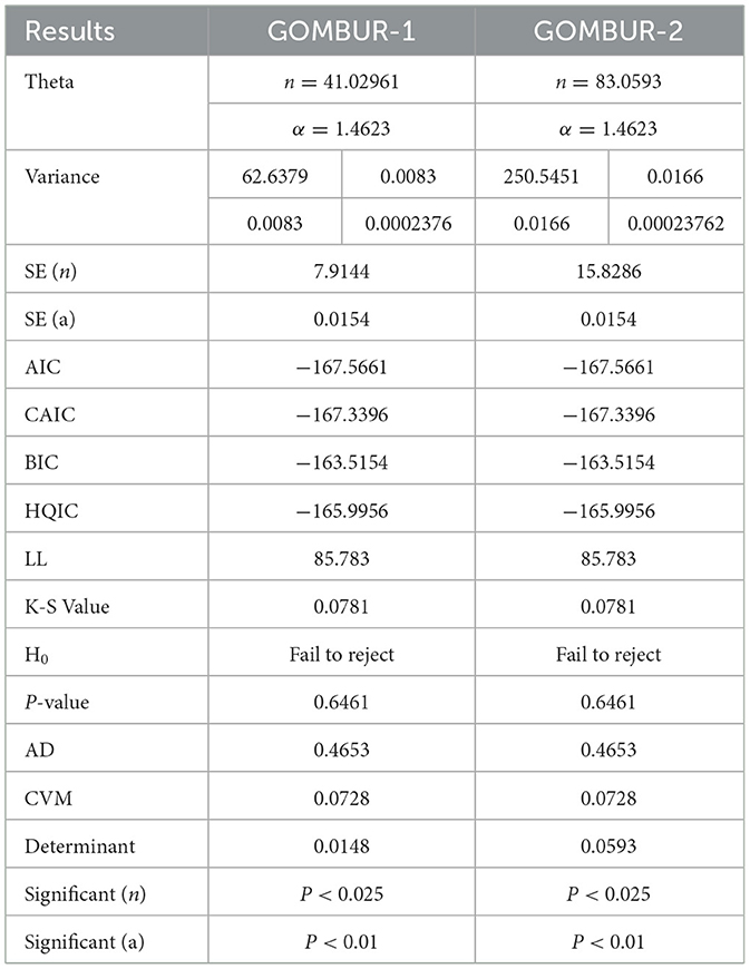
Table 3B. To be continued: comparison between GOMBUR 1 and GOMBIR 2.
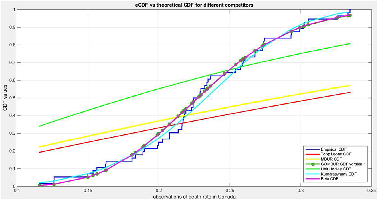
Figure 9. Shows the e-CDF and the theoretical CDF for the fitted distributions of death rate in Canada data.
The analysis indicates that both the Beta distribution and the Kumaraswamy distribution provide a good fit for the data. In contrast, the MBUR, Topp Leone, and Unit Lindley distributions do not fit the data well. The GOMBUR-1 and GOMBUR-2 distributions fit the data adequately, with their AIC, CAIC, BIC, and HQIC values significantly outperforming those of MBUR, although they are slightly less effective than the Kumaraswamy and Beta distributions. One key advantage of using the generalized form of MBUR is that it reduces variance, as demonstrated by the notably lower values of the determinants of the variance-covariance matrices obtained after fitting the GOMBUR-1 and GOMBUR-2 distributions. The estimated variance for alpha is significantly lower than that obtained from fitting the Beta and Kumaraswamy distributions. Additionally, the estimated alpha levels, their variances, and standard errors are consistent across both versions of the GOMBUR distributions. Although the Kumaraswamy fitting shows more negative values for AIC, BIC, and HQIC—indicating superior performance compared to both the Beta and GOMBUR-1 data fittings—it also has a higher value for the determinant of the variance-covariance matrix, leading to a less efficient fit of the data.
Figure 9 show the eCDF and theoretical CDF for the fitted distributions. Figure 10 depicts the fitted PDF. While Figure 11 displays the fitted (CDFs) and the fitted (PDFs) for both versions. The shapes of the PDFs are symmetrical and identical for both versions, which is expected given the large estimated values of “n.” Generally, as the estimated “n” increases, the distribution becomes more symmetrical.
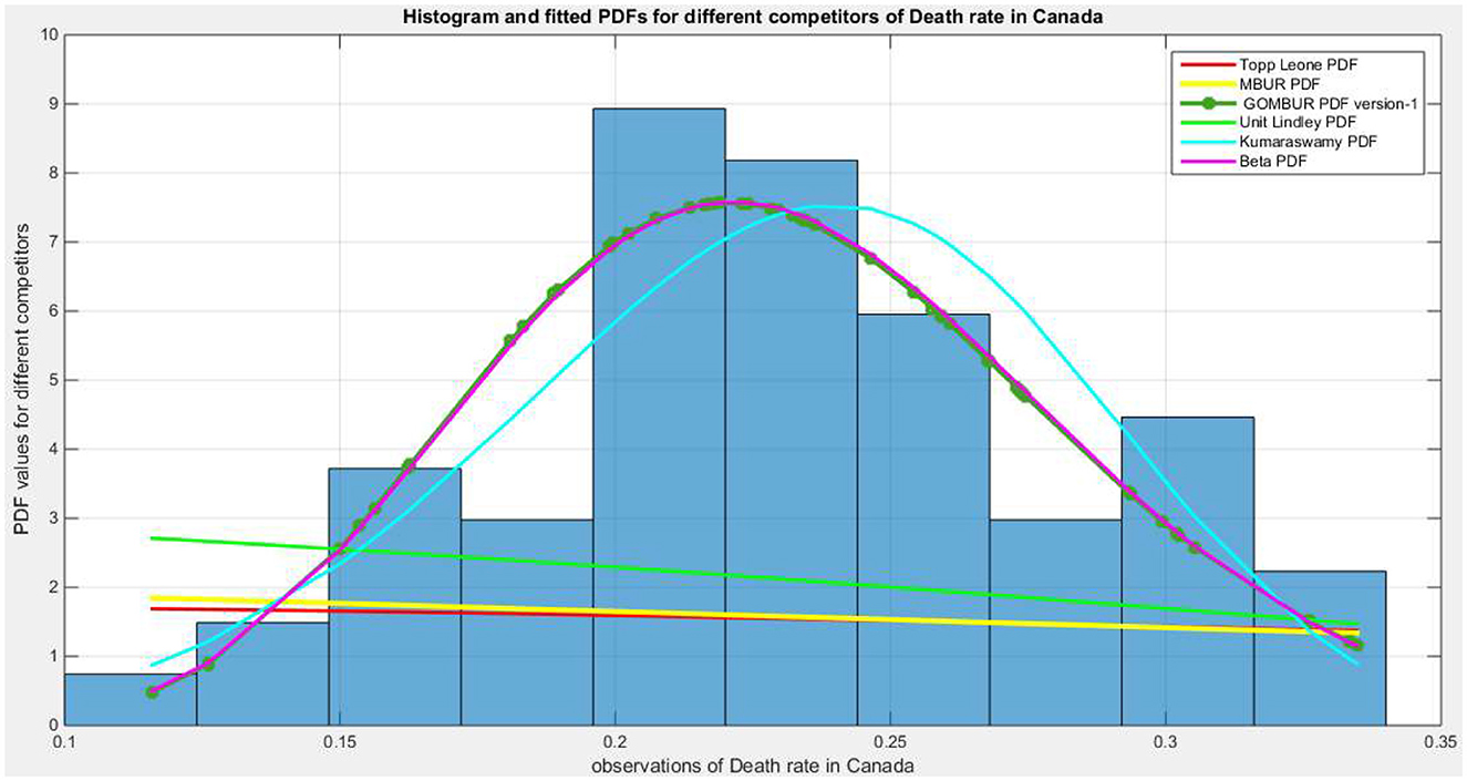
Figure 10. Shows the histogram of the COVID-19 death rate in Canada data and the theoretical PDFs for the fitted distributions. The GOMBUR-1 shows near-perfect alignments with Beta distribution. Kumaraswamy distribution fits the data. MBUR, Topp Leone, Unit Lindley distributions do not fit the data.
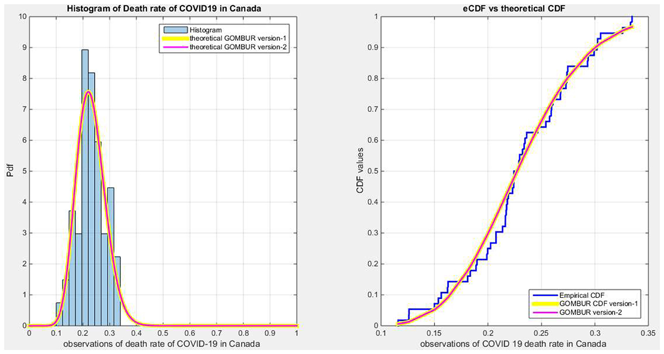
Figure 11. Shows on the left subplot the histogram of the death rate in Canada data and the fitted PDFs of both GOMBUR-1 and GOMBUR-2 and on the right subplot the e-CDF and the theoretical CDF for both distributions. Both the fitted CDF and the fitted PDFs of both versions are identical.
6 Conclusion
The addition of a new parameter to the previously studied MBUR distribution enhances the capability of MBUR to fit the data. Two versions for generalizing the MBUR were discussed by the author. Both have a non-explicit closed form of the CDF, but they can be expressed using special function. Subsequently, the quantile functions for both versions are not expressed in closed form. Also the rth moments of both versions are expressed with the aid of special function. This is considered as a limitation for being used in applications like median based quantile regression or mean based regression in generalized linear model. The advantage of adding this new parameter is that it helps MBUR to fit near symmetric data. Moreover, the two versions of this Generalized Odd MBUR exhibit a new shape for the hazard rate in the form of an oscillating pattern at the end of the distribution before approaching infinity and at different values of the random variable depending on the level of the alpha and the n parameter (See Supplementary materials 1).
The analysis of the datasets shows that adding a new parameter to the MBUR model increases its flexibility, allowing it to accommodate diverse shapes of data with different characteristics, such as skewness, kurtosis, and various tail behaviors. This newly introduced parameter enhances the estimation process by improving validity indices like AIC, CAIC, BIC, and HQIC. Additionally, it enhances the goodness of fit by reducing test statistics such as the (AD), (CVM), and (KS) tests. Furthermore, it increases the value of the Log-Likelihood. The two versions of the generalization yield different values for the parameter (n), but they have equal values for the parameter (alpha). The variances of the estimated (alpha) obtained from the two versions are identical, and the covariance between the two parameters is minimal, which is significantly lower than the covariance observed when fitting distributions like the Beta and the Kumaraswamy. The determinant of the estimated variance-covariance matrix obtained from fitting GOMBUR-1 is minimal, almost the lowest compared to that achieved after fitting the Beta and Kumaraswamy distributions. In Supplementary material 3, the author discusses various new generalized unit distributions utilizing the general formula for the order statistics. These distributions can be candidates for various applications in future work.
7 Future work
In this paper, the Nelder-Mead optimizer was employed for Maximum Likelihood Estimation (MLE) of the parameters. Future work may explore Bayesian inference procedures. Methods like Maximum product of spacing, least square and weighted least square methods can be attempted but the encountered limitation is that the CDF does not have a well-closed form. This limitation will impose some cumbersome calculations to estimate the parameters. The generalized method of moments using moment based approach by equating the sample moments with the population moments can offer an alternative for parameter estimation. But this will also face some difficult calculations as the moments require special functions. Applying derivative based algorithms like Quasi-Newton methods could be another solution for the optimization procedure.
Data availability statement
The original contributions presented in the study are included in the article/Supplementary material, further inquiries can be directed to the corresponding author.
Author contributions
IA: Conceptualization, Data curation, Formal analysis, Funding acquisition, Investigation, Methodology, Project administration, Resources, Software, Supervision, Validation, Visualization, Writing – original draft, Writing – review & editing.
Funding
The author(s) declare that no financial support was received for the research and/or publication of this article.
Conflict of interest
The author declares that the research was conducted in the absence of any commercial or financial relationships that could be construed as a potential conflict of interest.
Generative AI statement
The author(s) declare that no Gen AI was used in the creation of this manuscript.
Any alternative text (alt text) provided alongside figures in this article has been generated by Frontiers with the support of artificial intelligence and reasonable efforts have been made to ensure accuracy, including review by the authors wherever possible. If you identify any issues, please contact us.
Publisher's note
All claims expressed in this article are solely those of the authors and do not necessarily represent those of their affiliated organizations, or those of the publisher, the editors and the reviewers. Any product that may be evaluated in this article, or claim that may be made by its manufacturer, is not guaranteed or endorsed by the publisher.
Supplementary material
The Supplementary Material for this article can be found online at: https://www.frontiersin.org/articles/10.3389/fams.2025.1648127/full#supplementary-material
References
1. Johnson NL. Systems of frequency curves generated by methods of translation. Biometrika. (1949) 36:149–76. doi: 10.1093/biomet/36.1-2.149
2. Eugene N, Lee C, Famoye F. Beta-normal distribution and its applications. Commun Statist - Theory Methods. (2002) 31:497–512. doi: 10.1081/STA-120003130
3. Gündüz S, Korkmaz MÇ. A new unit distribution based on the unbounded johnson distribution rule: the unit Johnson SU distribution. Pak J Stat Oper Res. (2020) 16:471–90. doi: 10.18187/pjsor.v16i3.3421
4. Topp CW, Leone FC. A family of J-shaped frequency functions. J Am Stat Assoc. (1955) 50:209–19. doi: 10.1080/01621459.1955.10501259
5. Consul PC, Jain GC. On the log-gamma distribution and its properties. Statistische Hefte. (1971) 12:100–6. doi: 10.1007/BF02922944
6. Grassia A. On a family of distributions with argument between 0 and 1 obtained by transformation of the gamma and derived compound distributions. Austral J Stat. (1977) 19:108–14. doi: 10.1111/j.1467-842X.1977.tb01277.x
7. Mazucheli J, Menezes AFB, Dey S. Improved maximum-likelihood estimators for the parameters of the unit-gamma distribution. Commun Stat - Theory Methods. (2018) 47:3767–78. doi: 10.1080/03610926.2017.1361993
8. Tadikamalla PR. On a family of distributions obtained by the transformation of the gamma distribution. J Stat Comput Simul. (1981) 13:209–14. doi: 10.1080/00949658108810497
9. Tadikamalla PR, Johnson NL. Systems of frequency curves generated by transformations of logistic variables. Biometrika. (1982) 69:461–5. doi: 10.1093/biomet/69.2.461
10. Kumaraswamy P. A generalized probability density function for double-bounded random processes. J Hydrol. (1980) 46:79–88. doi: 10.1016/0022-1694(80)90036-0
11. Modi K, Gill V. Unit Burr-III distribution with application. J Stat Manag Syst. (2020) 23:579–92. doi: 10.1080/09720510.2019.1646503
12. Haq MAU, Hashmi S, Aidi K, Ramos PL, Louzada F. Unit Modified Burr-III distribution: estimation, characterizations and validation test. Ann Data Sci. (2023) 10:415–40. doi: 10.1007/s40745-020-00298-6
13. Korkmaz MÇ, Chesneau C. On the unit Burr-XII distribution with the quantile regression modeling and applications. Comput Appl Math. (2021) 40:29. doi: 10.1007/s40314-021-01418-5
14. Mazucheli J, Maringa AF, Dey S. Unit-Gompertz distribution with applications. Statistica. (2019) 79:25–43. doi: 10.6092/ISSN.1973-2201/8497
15. Mazucheli J, Menezes AFB, Chakraborty S. On the one parameter unit-Lindley distribution and its associated regression model for proportion data. J Appl Stat. (2019) 46:700–14. doi: 10.1080/02664763.2018.1511774
16. Mazucheli J, Menezes AFB, Fernandes LB, De Oliveira RP, Ghitany ME. The unit-Weibull distribution as an alternative to the Kumaraswamy distribution for the modeling of quantiles conditional on covariates. J Appl Stat. (2020) 47:954–74. doi: 10.1080/02664763.2019.1657813
17. Maya R, Jodrá P, Irshad MR, Krishna A. The unit Muth distribution: statistical properties and applications. Ricerche Di Matematica. (2024) 73:1843–66. doi: 10.1007/s11587-022-00703-7
18. Kiche J, Ngesa O, Orwa G. On generalized gamma distribution and its application to survival data. Int J Stat Prob. (2019) 8:85. doi: 10.5539/ijsp.v8n5p85
19. Malik MR, Kumar D. Generalized pareto distribution based on generalized order statistics and associated inference. Stat Trans New Ser. (2019) 20:57–79. doi: 10.21307/stattrans-2019-024
20. McGarvey RG, Del Castillo E, Cavalier TM, Lehtihet EA. Four-parameter beta distribution estimation and skewness test. Qual Reliab Eng Int. (2002) 18:395–402. doi: 10.1002/qre.490
21. Shama MS, Alharthi AS, Almulhim FA, Gemeay AM, Meraou MA, Mustafa MS, et al. Modified generalized Weibull distribution: theory and applications. Sci Rep. (2023) 13:12828. doi: 10.1038/s41598-023-38942-9
22. Arellano-Valle RB, Azzalini A. Some properties of the unified skew-normal distribution. Stat Papers. (2022) 63:461–87. doi: 10.1007/s00362-021-01235-2
23. Aljarrah MA, Famoye F, Lee C. Generalized logistic distribution and its regression model. J Stat Distrib Applic. (2020) 7:7. doi: 10.1186/s40488-020-00107-8
24. Gupta RD, Kundu D. Theory and methods: generalized exponential distributions. Austral N Zeal J Stat. (1999) 41:173–88. doi: 10.1111/1467-842X.00072
25. Cancho VG Bazán JL and Dey DK. A new class of regression model for a bounded response with application in the study of the incidence rate of colorectal cancer. Stat Methods Med Res. (2020) 29:2015–33. doi: 10.1177/0962280219881470
26. Gallardo DI, Bourguignon M, Gómez YM. Caaman̄o-Carrillo C, and Venegas O. Parametric quantile regression models for fitting double bounded response with application to COVID-19 mortality rate data. Mathematics. (2022) 10, 2249. doi: 10.3390/math10132249
27. Gemeay AM Alsadat N Chesneau C and Elgarhy M. Power unit inverse Lindley distribution with different measures of uncertainty, estimation and applications. MATH. (2024) 9:20976–024. doi: 10.3934/math.20241021
28. Eldessouky EA Hassan OHM Aloraini B and Elbatal I. Modeling to medical and economic data using: The transmuted power unit inverse Lindley distribution. Alexandria Eng J. (2025) 113:633–47. doi: 10.1016/j.aej.2024.11.008
29. Tahir MH Hussain MA Cordeiro GM El-Morshedy M and Eliwa MS. A new kumaraswamy generalized family of distributions with properties, applications, and bivariate extension. Mathematics, (2020) 8, 1989. doi: 10.3390/math8111989
30. Sudsila P Thongteeraparp A Aryuyuen S and Bodhisuwan W. The generalized distributions on the unit interval based on the T-Topp-Leone family of distributions. Trends Sci. (2022) 19, 6186. doi: 10.48048/tis.2022.6186
31. Nasiru S Chesneau C Abubakari AG and Angbing ID. Generalized unit half-logistic geometric distribution: properties and regression with applications to insurance. Analytics, (2023) 2:438–462. doi: 10.3390/analytics2020025
32. Attia MI. A novel unit distribution named as Median Based Unit Rayleigh (MBUR):properties and estimations. Preprints.Org (2024). doi: 10.36227/techrxiv.172840539.93243038/v1
Keywords: generalized odd MBUR, Median Based Unit Rayleigh, maximum likelihood estimator, hazard rate function, COVID-19 death rate in Canada
Citation: Attia IM (2025) The new generalized odd Median Based Unit Rayleigh. Front. Appl. Math. Stat. 11:1648127. doi: 10.3389/fams.2025.1648127
Received: 19 June 2025; Accepted: 03 September 2025;
Published: 08 October 2025.
Edited by:
Nossaiba Baba, University of Hassan II Casablanca, MoroccoReviewed by:
Hajar Nafia, University of Hassan II Casablanca, MoroccoKhalaf H. Habib, Tikrit University, Iraq
Copyright © 2025 Attia. This is an open-access article distributed under the terms of the Creative Commons Attribution License (CC BY). The use, distribution or reproduction in other forums is permitted, provided the original author(s) and the copyright owner(s) are credited and that the original publication in this journal is cited, in accordance with accepted academic practice. No use, distribution or reproduction is permitted which does not comply with these terms.
*Correspondence: Iman M. Attia, aW1hbmF0dGlhdGhlc2lzMTk3MkBnbWFpbC5jb20=