Estimating and testing blip effects of treatments in sequence via standardized point effects of treatments

In longitudinal studies, treatments are often assigned in the form of a sequence to achieve a certain outcome of interest. The blip effect of treatment in sequence is the net effect of treatment on the outcome. In this article, we introduce a method of estimating and testing the blip effects via the standardized point effects of treatments in sequence. First, we apply available methods to estimate the point effects referring to single-point treatments. Then we standardize the point effects to a small number of strata of relevance to the blip effects of interest. Finally, we use the standardized point effects to estimate and test the blip effects. Our method addresses two issues in complex longitudinal studies: a dimension reduction without strict treatment assignment conditions and a targeted analysis of the blip effects of interest across different times. The simulation study shows that our method achieves unbiased estimates of the blip effect, maintains nominal coverage probability, and demonstrates high power for hypothesis testing. A medical example illustrates the application of our method in observational studies.

1 Introduction

In many medical practices, treatments are assigned in the form of a sequence to achieve a certain outcome of interest. Besides stationary covariates, there are often time-dependent covariates between treatments, which may have influences from the earlier treatments and on the subsequent treatments. From the observed treatments, covariates, and outcome, one wishes to estimate the causal effect of a specified regime of treatments on the outcome. A special type of such causal effects is the blip effect of treatment in sequence, which is the causal effect of treatment given all the previous treatments and covariates, while the subsequent treatments are set at controls [1]. The blip effect describes the net effect of treatment on the outcome [2] and its modification by covariates, including the time-dependent ones [3, 4]. Furthermore, the blip effects of treatments are the determining factors for the causal effect of any regimes of treatment [1, 5]. In this article, we focus on the blip effects.

Under a certain identifying condition, Robins expressed the blip effect of treatment in terms of the standard parameters, that is, the conditional means of the outcome given all the treatments and covariates [1, 6]. Based on the expression, Taubman et al. introduced a parametric method of estimating the blip effect [7], in which the difficulty is to model the standard parameter in the presence of the time-dependent covariates [5]. Alternatively, Almirall et al. expressed the standard parameter in terms of the blip effects of treatments and the effects of covariates, including the time-dependent ones [3]. With the expression, they introduced a parametric method of estimating the blip effect, where the difficulty is in modeling the effects of time-dependent covariates. See also other parametric methods (e.g., [8]).

Due to the modeling difficulties arising from the time-dependent covariates, the current literature focuses on semi-parametric methods of estimating the blip effect [22]. One class of semi-parametric methods is the marginal structural model based on the inverse probability of treatment weighting [5, 9], the doubly robust version [10], and other extensions. Another class of semi-parametric methods is the G-estimation based on the structural nested mean model (SNMM) describing a pattern of blip effects [1, 5, 11] and the extensions such as the dynamic weighted ordinary least squares [12]. Regardless of whether they are semi-parametric or parametric, these methods typically have difficulties in estimating and testing a pattern of blip effects over time.

In the framework of causal inference for single-point treatments (e.g., [5, 13–15]), every treatment in sequence has a point effect, which is well studied and can be estimated by available methods. Under the same identifying condition as Robins [1, 6], Wang and Yin [16] expressed the point effect of treatment in terms of the blip effects of treatments and demonstrated that the blip effects can be estimated via the point effects, where treatment assignment conditions are needed to reduce the dimensionality of the point effects. In contrast, in observational studies for single-point treatments in epidemiology, a common procedure for estimating the point effect in a certain subpopulation of interest is to standardize the point effect to that subpopulation. Furthermore, standardization is of practical significance if one aims at the treatment effect within a given subpopulation in the case of heterogeneous treatment effects. It should be more significant in the context of a sequence of treatments, where the treatment effects are far more heterogeneous. In this article, we will extend this epidemiological tool to a sequence of treatments to estimate and test the blip effects of treatments in sequence in observational studies.

In Section 2, we describe the relationship between the blip effect, the point effect, and the standardized point effect of treatment in sequence in terms of potential variables. In Section 3, we present the framework for estimating and testing the blip effect via the standardized point effects. With our method, we may achieve (1) no need for treatment assignment conditions, (2) a reduction of the dimension of point effects, (3) a targeted analysis of blip effects of interest, and (4) an accommodation of SNMMs across different times. In Section 4, we illustrate by simulation the finite-sample properties of our method and compare our method with available ones in terms of the modeling conditions. In Section 5, we show how to implement our method by conducting an observational study for the influence of early cancer diagnosis on 1-year survival and its modification by age. In Section 6, we conclude the article with discussions.

2 The blip effects, point effects, and standardized point effects of treatments in sequence

2.1 Treatment regime, potential variables and the blip effect of treatment

Let D_t (t = 1, …, T) be a treatment plan, which would deterministically assign treatments z_t to each unit of the population, although possibly contrary to fact. A treatment regime is a sequence of such treatment plans, ${\text{D}}_1^T=\left\{D_1,\dots ,D_T\right\}$. Prior to D₁, there exists a stationary covariate vector X₁. Under ${\text{D}}_1^T$, each unit could have a potential time-dependent covariate vector ${\text{X}}_t({\text{D}}_1^{t-1})$ between D_t−1 and D_t (t = 2, …, T) and a potential outcome $Y({\text{D}}_1^T)$ of interest, which is assumed to occur after the last treatment plan D_T without loss of generality. The stochastic process is illustrated by

${\text{X}}_1\to D_1\to {\text{X}}_2(D_1)\to \cdots \to {\text{X}}_T({\text{D}}_1^{T-1})\to D_T\to Y({\text{D}}_1^T).$

These potential variables are denoted by $\left\{{\text{X}}_1^T({\text{D}}_1^{T-1}),{\text{D}}_1^T,Y({\text{D}}_1^T)\right\}.$. Their realizations are $\left\{{\text{x}}_1^T,{\text{z}}_1^T,y\right\}=\left\{{\text{x}}_1,z_1,{\text{x}}_2,\dots ,{\text{x}}_T,z_T,y\right\}.$ Let ${\text{H}}_t({\text{D}}_1^{t-1})=\left\{{\text{X}}_1^t({\text{D}}_1^{t-1}),D_1^{t-1}\right\}$ be the history of potential covariates and treatment plans before treatment plan D_t. Its realization is ${\text{h}}_t=\left\{{\text{x}}_1^t,z_1^{t-1}\right\}$. Given h_t, we document the (sub) regime in stratum h_t as ${\text{D}}_t^T=\left\{D_t,\dots ,D_T\right\}$, the potential covariate vector between D_s−1 and D_s as ${\text{X}}_s({\text{D}}_t^{s-1})$ (s = t + 1, …, T), and the potential outcome as $Y({\text{D}}_t^T)$.

Without loss of generality, we take z_t = 0 as the control treatment and ${\text{D}}_t^T=0=\left\{0,0,\dots ,0\right\}$ the control regime. Given h_t, consider two regimes ${\text{D}}_t^T=\left\{z_t,0\right\}$ and {0, 0} in stratum h_t. We have the potential outcomes Y(z_t, 0) and Y(0, 0). According to Robins [1] and Hernan and Robins [5], the blip effect of treatment z_t in stratum h_t is defined as

$\varphi ({\text{h}}_t;z_t)=E\left\{Y(z_t,0)\mid {\text{h}}_t\right\}-E\left\{Y(0,0)\mid {\text{h}}_t\right\},$

where the (conditional) expectations are with respect to the conditional distributions P{Y(z_t, 0)∣h_t} and P{Y(0, 0)∣h_t}. Clearly, ϕ(h_t; 0) = 0. The blip effect describes the net effect of treatment in sequence [2] and its effect modification by the previous covariates and treatments [3, 4]. Furthermore, the blip effects of treatments are the determining factors for the causal effect of any regime of treatments according to Robins [1] and Hernan and Robins [5].

2.2 Observable variables, identifying condition and the point effect

Corresponding to the potential variables, we have a sequence of observable treatment variables ${\text{Z}}_1^T=\left\{Z_1,Z_2,\dots ,Z_T\right\}$, a sequence of observable covariate vectors ${\text{X}}_1^T=\left\{{\text{X}}_1,{\text{X}}_2,\dots ,{\text{X}}_T\right\}$, and the observable outcome Y. The stochastic process is illustrated by

${\text{X}}_1\to Z_1\to {\text{X}}_2\to \cdots \to {\text{X}}_T\to Z_T\to Y.$

Suppose that the observable variables $\left\{{\text{X}}_1^T,{\text{Z}}_1^T,Y\right\}$ have the same support as the potential variables $\left\{{\text{X}}_1^T({\text{D}}_1^{T-1}),{\text{D}}_1^T,Y({\text{D}}_1^T)\right\}$, that is, the observable variables take the same values as the potential variables. Like the realizations of the potential variables, the observed values of the observable variables are denoted by $\left\{{\text{z}}_1^T,{\text{x}}_1^T,y\right\}$. Let ${\text{H}}_t=\left\{{\text{X}}_1^t,Z_1^{t-1}\right\}$ be the history of covariates and treatment variables before treatment variable Z_t. Its realization is ${\text{h}}_t=\left\{{\text{x}}_1^t,z_1^{t-1}\right\}$. In the following, we will use P(.) to denote the probability distribution of discrete variables or the density distribution of continuous variables. The joint distribution of $\left\{{\text{X}}_1^T,{\text{Z}}_1^T,Y\right\}$ factorizes into

$\begin{array}{r}\text{P}({\text{X}}_1^T,{\text{Z}}_1^T,Y)=\text{P}({\text{X}}_1)\text{P}(Z_1\mid {\text{h}}_1)\cdots \text{P}({\text{X}}_T\mid {\text{h}}_{T-1},z_{T-1})\text{P}(Z_T\mid {\text{h}}_T)\\ \text{P}(Y\mid {\text{h}}_T,z_T).\end{array}$

To identify the blip effect by the observable variables $\left\{{\text{X}}_1^T,{\text{Z}}_1^T,Y\right\}$, Robins introduced the identifying condition [1, 6]: (a) The consistency assumption: if the observed treatments ${\text{z}}_1^T$ are equal to the realizations of ${\text{D}}_1^T$, then the observed covariates ${\text{x}}_1^T$ are equal to the realizations of the potential covariates ${\text{X}}_1^T({\text{D}}_1^{T-1})$, and the observed outcome y is equal to the realization of the potential outcome $Y({\text{D}}_1^T)$. (b) The assumption of no unmeasured confounders: given h_t, treatment Z_t is conditionally independent of ${\text{X}}_{t+1}^T({\text{D}}_t^{T-1})$ and $Y({\text{D}}_t^T)$. (c) The positivity assumption: if P(H_t = h_t)>0, then 0 < P(Z_t∣h_t) < 1.

The standard parameter for the conditional distribution P(Y∣h_T, z_T) is the conditional mean μ(h_T, z_T) = E(Y∣h_T, z_T). Under the identifying condition, Robins expressed the blip effect in terms of the standard parameters [1, 6]. If the time-dependent covariate X_t is a posttreatment variable from the earlier treatments ${\text{Z}}_1^{t-1}$ and a confounder for the subsequent treatments ${\text{Z}}_t^T$, however, it is highly difficult to specify a model for the standard parameters. Alternatively, Almirall et al. expressed the standard parameter in terms of the blip effects of treatments and the effects of covariates [3]. However, it is highly difficult to specify models for the covariate effects.

Now consider the mean μ(h_t, z_t) = E(Y∣h_t, z_t) (t = 1, 2, ⋯ , T); for t = T, it is the standard parameter. Then the point effect of treatment z_t in stratum h_t is defined as

$\theta ({\text{h}}_t;z_t)=\mu ({\text{h}}_t,z_t)-\mu ({\text{h}}_t,0).$

Notably, the treatment variable Z_t does not have posttreatment variables. Thus, this point effect refers to the effect of treatment in single-point causal inference and can be estimated by available methods [5, 13–15].

Under the identifying condition as Robins [1, 6], Wang and Yin expressed the point effect in terms of the blip effects [2, 16]. In designed experiments, where the treatment assignment condition is known and may reduce the dimensionality of the point effects, they demonstrated that the blip effect can be estimated via the point effects. In observational studies, where the treatment assignment is unknown, we will express the blip effect in terms of the standardized point effects and estimate and test the blip effect via the standardized point effects, as will be shown below.

2.3 Standardized point effects vs. blip effects of treatments in sequence

Standardization is a procedure in epidemiology for estimating the point effect in strata of interest in the population. Here we extend it to a sequence of treatments. We divide the population at time t into a small number of disjoint strata. Let S_t indicate strata consisting of h_t at time t. The standardized point effect of treatment z_t in stratum S_t is defined as

$\begin{array}{ll}\Theta (S_t;z_t)=E\left\{\theta ({\text{h}}_t;z_t)\mid S_t\right\},& (1)\end{array}$

where the expectation is with respect to P(H_t = h_t∣S_t). The set of the standardized point effects Θ(S_t; z_t) is far smaller than that of the point effects θ(h_t; z_t). Clearly, Θ(h_t; z_t) = θ(h_t; z_t) in the case of S_t = h_t.

In the Appendix, we prove

Theorem 1. Under the identifying condition, the standardized point effect is expressed in terms of the blip effects by

$\begin{array}{ll}\begin{array}{l}\Theta (S_t;z_t)=E\{\varphi (h_t;z_t)\mid S_t\}+{\displaystyle {\sum }_{s=t+1}^{T}E\{\varphi (h_s;z_s)\mid S_t,z_t\}-}\hfill \\ -{\displaystyle {\sum }_{s=t+1}^{T}E\{\varphi (h_s;z_s)\mid S_t,0\}}\hfill \end{array}& (2)\end{array}$

where the first expectation is with respect to P(H_t = h_t∣S_t), the second one to $\text{P}({\text{X}}_{t+1}^s={\text{x}}_{t+1}^s,{\text{Z}}_{t+1}^{s-1}={\text{z}}_{t+1}^{s-1},Z_s=z_s\mid {\text{h}}_t,z_t)$ P(H_t = h_t∣S_t) , and the third one to $\text{P}({\text{X}}_{t+1}^s={\text{x}}_{t+1}^s,{\text{Z}}_{t+1}^{s-1}={\text{z}}_{t+1}^{s-1},Z_s=z_s\mid {\text{h}}_t,0)$ P(h_t∣S_t). Notably, the equation is Θ(S_T; z_T) = E{ϕ(h_T; z_T)∣S_T} at t = T.

Equation 2 is true without any treatment assignment conditions and thus applicable to observational studies. It is interesting to examine Equation 2 in the presence of a certain treatment assignment condition. Generally, if the treatment assignment satisfies P(Z_t∣h_t) = P(Z_t∣S_t), then we have the point effect of z_t in S_t given by θ(S_t; z_t) = μ(S_t, z_t)−μ(S_t, 0), where μ(S_t, z_t) = E(Y∣S_t, z_t).

In the Appendix, we prove

Theorem 2. Suppose that treatment assignment satisfies the condition P(Z_t∣h_t) = P(Z_t∣S_t) besides the identifying condition. Then the point effect is expressed in terms of the blip effects by

$\begin{array}{ll}\begin{array}{l}\theta (S_t;z_t)=E\{\varphi (h_t;z_t)\mid S_t,z_t\}+{\displaystyle {\sum }_{s=t+1}^{T}E\{\varphi (h_s;z_s)\mid S_t,z_t\}-}\hfill \\ -{\displaystyle {\sum }_{s=t+1}^{T}E\{\varphi (h_s;z_s)\mid S_t,z_t=0\}}\hfill \end{array}& (3)\end{array}$

where the first expectation is with respect to P(H_t = h_t∣S_t, z_t), the second one to P(H_s = h_s, Z_s = z_s∣S_t, z_t), and the third one to P(H_s = h_s, Z_s = z_s∣S_t, 0). Notably, the equation is θ(S_T; z_T) = E{ϕ(h_T; z_T)∣S_T, z_T} at t = T.

Equation 3 can be used with a certain treatment assignment condition, applicable only for designed experiments. Sometimes in observational studies, the treatment assignment condition can be approximated by subclassification [13], and then, Equation 3 is also applicable.

3 Estimating and testing blip effects via standardized point effects of treatments

3.1 Estimating the standardized point effects of treatments

First, we specify strata S_t (t = 1, …, T) in accordance with the blip effects of interest, aiming to improve the estimation and hypothesis testing of the blip effects of interest (i.e., the targeted analysis of blip effects). For instance, if we aim to analyze the modification of the blip effect by age and sex, then we specify strata by disjoint ranges of age and sex at times t = 1, …, T. Second, we estimate the point effect θ(h_t; z_t) in stratum S_t by available methods, for instance, modeling the mean μ(h_t, z_t). Finally, we estimate the standardized point effect in stratum S_t according to Equation 1,

$\Theta (S_t;z_t)=E\left\{\theta ({\text{h}}_t;z_t)\mid S_t\right\},$

where the expectation is with respect to the distribution P(H_t = h_t∣S_t).

For a finite sample, the expectation becomes a sum of the point effect with respect to the probability distribution P(H_t = h_t∣S_t) if h_t is discrete, or with respect to the probability distribution P(H_t = h_t∣S_t) dν(h_t) if h_t is continuous, where ν(.) is a proper measure of H_t. In both cases, the probability is estimated by the corresponding proportion denoted by $\hat{\text{P}}({\text{H}}_t\mid S_t)$. Together with $\widehat{\theta }({\text{h}}_t;z_t)$, we obtain $\hat{\Theta }(S_t;z_t)$.

There is considerable flexibility in estimating the standardized point effect Θ(S_t; z_t). Besides the usual regression, one can also estimate the point effect and the standardized counterpart by applying the propensity score-based subclassification method [13], the doubly robust method [14, 15], and others.

While it is straightforward to estimate Θ(S_t; z_t), it may not be easy to estimate the correlations between $\hat{\Theta }(S_t;z_t)$ at different times. In contrast, the correlations between point effects $\widehat{\theta }({\text{h}}_t;z_t)$ at different times are negligible conditional on all treatments and covariates {h_T, z_T}, for instance, they are equal to zero for normally distributed outcomes [2, 16], so are the correlations between $\hat{\Theta }(S_t;z_t)$ at different times conditional on all treatments and covariates {h_T, z_T}.

3.2 Estimating and testing the blip effects of treatments without treatment assignment conditions

In most practices, the blip effects follow a certain pattern described by SNMM. Because the blip effect is a linear effect, that is, the difference in mean between potential outcomes, SNMM is often of the form

$\varphi ({\text{h}}_t;z_t)={\displaystyle \sum _{j=1}^k}{\gamma }_j{f}_j({\text{h}}_t,z_t),$

which is indexed by the blip effect vector γ = (γ₁, …, γ_k) of small dimension, where it is required that f_j(h_t, z_t = 0) = 0. For instance, ϕ(h_t; z_t) = γ_tz_t (t = 1, ..., T), in which f_t(h_t, z_t) = z_t and f_s(h_t, z_t) = 0 if s ≠ t. In this case, the blip effects at different times are different and can be estimated recursively at t = T, ..., 1 [5, 12]. However, the blip effects may be the same across different times, for instance, ϕ(h_t; z_t) = γ₁z_t, in which f₁(h_t, z_t) = z_t. It is far more difficult to estimate γ₁ than γ_t [3, 12].

With SNMM, Equation 2 becomes

$\begin{array}{ll}\Theta (S_t;z_t)={\displaystyle \sum _{j=1}^k}{\gamma }_j{b}_j(S_t,z_t),t=1,2,\dots ,T.& (4)\end{array}$

where b_j(S_T, z_T) = E{f_j(h_T, z_T)∣S_T}, and for t = 1, …, T − 1,

$b_j(S_t,z_t)=E\{f_j({\text{h}}_t,z_t)\mid S_t\}+$

${\displaystyle \sum _{s=t+1}^T}E\{f_j({\text{h}}_s,z_s)\mid S_t,z_t\}-{\displaystyle \sum _{s=t+1}^T}E\{f_j({\text{h}}_s,z_s)\mid S_t,0\}.$

Here, the first expectation is with respect to P(H_t = h_t∣S_t), the second to $\text{P}({\text{X}}_{t+1}^s={\text{x}}_{t+1}^s,{\text{Z}}_{t+1}^{s-1}={\text{z}}_{t+1}^{s-1},Z_s=z_s\mid {\text{h}}_t,z_t)$ P(H_t = h_t∣S_t), and the third to $\text{P}({\text{X}}_{t+1}^s={\text{x}}_{t+1}^s,{\text{Z}}_{t+1}^{s-1}={\text{z}}_{t+1}^{s-1},Z_s=z_s\mid {\text{h}}_t,0)$ P(H_t = h_t∣S_t). For a finite sample, these expectations become summations, where the probabilities are P(H_t∣S_t) and $\text{P}({\text{X}}_{t+1}^s,{\text{Z}}_{t+1}^{s-1},Z_s\mid {\text{h}}_t,z_t)$ if covariates and treatments are discrete, or P(H_t∣S_t) dν(h_t) and $\text{P}({\text{X}}_{t+1}^s,{\text{Z}}_{t+1}^{s-1},Z_s\mid {\text{h}}_t,z_t)$ $\text{d}\nu ({\text{x}}_{t+1}^s,{\text{z}}_{t+1}^{s-1},z_s)$ if covarites and treatments are continuous. In both cases, the probabilities are estimated by the corresponding proportions denoted by $\hat{\text{P}}({\text{H}}_t\mid S_t)$ and $\hat{\text{P}}({\text{X}}_{t+1}^s,{\text{Z}}_{t+1}^{s-1},Z_s\mid {\text{h}}_t,z_t)$. This equation does not need any treatment assignment conditions and thus can be applied to observational studies.

Conditional on all treatments and covariates {h_T, z_T} prior to outcome Y, we apply Equation 4 as a regression model to estimate the blip effect vector γ. The Θ(S_t; z_t) has been estimated in Section 3.1. The conditional correlation between $\hat{\Theta }(S_t;z_t)$ at diffrent times is approximately zero, as described in Section 3.1. The probabilities are estimated by the corresponding proportions, which are subject to no variability. The regression yields $\hat{\gamma }$. However, the covariates and treatments {h_T, z_T} are not ancillary to γ. Therefore, we need to incorporate the variability of {h_T, z_T} when estimating the covariance matrix $\text{cov}(\hat{\gamma })$. This can be achieved by, say, the bootstrap method.

Notably, the estimands Θ(S_t; z_t), E{f_j(h_t, z_t)∣S_t}, E{f_j(h_s, z_s)∣S_t, z_t}, and E{f_j(h_s, z_s)∣S_t, 0} are those in the framework of causal inference for single-point treatments. The conditions for the consistency and asymptotic normality of their estimates are well studied and often assumed to be satisfied in practice; see, for instance, Rosenbaum and Rubin [13] and Hernan and Robins [5]. Therefore, if these estimates are consistent and asymptotically normal, it follows from Equation 4 that $\hat{\gamma }$ is consistent and asymptotically normal. With $\hat{\gamma }$ and $\text{cov}(\hat{\gamma })$, we perform the Wald test on γ.

3.3 Estimating and testing the blip effects of treatments with treatment assignment conditions

Now, suppose the treatment assignment condition P(Z_t∣h_t) = P(Z_t∣S_t). With SNMM, Equation 3 becomes

$\begin{array}{ll}\theta (S_t;z_t)={\displaystyle \sum _{j=1}^k}{\gamma }_j{b}_j(S_t,z_t),t=1,2,\dots ,T.& (5)\end{array}$

where b_j(S_T, z_T) = E{f_j(h_T, z_T)∣S_T, z_t}, and for t = 1, …, T − 1,

$b_j(S_t,z_t)=E\{f_j({\text{h}}_t,z_t)\mid S_t,z_t\}+$

${\displaystyle \sum _{s=t+1}^T}E\{f_j({\text{h}}_s,z_s)\mid S_t,z_t\}-{\displaystyle \sum _{s=t+1}^T}E\{f_j({\text{h}}_s,z_s)\mid S_t,0\}.$

Here, E{f_j(h_t, z_t)∣S_t, z_t} is with respect to P(H_t = h_t∣S_t, z_t), E{f_j(h_s, z_s)∣S_t, z_t} to P(H_s = h_s, Z_s = z_s∣S_t, z_t), and E{f_j(h_s, z_s)∣S_t, 0} to P(H_s = h_s, Z_s = z_s∣S_t, 0). This equation needs treatment assignment conditions and thus applies only to designed studies.

In analogous to Equation 4, we apply Equation 5 to estimate and test γ. Conditional on all treatments and covariates {h_T, z_T} prior to outcome Y, we use this equation as a regression model to estimate the blip effect vector γ. The θ(S_t; z_t) is estimated by available methods, for instance, calculating the difference between the averages of the outcome in strata {S_t, z_t} and {S_t, 0}. The conditional correlation between $\hat{\theta }(S_t;z_t)$ at different times is approximately zero, as described in Section 3.1. The probabilities are estimated by the corresponding proportions, which are subject to no variability. The regression yields $\hat{\gamma }$. We apply the bootstrap method to estimate the covariance matrix $\text{cov}(\hat{\gamma })$ incorporating the variability of {h_T, z_T}. If the estimates $\hat{E}\{f_j({\text{h}}_t,z_t)\mid S_t,z_t\}$, $\hat{E}\{f_j({\text{h}}_s,z_s)\mid S_t,z_t\}$, and $\hat{E}\{f_j({\text{h}}_s,z_s)\mid S_t,0\}$ are consistent and asymptotically normal as often assumed in causal inference for single-point treatments, so is $\hat{\gamma }$. With $\hat{\gamma }$ and $\text{cov}(\hat{\gamma })$, we may conduct the Wald test on γ.

Several statements can be made comparing the two methods based on Equations 4 and 5. First, the former method is applicable to observational studies, whereas the latter is applicable only to designed studies. Second, both methods reduce the dimension of point effects, simplifying the regression. Third, the former allows for standardizing the point effects in accordance with the blip effects of interest, leading to a targeted analysis of blip effects, in comparison to the latter. For instance, a complete randomized trial of treatments in sequence does not allow for an analysis of the modification of blip effects by any covariates. Finally, the designed studies are still superior due to the fact that the identifying conditions are satisfied by design in comparison to observational studies.

4 Simulation study

In this section, we study by simulation the finite-sample properties of our method for estimating and testing the blip effect and compare our method with available methods in the literature in terms of modeling conditions. In Section 5, we will illustrate how to apply our method in a medical observational study.

4.1 Our method for estimating the blip effects

Suppose a treatment sequence of length T = 3. The treatment variables Z_t are dichotomous with z_t = 0, 1 (t = 1, 2, 3). The time-dependent covariates X_t are polytomous with x_t = 0, 1, 2, 3 (t = 2, 3). Conditional on all treatment and time-dependent covariates {z₁, x₂, z₂, x₃, z₃}, the outcome Y follows the normal, Bernoulli, or Poisson distribution. A summary of the variables is {Z₁, X₂, Z₂, X₃, Z₃, Y} in the temporal order, with observations {z₁, x₂, z₂, x₃, z₃, y}. In the Supplementary material, we describe the simulation study in detail. The relevant codes developed for the simulation are given by Yin [17].

From the treatment sequence, we have 73 = 1 + 8 + 64 point effects of treatments,

$\begin{array}{l}\{\begin{array}{l}\theta (z_1=1)=\mu (z_1=1)-\mu (z_1=0),\\ \theta (z_1,x_2;z_2=1)=\mu (z_1,x_2,z_2=1)-\mu (z_1,x_2,z_2=0),\\ \theta (z_1,x_2,z_2,x_3;z_3=1)=\mu (z_1,x_2,z_2,x_3,z_3=1)\\ -\mu (z_1,x_2,z_2,x_3,z_3=0).\end{array}\end{array}$

We divide the population at time t = 2 into strata {x₂ = j} (j = 0, 1, 2, 3) and the population at time t = 3 into strata {x₃ = j} (j = 0, 1, 2, 3). Then we may obtain the following nine standardized point effects,

$\begin{array}{l}\{\begin{array}{l}\Theta (z_1=1)=\theta (z_1=1),\\ \Theta (x_2=j;z_2=1)={\displaystyle {\sum }_{z_1}}\theta (z_1,x_2=j;z_2=1)\text{P}(z_1=z_1\mid x_2=j),\\ \Theta (x_3=j;z_3=1)={\displaystyle {\sum }_{z_1,x_2,z_2}}\theta (z_1,x_2,z_2,x_3=j;z_3=1)\\ \text{\hspace{1em}\hspace{1em}P}(z_1,x_2,z_2\mid x_3=j).\end{array}\end{array}$

Our method, based on Equation 4, is applicable when estimating the blip effects without treatment assignment conditions. To evaluate the performance of this method, however, we will compare it with a method based on Equation 5, which is only applicable with a certain treatment assignment condition. Thus, we choose a strong treatment assignment such that the assignment of z₂ depends only on x₂ and that of z₃ only on x₃; however, the simulation can readily be extended to weaker treatment assignment conditions. Thus, the treatment assignment satisfies the condition P(Z_t∣h_t) = P(Z_t∣x_t) (t = 2, 3), so we have the following nine standardized point effects,

$\begin{array}{l}\{\begin{array}{l}\theta (z_1=1)=\mu (z_1=1)-\mu (z_1=0),\\ \theta (x_2=j;z_2=1)=\mu (x_2=j,z_2=1)-\mu (x_2=j,z_2=0),\\ j=0,1,2,3,\\ \theta (x_3=j;z_3=1)=\mu (x_3=j,z_3=1)-\mu (x_3=j,z_3=0),\\ j=0,1,2,3.\end{array}\end{array}$

Suppose two specific SNMMs, SNMM1 and SNMM2, are of the following form. With SNMM1, the blip effects are

$\begin{array}{l}\{\begin{array}{l}\varphi (z_1=1)={\gamma }_1\\ \varphi (z_1,x_2=j;z_2=1)={\gamma }_{2j}j=0,1,2,3\\ \varphi (z_1,x_2,z_2,x_3=j;z_3=1)={\gamma }_{3j},j=0,1,2,3\end{array}\end{array}$

Thus, for SNMM1, we have γ = (γ₁, γ₂₀, γ₂₁, γ₂₂, γ₂₃, γ₃₀, γ₃₁, γ₃₂, γ₃₃). With SNMM2, it is further required that γ_2j = γ_3j, so there are only four different blip effects in addition to γ₁. Thus for SNMM2, we have γ = (γ₁, γ₂₀, γ₂₁, γ₂₂, γ₂₃).

Under SNMM1 or SNMM2, we will estimate and test the blip effect by applying Equation 4 to Θ(z₁ = 1), Θ(x₂; z₂ = 1), and Θ(x₃; z₃ = 1) or by applying Equation 5 to θ(z₁ = 1), θ(x₂; z₂ = 1), and θ(x₃; z₃ = 1). Specifically, method (i) uses Equation 5 and SNMM1, with treatment assignment condition. Method (ii) uses Equation 4 and SNMM1, without a treatment assignment condition. Method (iii) uses Equation 5 and SNMM2, with treatment assignment condition. Method (iv) uses Equation 4 and SNMM2, without a treatment assignment condition. With methods (i)–(iv), we obtain the estimate and variance for the estimated blip effect as well as the coverage probability and the power for the hypothesis testing of the blip effect. The result is presented in Table 1a.

Table 1a

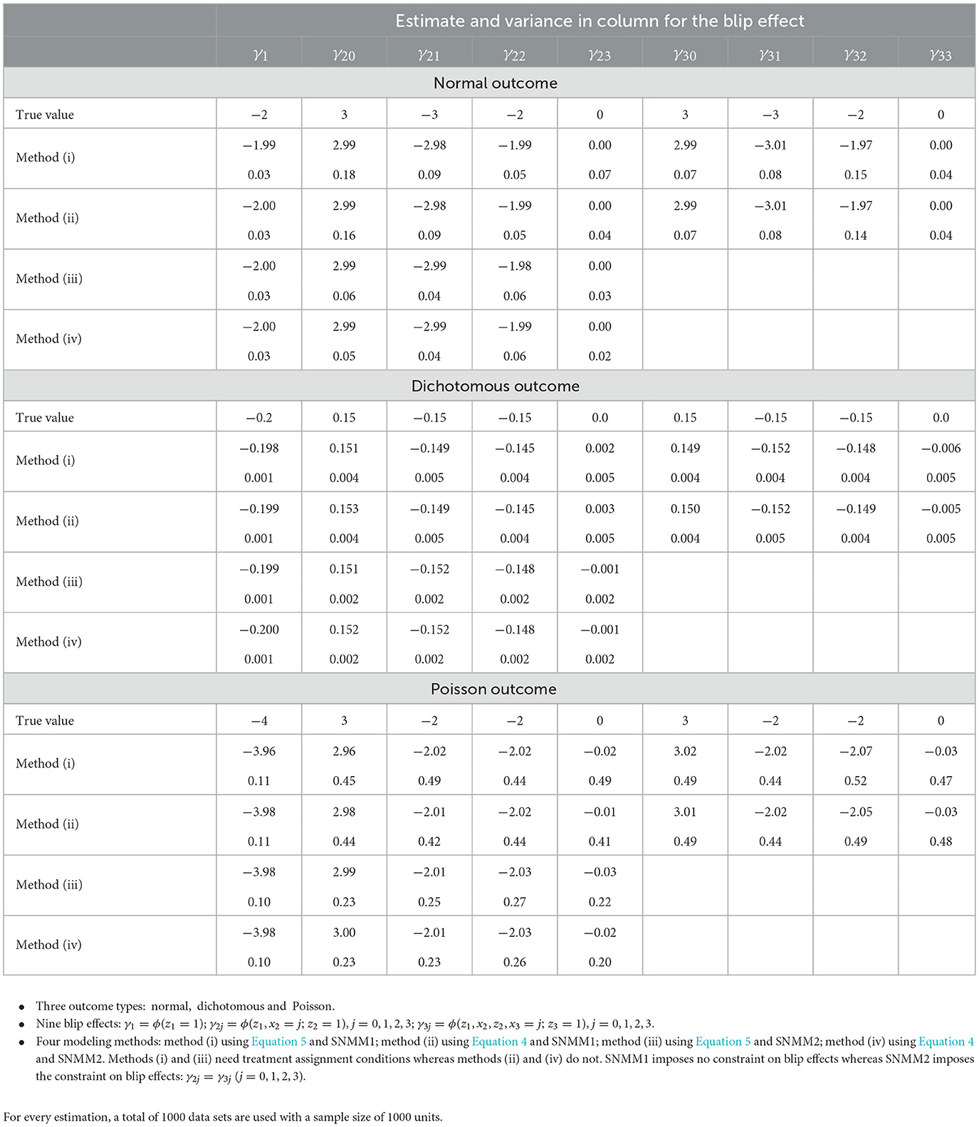
Table 1a. Estimate and variance of the blip effect obtained in Section 4 with our methods.

From Table 1b, the following observations can be made for estimating and testing the blip effects. First, all four methods achieve unbiased estimates and the nominal level of the coverage probability. Second, as compared to methods (i) and (ii) with SNMM1, methods (iii) and (iv) may impose SNMM2 across times t = 2, 3, reducing the number of blip effects and thus resulting in a smaller variance and a greater power for estimating and testing the blip effects. Third, methods (ii) and (iv) are based on Equation 4 and achieve nearly the same results as methods (i) and (iii) based on Equation 5, demonstrating that our method performs equally well with or without treatment assignment condition.

Table 1b

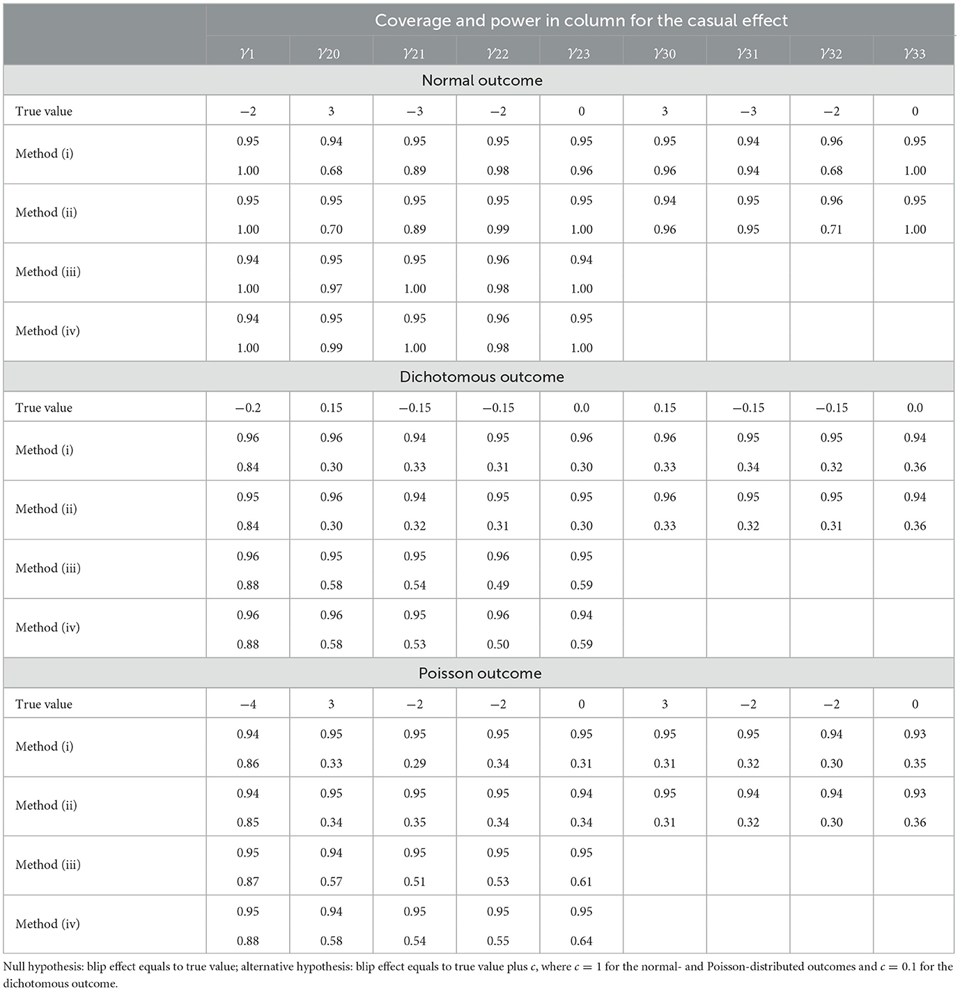
Table 1b. Wald test on the blip effect at the 0.05 significance level: coverage probability of 95 % confidence interval (coverage) and power of the test (power).

4.2 Comparison of our method with available methods

As described above, our method (iv) uses SNMM2 and Equation 4 when estimating and testing the blip effect without any treatment assignment conditions. Here, we compare this method with the following three available methods in the literature. Method (v) is the parametric method based on the well-known G-formula expressing the blip effect in terms of the standard parameters [5, 7]. Method (vi) is the marginal structural model based on the inverse probability of treatment weighting [5, 9]. Method (vii) is the G-estimation based on SNMM1 [1, 5, 11, 12]. These methods are reviewed in the introduction and also described in the context of the simulation in the Supplementary material.

With methods (iv)–(vii), we obtain the estimate and variance for the blip effect as well as the coverage probability and power for the hypothesis testing of the blip effect. The result is presented in Table 2. As seen from Table 2, all four methods achieve unbiased estimates and the nominal level of the coverage probability. Our method (iv) achieves the smallest variance and largest power due to SNMM2. Methods (v) and (vi) yield sizable variances and low powers due to the difficulty of imposing any SNMMs. Method (vii) yields a smaller variance and a larger power than methods (v) and (vi) due to SNMM1, but a larger variance and smaller power than method (iv) due to the difficulty of imposing SNMM2. In general, it is difficult to introduce SNMMs across different times with the G-estimation.

Table 2

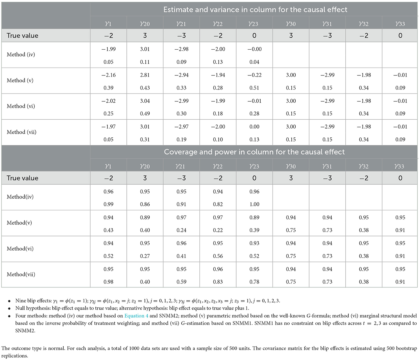
Table 2. Comparison of our method with available methods in Section 4: estimate and variance for the blip effect; Wald test on the blip effect at the 0.05 significance level: coverage probability of 95 % confidence interval (coverage) and power of the test (power).

It is also interesting to compare our method (iv) with method (vii) in terms of other modeling conditions than SNMM. With method (iv), we only need models for the point effects, which in this simulation are the three models for μ(z₁), μ(z₁, x₂, z₂), and μ(z₁, x₂, z₂, x₃, z₃) plus SNMM2. Standardization does not need additional models. With method (vii), we need the following models. First, a model for μ(x₃, z₃), which is smaller than μ(z₁, x₂, z₂, x₃, z₃) due to the treatment assignment condition. Second, a model for the baseline E{Y(D₂ = 0, D₃ = 0)∣x₂} together with SNMM1 at t = 2. Third, a model for baseline E{Y(D₁ = 0, D₂ = 0, D₃ = 0) together with SNMM1 at t = 1. In general, the baseline $E\left\{Y({\text{D}}_t^T=0)\mid {\text{h}}_t\right\}$ with the G-estimation is typically subject to model misspecification in comparison to the baseline E(Y∣h_t, z_t = 0) with our method; for this reason, the doubly robust version of the G-estimation may be used [5, 12]. Although it is not needed in the simple setting of this article, we may have a doubly robust version of our method by obtaining the doubly robust estimates for the point effects.

5 Influence of early diagnosis on cancer survival

5.1 Data and the identifying condition

In Sweden, patients usually seek medical help at hospitals near their residential areas. When cancer is diagnosed, they may stay at the diagnosing hospital or transfer to another hospital for treatment. The hospital that diagnoses cancer is called the diagnosing hospital, while the one that treats cancer is called the treating hospital. To evaluate the performance of diagnosing and treating hospitals, one may study the blip effects of diagnosing and treating hospitals among cancer patients after adjusting for patients' differences.

The data used in this study contain the information on 1, 070 stomach cancer patients from a clinical study during the period between 1988 and 1995 in hospitals located in central and northern Sweden [18]. Stomach cancer is highly malignant with a poor prognosis, so the 1-year survival is a good measure of the performance of both diagnosing and treating hospitals. A question of medical relevance is which types of diagnosing and treating hospitals, large vs. small, perform better on cancer outcomes, where the large type refers to the regional or county hospitals and the small type to local hospitals. One concern is that young patients diagnosed at local hospitals tend to have poor prognoses. This phenomenon is known as doctors' delay in the area of cancer diagnosis, but little studied statistically [19].

The diagnosing hospital is the treatment variable Z₁ at time t = 1: z₁ = 0 for small type and z₁ = 1 for large type. The treating hospital is the treatment variable Z₂ at t = 2: z₂ = 0 for small type and z₂ = 1 for large type. The outcome of interest is Y: y = 1 for a successful 1-year survival and y = 0 otherwise. The stationary covariates X₁ = (X₁₁, X₁₂, X₁₃) before Z₁ were measured with gender X₁₁, geographic area X₁₂ and age X₁₃. Gender was x₁₁ = 0 for female and x₁₁ = 1 for male. Geographic area was categorized into rural x₁₂ = 0 vs. urban x₁₂ = 1. Age took continuous values x₁₃. The time-dependent covariate between Z₁ and Z₂ was cancer stage X₂, taking the values x₂ = 1, 2, 3, 4 for cancer stages. The descriptive statistics are given in Table 3. The data and code are given by Yin [17].

Table 3

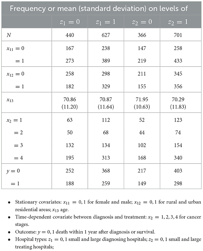
Table 3. Descriptive statistics for the data of 1067 patients in Section 5: frequencies or means (standard deviations) of covariates and outcome across the diagnosing and treating hospitals.

Notably, the data are unbalanced between diagnosing and treating hospitals: 981 patients did not transfer, 80 of them from small diagnosing hospitals to large ones, and only 6 from large to small diagnosing hospitals. According to Swedish medical experts, it was a typical transferal pattern. The small sample size and unbalanced data contribute to the small significance of our results. The confounding situation is described below.

Due to the long-term social welfare system and the relatively uniform culture in Sweden, most of the stationary covariates, such as education and socioeconomic status, have similar distributions across different hospitals and thus do not confound the blip effect. As a common practice in many epidemiological research studies in Sweden, the assumption of no unmeasured confounders is approximately satisfied for diagnosing hospital Z₁, at least after conditioning on gender x₁₁, residential area x₁₂, and age x₁₃. Similarly, the assumption of no unmeasured confounders is also approximately satisfied for treating hospital Z₂ conditional on the cancer stage x₂ and the diagnosing hospital z₁ in addition to (x₁₁, x₁₂, x₁₃). The causal DAG for diagnosing and treating hospital types is given in Figure 1.

Figure 1

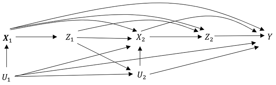
Figure 1. Causal DAG for diagnosing and treating hospital types in the medical examples of Section 5. Exposure: Z₁ for diagnosing hospital and Z₂ for treating hospitals. Stationary covariates: X₁ = X₁₁, X₁₂, X₁₃ for gender, residential area, and age. Time-dependent covariates between Z₁ and Z₂: X₂ for four cancer stages. Outcome: Y for one-year survival. Unmeasured covariates: U₁ unmeasured covariates before Z₁ and U₂ unmeasured covariates before Z₂. Neither confounds Z₁ and Z₂. This observational study mimics sequential randomized trial. Notably, diagnosing hospital Z₁ does not have direct influence on outcome Y as indicated by the missing arrow from Z₁ to outcome Y.

Without further examining the validity of the identifying condition, we will focus on the inference part of the medical example; interested readers may find a large body of literature on sensitivity analysis of the causal effect to the identifying condition (e.g., [20, 21]).

5.2 Estimating the standardized point effects

Because we aim at the effect modification of the blip effect by age, we divide the population at t = 1 into two strata U and L, where S₁ = U is the one with age x₁₃ smaller than the median and S₁ = L with age x₁₃ larger than or equal to the median. So, we have two standardized point effects Θ(S₁; z₁ = 1).

A large variety of methods are available for estimating the point effect in the framework of causal inference for single-point treatments (e.g., [5, 13–15]). As an illustration, we use the usual regression to estimate the point effects of diagnosing hospital z₁. Because the sample is small and only three stationary covariates—that is, x₁₁, x₁₂, x₁₃—are involved in the estimation, we model the conditional mean μ(x₁₁, x₁₂, x₁₃, z₁) = E(Y∣x₁₁, x₁₂, x₁₃, z₁) in the whole data set. For the sake of presentation, we use the linear model to estimate the point effect. Notably, we may use the logistic model, which only improves the estimation slightly.

We exclude the residential area x₁₂ at a significance level of 0.05, consistent with medical observations indicating that the residential area is less influential than gender and age. Finally, we obtain the regression model,

$\begin{array}{ll}\mu (x_{11},x_{13},z_1)={\beta }_1+x_{11}{\beta }_2+x_{13}{\beta }_3+z_1{\theta }_1.& (6)\end{array}$

From this model, we obtain the point effects of z₁ = 1 in stratum (x₁₁, x₁₃),

$\theta (x_{11},x_{13};z_1=1)=\mu (x_{11},x_{13},z_1=1)-\mu (x_{11},x_{13},z_1=0)={\theta }_1,$

which is the same for all (x₁₁, x₁₃). The standardized point effects are obtained by Θ(S₁; z₁ = 1) = E{θ(x₁₁, x₁₃; z₁ = 1)∣S₁} with respect to P(X₁₁ = x₁₁, X₁₃ = x₁₃∣S₁), where the point effect is estimated above while the probability is estimated by the corresponding proportion. Clearly, Θ(S₁; z₁ = 1) = θ₁ from Model 8. Therefore, we have the estimate $\hat{\Theta }(S_1;z_1=1)={\widehat{\theta }}_1$, but the variance of $\hat{\Theta }(S_1;z_1=1)$ is obtained by adjusting the variance of ${\widehat{\theta }}_1$ to the size of sub sample S₁.

To estimate the point effects of treating hospital z₂, we model the mean μ(x₁₁, x₁₂, x₁₃, z₁, x₂, z₂). We exclude x₁₂ at the significance level of 0.05. Furthermore, age x₁₃ has rather different influences on cancer survival for different cancer stages x₂, so we model the conditional mean separately for different x₂. Finally, we obtain the regression model,

$\begin{array}{ll}\{\begin{array}{l}\mu (x_{11},x_{13},x_2=1,z_2)={\beta }_4+x_{11}{\beta }_5+x_{13}{\beta }_6+z_2{\theta }_{21,0}+z_2{x}_{13}{\theta }_{21,3}\\ \mu (x_2=j,z_2)={\beta }_{7j}+z_2{\theta }_{2j},j=2,3,4\end{array}& (7)\end{array}$

From this model, we obtain the point effects of z₂ = 1 in stratum (x₁₁, x₁₃, x₂) for early cancer stage x₂ = 1,

$\begin{array}{l}\begin{array}{l}\theta (x_{11},x_{13},x_2=1;z_2=1)\\ =\mu (x_{11},x_{13},x_2=1,z_2=1)-\mu (x_{11},x_{13},x_2=1,z_2=0)\\ ={\theta }_{21,0}+x_{13}{\theta }_{21,3}.\end{array}\end{array}$

Averaging it with respect to P(X₁₁ = x₁₁, X₁₃ = x₁₃∣x₂ = 1),we obtain the average point effect of z₂ = 1 in stratum x₂ = 1,

${\theta }_{21}={\theta }_{21,0}+E(X_{13}\mid x_2=1){\theta }_{21,3}.$

In cancer stage x₂ = j = 2, 3, 4, we have,

$\theta (x_2=j;z_1=1)=\mu (x_2=j,z_1=1)-\mu (x_2=j,z_1=0)={\theta }_{2j}.$

Because the point effects are equal to the blip effects for the last treatment z₂ = 1, we use the point effects of z₂ = 1 as a special case of the standardized point effects in estimating and testing the blip effects of z₁ = 1 and z₂ = 1.

As seen from Models 8 and 9, residential area x₁₂ does not appear in μ(x₁₁, x₁₃, z₁) and μ(x₁₁, x₁₃, x₂, z₂) and thus are irrelevant to the standardized point effects and the blip effects of treatments. Hence, we remove x₁₂ from the following development.

5.3 Estimating and testing the blip effects

The point effect of diagnosing hospital results from both diagnosing and treating hospitals and thus cannot be used to evaluate the diagnosing hospital. In comparison, the blip effect of the diagnosing hospital represents the causal effect of the diagnosing hospital, while setting the treating hospitals as small ones, and thus can be used for evaluation.

To study the phenomenon of doctors' delay in cancer diagnosis [19], we suppose that the blip effect of large diagnosing hospital ϕ(x₁₁, x₁₃; z₁ = 1) is a linear function of age x₁₃, that is, age modifies the blip effect. Furthermore, because Z₂ is the last treatment variable in the treatment sequence, the blip effect of z₂ is equal to the point effect of z₂ as obtained from Model 9. Summarizing these observations, we specify an SNMM of the following form,

$\begin{array}{ll}\{\begin{array}{l}\varphi (x_{11},x_{13};z_1)={\gamma }_{1,0}{z}_1+{\gamma }_{1,3}{x}_{13}{z}_1\\ \varphi (x_{11},x_{13},z_1,x_2=1;z_2)={\gamma }_{21,0}{z}_2+{\gamma }_{21,3}{x}_{13}{z}_2\\ \varphi (x_{11},x_{13},z_1,x_2=j;z_2)={\gamma }_{2j}{z}_2,j=2,3,4.\end{array}& (8)\end{array}$

Thus, SNMM 8 is indexed by γ = (γ_{1, 0}, γ_{1, 3}, γ_{21, 0}, γ_{21, 3}, γ₂₂, γ₂₃, γ₂₄). Let γ₁ = E{ϕ(x₁₁, x₁₃; z₁ = 1)} be the blip effect of a large diagnosing hospital z₁ = 1 in the whole population. Then we have γ₁ = γ_{1, 0} + E(X₁₃)γ_{1, 3}, so γ_{1, 3} is the modification of the blip effect γ₁ by age. Let γ₂₁ = E{ϕ(x₁₁, x₁₃, z₁, x₂; z₂ = 1)∣x₂ = 1} be the blip effect of large treating hospital z₂ = 1 in low cancer stage x₂ = 1. Then we have γ₂₁ = γ_{21, 0} + E(X₁₃∣x₂ = 1)γ_{21, 3}, so γ_{21, 3} is the modification of the blip effect γ₂₁ by age in low cancer stage x₂ = 1. The blip effect of z₂ = 1 in cancer stage x₂ = j = 2, 3, 4 is γ_2j.

Because the blip effect ϕ(x₁₁, x₁₃; z₁ = 1) is indexed by two parameters γ_{1, 0} and γ_{1, 3} under SNMM, as expressed in Equation 8, we need two standardized point effects Θ(S₁; z₁ = 1) = E{θ(x₁₁, x₁₃; z₁ = 1)∣S₁} with respect to P(X₁₁ = x₁₁, X₁₃ = x₁₃∣S₁) for S₁ = U, L, as described and estimated in Section 5.2. Now by applying Equation 2 or Equation 4 to Θ(S₁; z₁ = 1), we obtain

$\begin{array}{l}\Theta (S_1;z_1=1)=E\{\varphi (x_{11},x_{13};z_1=1)\mid S_1\}+E\{\varphi (x_{11},x_{13},z_1=1,\hfill \\ x_2;z_2)\mid S_1,z_1=1\}-E\{\varphi (x_{11},x_{13},z_1=0,x_2;z_2)\mid S_1,z_1=0\}.\hfill \end{array}$

Here the first expectation is with respect to the P(X₁₁ = x₁₁, X₁₃ = x₁₃∣S₁), so we have

$E\left\{\varphi (x_{11},x_{13};z_1=1)\mid S_1\right\}={\gamma }_{1,0}+{\gamma }_{1,3}E(x_{13}\mid S_1).$

The second expectation is with respect to P(X₂ = x₂, Z₂ = z₂∣x₁₁, x₁₃, z₁ = 1) P(X₁₁ = x₁₁, X₁₃ = x₁₃∣S₁) and the third one to P(X₂ = x₂, Z₂ = z₂∣x₁₁, x₁₃, z₁ = 0) P(X₁₁ = x₁₁, X₁₃ = x₁₃∣S₁). By using ϕ(x₁₁, x₁₃, z₁, x₂; z₂ = 0) = 0, the second and third expectations are, for z₁ = 1, 0,

$\begin{array}{l}E\{\varphi (x_{11},x_{13},z_1,x_2;z_2)\mid S_1,z_1\}=\hfill \\ {\displaystyle {\sum }_{j=1,2,3,4}E\{\varphi (x_{11},x_{13},z_1,x_2=j;z_2=1)}\hfill \\ \text{P}(x_2=j,z_2=1\mid x_{11},x_{13},z_1)\mid S_1\}\hfill \end{array}$

with respect to P(X₁₁ = x₁₁, X₁₃ = x₁₃∣S₁). Now by inserting SNMM, as provided in Equation 8, we obtain

$\begin{array}{l}E\{\varphi (x_{11},x_{13},z_1,x_2;z_2)\mid S_1,z_1\}={\gamma }_{21,3}E\{x_{13}P(x_2=1,z_2=1\mid \hfill \\ x_{11},x_{13},z_1)\mid S_1\}\hfill \\ +{\gamma }_{21,0}E\{P(x_2=1,z_2=1\mid x_{11},x_{13},z_1)\mid S_1\}\hfill \\ +{\displaystyle {\sum }_{j=2}^4{\gamma }_{2j}E\{P(x_2=j,z_2=1\mid x_{11},x_{13},z_1)\mid S_1\}.}\hfill \end{array}$

Let A = E(x₁₃∣S₁). Let B and C_j (j = 1, 2, 3, 4) be the mean differences,

$\begin{array}{l}\begin{array}{l}B=E\left\{x_{13}P(x_2=1,z_2=1\mid x_{11},x_{13},z_1=1)\mid S_1\right\}-\\ E\left\{x_{13}P(x_2=1,z_2=1\mid x_{11},x_{13},z_1=0)\mid S_1\right\};\\ C_j=E\left\{P(x_2=j,z_2=1\mid x_{11},x_{13},z_1=1)\mid S_1\right\}-\\ E\left\{P(x_2=j,z_2=1\mid x_{11},x_{13},z_1=0)\mid S_1\right\}.\end{array}\end{array}$

Then we have

$\begin{array}{l}\Theta (S_1;z_1=1)={\gamma }_{1,0}+{\gamma }_{1,3}A+{\gamma }_{21,3}B+{\gamma }_{21,0}{C}_1+{\displaystyle {\sum }_{j=2,3,4}}{\gamma }_{2j}{C}_j,\\ S_1=U,L& (9)\end{array}$

Using the observed proportions $\hat{P}(x_2,z_2\mid x_{11},x_{13},z_1)$ and $\hat{P}(x_{11},x_{13}\mid S_1)$, we obtain the estimates $\hat{A}$, $\hat{B}$, and ${\hat{C}}_j$ without modeling.

Now we consider the blip effect of treating hospital z₂. It is equal to the point effect of z₂, because Z₂ is the last treatment variable in the treatment sequence. Thus, from Model 9 in Section 5.2 and SNMM 11, we obtain

$\begin{array}{ll}{\theta }_{21,0}={\gamma }_{21,0},{\theta }_{21,3}={\gamma }_{21,3},{\theta }_{2j}={\gamma }_{2j}j=2,3,4.& (10)\end{array}$

The estimates of θ_{21, 0}, θ_{21, 3} and θ_2j are obtained from Section 5.2. Now, conditional on all covariates and treatments {x₁₁, x₁₃, z₁, x₂, z₂}, we use Equations 9 and 10 together as a regression model to estimate γ, where the response variables are $\hat{\Theta }(S_1;z_1=1)={\widehat{\theta }}_1$, ${\widehat{\theta }}_{21,0}$, ${\widehat{\theta }}_{21,3}$ and ${\widehat{\theta }}_{2j}$; the explanatory variables are $\hat{A}$, $\hat{B}$, ${\hat{C}}_j$ and one. The bootstrap method is used to obtain the covariance matrix $\text{cov}(\hat{\gamma })$ incorporating the variability of all treatments and covariates. With $\hat{\gamma }$ and $\text{cov}(\hat{\gamma })$, we conduct the hypothesis testing on γ. The result is presented in Table 4. For the sake of comparison, we also present the results for the point effects of z₁ = 1 and z₂ = 1.

Table 4

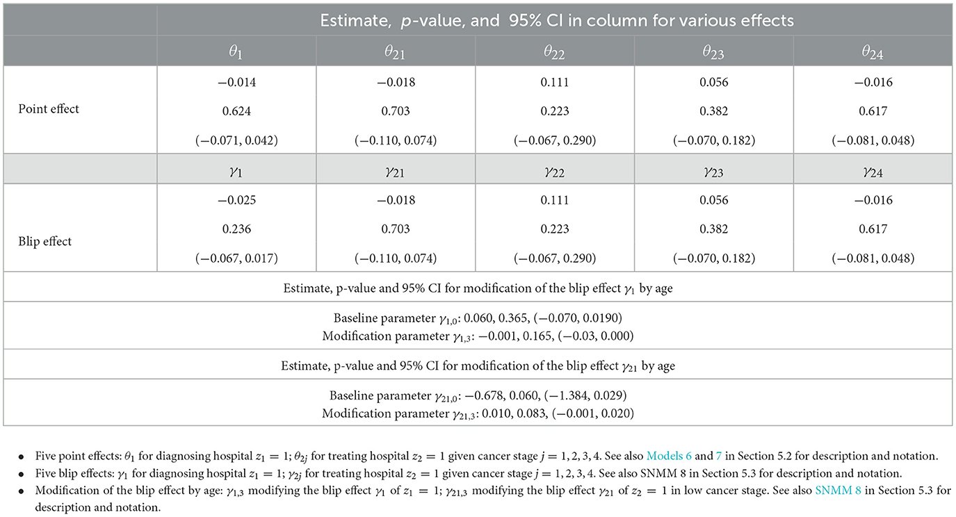
Table 4. Point effects and blip effects of diagnosing and treating hospitals on 1-year cancer survival in Section 5: estimate, p-value and 95 % CI.

5.4 Causal analysis of blip effects based on Table 4

From Table 4, we see that the point effect of a large treating hospital z₂ = 1 is equal to the blip effect of z₂ = 1, that is, θ_2j = γ_2j in cancer stage x₂ = j (j = 1, 2, 3, 4). We also see that the point effect of a large diagnosing hospital z₁ = 1 is not equal to the blip effect of z₁ = 1, that is, θ₁ ≠ γ₁.

The following observations are medically interesting. First, patients with the moderate cancer stage x₂ = 2, 3 benefit from large treating hospitals z₂ = 1 as seen from ${\widehat{\gamma }}_{22}=0.111$ (p-value = 0.223) and ${\widehat{\gamma }}_{23}=0.056$ (p-value = 0.382), despite somewhat small significance. The possible reason is due to the skillful medical workers and good facilities at these hospitals. Second, patients with the advanced cancer stage x₂ = 4 benefit slightly from small treating hospitals z₂ = 0 as seen from ${\widehat{\gamma }}_{24}=-0.016<0$ (p-value = 0.617), possibly due to good care at these hospitals, despite small significance. Third, for the low cancer stage x₂ = 1, there is a modification of the blip effect of a large treating hospital z₁ = 1 by age x₁₃, as seen from ${\widehat{\gamma }}_{21,3}=0.010$ per year (p-value = 0.083). Because $\widehat{\varphi }(x_{11},x_{13},z_1,x_2=1;z_2=1)={\widehat{\gamma }}_{21,0}+x_{13}{\widehat{\gamma }}_{21,3}=-0.678+0.010x_{13}>0$ for x₁₃>68, patients of age >68 benefit from large treating hospitals z₂ = 1. This observation reflects the fact that old patients usually have more comorbidities, and large hospitals are probably better at dealing with comorbidities.

Fourth, patients benefit overall from small diagnosing hospitals z₁ = 0 as seen from ${\widehat{\gamma }}_1=-0.025$ (p-value = 0.236). However, there is a modification of the blip effect of a large diagnosing hospital z₁ = 1 by age x₁₃, as seen from ${\widehat{\gamma }}_{1,3}=-0.001$ per year (p-value = 0.165). Because $\widehat{\varphi }(x_{11},x_{13};z_1=1)={\widehat{\gamma }}_{1,0}+x_{13}{\widehat{\gamma }}_{1,3}=0.060-0.001x_{13}>0$ for x₁₃ < 60, patients of age < 60 benefit from large diagnosing hospital z₁ = 1. This reflects the delay in diagnosing stomach cancer among young patients at small diagnosing hospitals, where cancer in young patients is rare (phenomenon of doctors' delay).

To summarize the key medical findings from this analysis, large and small hospitals differ in diagnosing stomach cancer. Small hospitals demonstrate greater effectiveness in detecting early-stage cases due to shorter examination wait times. However, they need to pay closer attention to younger patients, who are often underrecognized in smaller facilities.

6 Conclusion

In many practices, a single-point treatment often fails to achieve the desired outcome. More often, a sequence of treatments is implemented, where a new situation often arises from the early treatments and also influences the assignment of subsequent treatments. Under such circumstances, designing and conducting sequential randomized trials is significantly more challenging than conducting randomized trials for single-point treatments. Consequently, data arising from a sequence of treatments are often observational, where treatment assignments are unknown.

The blip effect is such a parameter that involves all steps of the complex stochastic process, making it highly challenging to estimate and test in a single step with a single model without bias and loss of efficiency. In this article, we estimate and test the blip effects of treatments in sequence via the standardized point effects of treatments without requiring treatment assignment conditions. As described in Sections 2 and 3, our method is implemented in three steps. First, we choose strata reflective of our scientific interest in the blip effects. Second, we estimate the point effects using available methods within the framework of causal inference for single-point treatments, and then standardize these estimated point effects in strata to reduce their dimensionality. Finally, we use the estimated standardized point effects to estimate and test the blip effects by the usual regression. These steps are familiar to applied statisticians.

Our method resembles the G-estimation, both using SNMMs and the identifying condition [1, 5, 11, 12]. Two comments are given comparing the two methods. First, as described in Sections 2.3 and 3 and demonstrated by simulations in Section 4, our method places emphasis on different aspects, that is, the pattern of blip effects over time and a targeted analysis of blip effects. Second, both methods require a strong identifying condition for all blip effects in the population. The requirement is the major limitation for using the two methods in many realistic problems. In contrast, due to the targeted analysis, our parameters of interest are fewer than those with the G-estimation. We conjecture that our method should be more robust to the identifying condition. However, the simulation and real example in this article do not permit a thorough evaluation of the usefulness of these properties in addressing complex problems under varying assumptions in comparison to available methods such as the G-estimation. Therefore, comprehensive simulation studies and real-world examples are needed to explore more realistic scenarios and challenges in further development of this article.

Data availability statement

The datasets presented in this study can be found in online repositories. The names of the repository/repositories and accession number(s) can be found below: Zenodo, https://doi.org/10.5281/zenodo.7614934.

Ethics statement

The studies involving humans were approved by the Ethical Committee approval (DNR880113/13, x121) from the ethical review board of Uppsala University. The studies were conducted in accordance with the local legislation and institutional requirements. The participants provided their written informed consent to participate in this study.

Author contributions

YaL: Writing – review & editing, Writing – original draft. YiL: Validation, Conceptualization, Writing – review & editing, Methodology. LY: Resources, Software, Methodology, Conceptualization, Writing – review & editing. XW: Conceptualization, Supervision, Funding acquisition, Writing – review & editing, Methodology, Writing – original draft, Validation.

Funding

The author(s) declare that financial support was received for the research and/or publication of this article. Wang declares partial financial support by the Swedish Research Council with the grant number 2019-02913.

Acknowledgments

All authors are grateful to the reviewers for their comments and advice, which have improved the article considerably.

Conflict of interest

The authors declare that the research was conducted in the absence of any commercial or financial relationships that could be construed as a potential conflict of interest.

Generative AI statement

The author(s) declare that no Gen AI was used in the creation of this manuscript.

Any alternative text (alt text) provided alongside figures in this article has been generated by Frontiers with the support of artificial intelligence and reasonable efforts have been made to ensure accuracy, including review by the authors wherever possible. If you identify any issues, please contact us.

Publisher's note

All claims expressed in this article are solely those of the authors and do not necessarily represent those of their affiliated organizations, or those of the publisher, the editors and the reviewers. Any product that may be evaluated in this article, or claim that may be made by its manufacturer, is not guaranteed or endorsed by the publisher.

Supplementary material

The Supplementary Material for this article can be found online at: https://www.frontiersin.org/articles/10.3389/fams.2025.1650059/full#supplementary-material

References

1. Robins JM. Causal Inference from complex longitudinal data. In:Berkane M, , editor. Latent Variable Modeling and Applications to Causality, Lecture Notes in Statistics. New York: Springer-Verlag (1997). p. 69–117.

Google Scholar

2. Wang X, Yin, L. Identifying and estimating net effects of treatments in sequential causal inference. Elect J Statist. (2015) 9:1608–43. doi: 10.1214/15-EJS1046

Crossref Full Text | Google Scholar

3. Almirall D, Have TT, Murphy SA. Structural nested mean models for assessing time-varying effect moderation. Biometrics. (2010) 66:131–9. doi: 10.1111/j.1541-0420.2009.01238.x

PubMed Abstract | Crossref Full Text | Google Scholar

4. Boruvka A, Almirall D, Witkiewitz K, Murphy SA. Assessing time-varying causal effect moderation in mobile health. J Am Stat Assoc. (2018) 113:1112–11121. doi: 10.1080/01621459.2017.1305274

PubMed Abstract | Crossref Full Text | Google Scholar

5. Hernan MA, Robins JM. Causal Inference. Boca Raton: CRC Press. (2020).

Google Scholar

6. Robins JM. A new approach to causal inference in mortality studies with sustained exposure periods - application to control of the healthy worker survival effect. Mathemat Model. (1986) 7:1393–512. doi: 10.1016/0270-0255(86)90088-6

Crossref Full Text | Google Scholar

7. Taubman SL, Robins JM, Mittleman MA, Hernán MA. Intervening on risk factors for coronary heart disease: an application of the parametric G-formula. Int J Epidemiol. (2009) 38:1599–611. doi: 10.1093/ije/dyp192

PubMed Abstract | Crossref Full Text | Google Scholar

8. Henderson R, Ansell P, Alshibani D. Regret-regression for optimal dynamic treatment regimes. Biometrics. (2010) 66:1192–201. doi: 10.1111/j.1541-0420.2009.01368.x

PubMed Abstract | Crossref Full Text | Google Scholar

9. Robins JM. Association, causation, and marginal structural models. Synthese. (1999) 121:151–79. doi: 10.1023/A:1005285815569

Crossref Full Text | Google Scholar

10. Pan Y, Zhao YQ. Improved doubly robust estimation in learning optimal individualized treatment rules. J Am Statist Assoc. (2021) 116:283–94. doi: 10.1080/01621459.2020.1725522

PubMed Abstract | Crossref Full Text | Google Scholar

11. Vansteelandt S, Joffe M. Structural nested models and g-estimation: the partially realized promise. Statist Sci. (2014) 29:707–31 doi: 10.1214/14-STS493

Crossref Full Text | Google Scholar

12. Wallace MP, Moodie EEM. Doubly-robust dynamic treatment regimen estimation via weighted least squares. Biometrics. (2015) 71:636–44. doi: 10.1111/biom.12306

PubMed Abstract | Crossref Full Text | Google Scholar

13. Rosenbaum PR, Rubin DB. The central role of the propensity score in observational studies for causal effects. Biometrika. (1983) 70:41–55. doi: 10.1093/biomet/70.1.41

Crossref Full Text | Google Scholar

14. van der Laan, M. Targeted maximum likelihood based causal inference: part I. Int J Biostatist. (2010a) 6:2. doi: 10.2202/1557-4679.1211

PubMed Abstract | Crossref Full Text | Google Scholar

15. van der Laan M. Targeted maximum likelihood based causal inference: part II. Int J Biostatist. (2010b) 6:3. doi: 10.2202/1557-4679.1241

PubMed Abstract | Crossref Full Text | Google Scholar

16. Wang X, Yin L. G-formula for the sequential causal effect and blip effect of treatment in sequential causal inference. Ann Stat. (2020) 48:138–60. doi: 10.1214/18-AOS1795

Crossref Full Text | Google Scholar

17. Yin L. Data and Code for Statistical Modelling in Sequential Causal Inference. Zenodo. (2023). doi: 10.5281/zenodo.7614934

Crossref Full Text | Google Scholar

18. Hansson LE, et al. Surgery for stomach cancer in a defined Swedish population: current practices and operative results. Swedish gastric cancer study group. Eur J Surg. (2000) 166:787–975. doi: 10.1080/110241500447425

PubMed Abstract | Crossref Full Text | Google Scholar

19. Round T, Steed L, Shankleman J, Bourke L, Risi L. Primary care delays in diagnosing cancer: what is causing them and what can we do about them? J Royal Soc Med. (2013) 106:437–40. doi: 10.1177/0141076813504744

PubMed Abstract | Crossref Full Text | Google Scholar

20. Ding P, VanderWeele TJ. Sensitivity analysis without assumptions. Epidemiology. (2016) 27:368–77. doi: 10.1097/EDE.0000000000000457

PubMed Abstract | Crossref Full Text | Google Scholar

21. Rosenbaum PR. Design sensitivity in observational studies. Biometrika. (2004) 91:153–64. doi: 10.1093/biomet/91.1.153

Crossref Full Text | Google Scholar

22. Chakraborty B, Murphy SA. Dynamic treatment regimes. Ann Rev Statist Appl. (2014) 1:447–64. doi: 10.1146/annurev-statistics-022513-115553

PubMed Abstract | Crossref Full Text | Google Scholar

Appendix

Proofs for Equations 2 and 3

Proof of Equation 2: Under the identifying condition, by applying Equation 17 in Theorem 2 of Wang and Yin [16] and using ϕ(h_t; z_t = 0) = 0, we obtain

$\begin{array}{r}\theta ({\text{h}}_t;z_t)=\varphi ({\text{h}}_t;z_t)+{\displaystyle \sum _{s=t+1}^T}E\left\{\varphi ({\text{h}}_s;z_s)\mid {\text{h}}_t,z_t\right\}\\ -{\displaystyle \sum _{s=t+1}^T}E\left\{\varphi ({\text{h}}_s;z_s)\mid {\text{h}}_t,0\right\}\end{array}$

where the first expectation is with respect to $\text{P}({\text{X}}_{t+1}^s,{\text{Z}}_{t+1}^{s-1},Z_s\mid {\text{h}}_t,z_t)$ and the second one to $\text{P}({\text{X}}_{t+1}^s,{\text{Z}}_{t+1}^{s-1},Z_s\mid {\text{h}}_t,0)$. This equation implies a rather intuitive observation, where the point effect is a sum of the blip effects of individual treatments in sequence on the outcome. Averaging the above equation with respect to P(H_t∣S_t), we obtain Equation 2.

Proof of Equation 3: We will prove that Equation 2 becomes Equation 3 under the assignment condition P(Z_t∣h_t) = P(Z_t∣S_t). The condition implies the probability equalities P(H_t∣S_t) = P(H_t∣S_t, z_t) = P(H_t∣S_t, 0), so we have

$E\left\{\mu ({\text{h}}_t,z_t)\mid S_t\right\}=E\left\{\mu ({\text{h}}_t,z_t)\mid S_t,z_t\right\}=\mu (S_t,z_t).$

In contrast, according to Equation 1 we have

$\Theta (S_t;z_t)=E\left\{\theta (S_t;z_t)\mid S_t\right\}=E\left\{\mu ({\text{h}}_t,z_t)\mid S_t\right\}-E\left\{\mu ({\text{h}}_t,0)\mid S_t\right\}.$

Thus, the left-hand side of Equation 2 becomes

$\Theta (S_t;z_t)=\mu (S_t,z_t)-\mu (S_t,0)=\theta (S_t;z_t),$

which is the left-hand side of Equation 3. With the above probability equalities, we have that the first expectation in the right-hand side of Equation 2 becomes

$E\left\{\varphi ({\text{h}}_t;z_t)\mid S_t\right\}=E\left\{\varphi ({\text{h}}_t;z_t)\mid S_t,z_t\right\},$

which is the first expectation in the right-hand side of Equation 3. Because of P(H_t∣S_t) = P(H_t∣S_t, z_t) = P(H_t, Z_t∣S_t, z_t), the probability in the second expectation of the right-hand side of Equation 2 is

$\begin{array}{l}\text{\hspace{0.17em}\hspace{0.17em}\hspace{0.17em}\hspace{0.17em}\hspace{0.17em}\hspace{0.17em}\hspace{0.17em}\hspace{0.17em}\hspace{0.17em}\hspace{0.17em}\hspace{0.17em}\hspace{0.17em}\hspace{0.17em}\hspace{0.17em}\hspace{0.17em}\hspace{0.17em}\hspace{0.17em}\hspace{0.17em}\hspace{0.17em}\hspace{0.17em}\hspace{0.17em}\hspace{0.17em}\hspace{0.17em}\hspace{0.17em}\hspace{0.17em}\hspace{0.17em}P}(X_{t+1}^s,Z_{t+1}^{s-1},Z_s\mid h_t,z_t)\text{P}(H_t\mid S_t)\\ =\text{P}(X_{t+1}^s,Z_{t+1}^{s-1},Z_s\mid h_t,z_t)\text{P}(H_t,Z_t\mid S_t,z_t)=\text{P}(H_t,Z_t,X_{t+1}^s,\\ Z_{t+1}^{s-1},Z_s\mid S_t,z_t).\end{array}$

Furthermore, because of ${\text{H}}_s=\{{\text{H}}_t,Z_t,{\text{X}}_{t+1}^s,{\text{Z}}_{t+1}^{s-1}\}$, we have

$\begin{array}{l}\text{P}({\text{H}}_t,Z_t,{\text{X}}_{t+1}^s,{\text{Z}}_{t+1}^{s-1},Z_s\mid S_t,z_t)=\text{P}({\text{H}}_s,Z_s\mid S_t,z_t).\end{array}$

Thus, the second expectation in the right-hand side of Equation 2 becomes the second expectation in the right-hand side of Equation 3. Similarly, we prove that the third expectation in the right-hand side of Equation 2 becomes the third one in the right-hand side of Equation 3. Therefore we have proved Equation 3.