Inference on the scale-inflated gamma distribution applied to Malaysian household income

Modeling income distributions is crucial for understanding inequality and providing evidence-based policy support. A key challenge, however, lies in evaluating the extent to which household income inflates over time. While income is inherently random, it exhibits a persistent upward trend, and fitting income distributions using conventional models often leads to inconsistent parameter estimates. This highlights the necessity of explicitly incorporating inflation-adjusted scaling to preserve proper statistical properties. To address this gap, we introduce the Scale-Inflated Gamma (SIG) distribution, which extends the standard Gamma distribution by including an inflation-adjusted scale parameter (δ), thereby providing greater flexibility in capturing heterogeneous income dynamics. Standard models such as the Lognormal, Pareto, or Generalized Beta of the Second Kind (GB2) systematically underestimate upper-tail incomes and fail to capture inflation-adjusted heterogeneity across subgroups (B40, M40, T20). The SIG model, in contrast, strikes a balance between parsimony and flexibility by directly adjusting for inflationary scale shifts. For instance, while the Gamma distribution underestimates the 95th percentile by 10%–12% in 2019, the SIG model reduces this bias to approximately 3%, accurately reflecting income dynamics across B40, M40, and T20 groups. We develop the theoretical foundations of the SIG distribution by deriving its probability density function (PDF), cumulative distribution function (CDF), and moments. Parameters are initially estimated using the method of moments and then refined through maximum likelihood estimation (MLE). To assess estimator precision, we derive the Fisher information matrix, using the inverse Hessian to approximate the variance–covariance matrix, thus ensuring reliable inference. A Monte Carlo simulation study is conducted to evaluate the consistency and efficiency of the estimators under various sample sizes. The SIG model is subsequently applied to Malaysian Household Income Survey (HIS) data spanning the period from 2007 to 2022. Results demonstrate that the SIG distribution offers a superior fit for modeling income inequality and upper-tail behavior compared to conventional models. Overall, the study establishes the SIG distribution as a theoretically robust and policy-relevant framework for analyzing income patterns in inflation-sensitive and structurally diverse economies.

1 Introduction

Rising income inequality has become a critical concern in Malaysia over the past two decades, particularly as disparities between the B40, M40, and T20 groups have widened [1, 4]. These disparities stem not only from structural economic changes but also from persistent inflation, which erodes purchasing power unevenly across income segments [5, 6]. Such dynamics underscore the necessity for statistical tools capable of accurately representing income distributions under inflationary pressures, especially to inform targeted policy interventions [3].

Classical income distribution models, such as the Lognormal and Gamma distributions, have long been favored for their tractability in estimation and interpretation [7, 8]. However, they systematically underestimate upper-tail incomes and fail to accommodate inflation-adjusted shifts in the distribution. More flexible models like GB2 address some of these limitations, yet they often introduce complexity that impedes interpretability in applied policy settings [9]. In light of these challenges, scale-augmented approaches that adjust for inflation and heterogeneity have garnered increasing attention [10, 11]. A critical gap remains in evaluating how much household income increases over time. Although income is inherently random, it exhibits a persistent upward trend, and fitting income using conventional distributions without explicitly incorporating inflationary effects often leads to inconsistent parameter estimates and biased statistical properties [1, 2].

This gap is especially evident in upper-tail modeling: while conventional models consistently underestimate high-income observations, particularly in the upper 95th percentile, the proposed SIG model captures these dynamics with substantially greater accuracy, thereby offering a more faithful representation of income inequality. To fill this gap, we propose the Scale-Inflated Gamma (SIG) distribution. By introducing an inflation-adjusted scale parameter (δ), SIG flexibly models upper-tail behavior while preserving the familiar shape properties of the Gamma distribution. Visual evidence, via boxplots and kernel density estimates, reveals progressively heavier upper tails in Malaysian household income distributions from 2007 to 2022 (Figures 1, 2), illustrating the inadequacy of conventional models under inflationary dynamics.

Figure 1

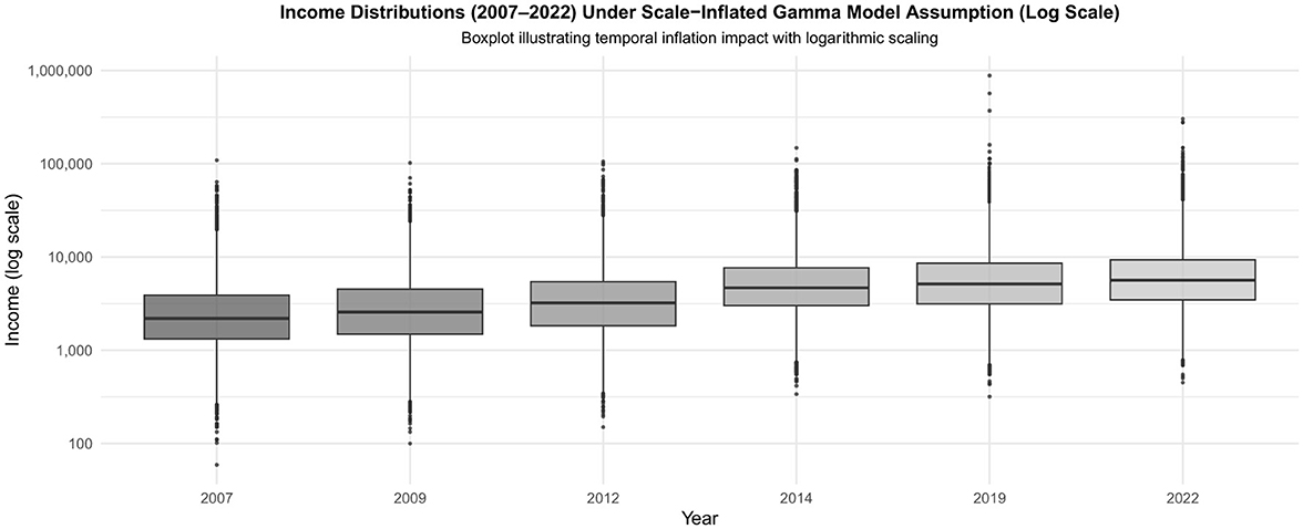
Figure 1. Boxplots of household income distributions across survey years (2007–2022) under logarithmic scaling. The presence of extreme outliers and heavy right tails underscores the inadequacy of conventional models and justifies the use of the Scale-Inflated Gamma (SIG) distribution, which better accommodates scale shifts and tail behavior.

Figure 2

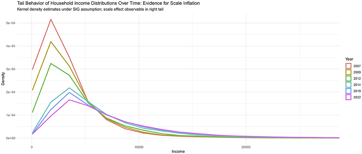
Figure 2. Kernel density estimates of household income distributions (2007–2022). The progressively heavier right tails over time highlight the necessity of models such as the SIG distribution, which incorporates a scale-inflation parameter to capture inflation-adjusted dynamics and upper-tail behavior.

This study applies the Scale-Inflated Gamma (SIG) distribution to Malaysian Household Income Survey (HIS) data from 2007 to 2022 to assess its performance relative to conventional alternatives. We estimate parameters via maximum likelihood estimation (MLE) and assess model fit using information criteria such as AIC and BIC. Additionally, we utilize visual tools (e.g., empirical cumulative distribution function plots, boxplots) and statistical diagnostics to validate the tail behavior modeling. The results position the SIG distribution as a theoretically grounded and practically relevant framework for analyzing income distributions under inflationary conditions, with implications for measuring inequality, monitoring subgroup dynamics, and informing policy design in Malaysia and similar economies.

In addition to the theoretical formulation, we conduct formal model comparisons using likelihood-based hypothesis testing and model selection metrics such as AIC and BIC. While our empirical focus centers on comparing the SIG model with the conventional Gamma distribution, we also situate our findings within the broader literature. Specifically, prior studies have shown that the Lognormal distribution tends to underestimate tail inequality [6], and the Pareto distribution is suited only for modeling the upper tail. It lacks inflation adjustment [4], and the GB2 distribution, though flexible, suffers from interpretability challenges in policy contexts [9]. Moreover, Yu et al. [12] highlight the advantages of using information criteria, such as AIC and BIC, for distributional comparison, which supports our evaluation framework. Collectively, our findings confirm that the SIG model offers a statistically robust and practically relevant alternative for modeling inflation-adjusted income dynamics and inequality.

2 General properties of the scale-inflated gamma distribution

This section formally introduces the Scale-Inflated Gamma (SIG) distribution by extending the conventional Gamma model to account for inflation-adjusted scaling across time. The SIG framework is governed by three primary parameters: the shape parameter α > 0, the baseline scale parameter θ > 0, and the scale-inflation parameter δ > − 1. The inflation-adjusted scale parameter is denoted by β = (1 + δ)^kθ, where k ∈ ℕ represents the number of time periods since the baseline. This formulation enables the model to dynamically adjust the scale of the income distribution over time, effectively capturing the erosion of purchasing power due to inflation. Each parameter plays a distinct role: α controls the skewness and dispersion of the distribution, θ anchors the scale in the base period, and δ modulates how the scale evolves. These structural components jointly enable the SIG distribution to model income dynamics under inflationary regimes with flexibility. The following subsections develop the full probabilistic specification of the model, including its probability density function (PDF), log-likelihood function, gradient vector, and Fisher Information Matrix.

Let X ~ F_X(α, β) be a random variable with mean 𝔼(X ∣ β) and variance Var(X ∣ β), where α > 0 and β > 0 denote the shape and scale parameters, respectively. These parameters can be written in vector form as ε = (α, β)′, where the prime symbol (′) denotes the transpose of a vector. Inflationary scaling is introduced through the transformation

$Y={(1+\delta )}^{k}X,\delta >-1,k\in \mathbb{N},$

where δ is the scale-inflation parameter and k is the number of periods. The extended parameter set is expressed as υ = (θ, δ)′, so that Y follows the scale-inflated distribution

$Y~F_Y(\alpha ,\theta ,\delta )\equiv F_X[\alpha ,\beta (\upsilon )],$

with β = (1 + δ)^kθ, and the complete parameter vector is denoted as λ = (α, θ, δ)′, where the prime symbol (′) indicates vector transposition.

Given the distribution functions of X, with cumulative distribution function (CDF) F_X(x; ε) and probability density function (PDF) f_X(x; ε), the corresponding functions for Y are written as

$F_Y(y;\alpha ,\theta ,\delta )\equiv F_Y[y;\alpha ,\beta (\upsilon )],f_Y(y;\alpha ,\theta ,\delta )\equiv f_Y[y;\alpha ,\beta (\upsilon )],$

$\text{ for }X>0,Y>0.$

For the log-PDF of X, denoted ln[f_X(x; ε)], the score functions (first derivatives) are defined as

$\begin{array}{ll}{g}_{{\epsilon }_i}(x)=\frac{\partial }{\partial {\epsilon }_i}ln{f}_X(x;\epsilon ).& (2.1)\end{array}$

For a complete random sample, the unbiasedness condition holds: 𝔼[g_εi(X)] = 0, which follows from standard likelihood theory [13].

The second derivatives (Hessian components) of the log-PDF of X are given by

$\begin{array}{ll}{h}_{{\epsilon }_i{\epsilon }_j}(x)=\frac{{\partial }^2}{\partial {\epsilon }_i\partial {\epsilon }_j}ln{f}_X(x;\epsilon ).& (2.2)\end{array}$

For the inflated variable Y, the log-PDF has derivatives

$\begin{array}{ll}{g}_{{\epsilon }_i}(y)=\frac{\partial }{\partial {\epsilon }_i}ln{f}_Y(y;\epsilon ),& (2.3)\end{array}$

and, defining $g_{\beta }(y)=\frac{\partial }{\partial \beta }ln{f}_Y(y;\epsilon )$, the score functions with respect to υ = (θ, δ)′ are

$\begin{array}{ll}{g}_{{\upsilon }_i}(y)=g_{\beta }(y)·\frac{\partial \beta }{\partial {\upsilon }_i}.& (2.4)\end{array}$

The corresponding Hessian terms are obtained as

$\begin{array}{ll}{h}_{{\epsilon }_i{\epsilon }_j}(y)=\frac{\partial }{\partial {\epsilon }_i}{g}_{{\epsilon }_j}(y),& (2.5)\end{array}$

and for υ = (θ, δ)′, where the prime symbol (′) denotes the transpose of a vector,

$\begin{array}{ll}{h}_{{\upsilon }_i{\upsilon }_j}(y)=h_{\beta \beta }(y)\frac{\partial \beta }{\partial {\upsilon }_i}\frac{\partial \beta }{\partial {\upsilon }_j}+h_{\beta }(y)\frac{{\partial }^2\beta }{\partial {\upsilon }_i\partial {\upsilon }_j}.& (2.6)\end{array}$

Finally, since the SIG distribution involves both the shape parameter α and the inflation parameters υ = (θ, δ)′, mixed derivatives are given by

$\begin{array}{ll}{h}_{\alpha {\upsilon }_i}(y)=h_{\alpha \beta }(y)\frac{\partial \beta }{\partial {\upsilon }_i}+h_{\beta }(y)\frac{{\partial }^2\beta }{\partial \alpha \partial {\upsilon }_i}.& (2.7)\end{array}$

Throughout this section, the symbols g_α, g_θ, g_δ are used to denote the score functions, i.e., the first-order derivatives of the log-likelihood, while h_αθ, h_θδ represent the corresponding Hessian components, i.e., the second-order derivatives. The sample sizes are denoted by n_X for the baseline distribution and n_Y for the inflated distribution. Equations 2.1–2.7 establish the score functions and curvature structure of the Scale-Inflated Gamma (SIG) distribution, providing the analytical foundation for maximum likelihood estimation (MLE) and asymptotic inference. These expressions enable the systematic derivation of the gradient and Hessian matrices, which in turn allow the construction of the Fisher Information Matrix (FIM). The latter forms the basis for parameter estimation, variance–covariance analysis, and hypothesis testing within the SIG framework, and will be developed explicitly in the subsequent subsection.

2.1 Curvature and information structure

By construction, the expectation of the score functions vanishes, 𝔼[g(Y)] = 0. Hence, the expected second derivatives are summarized as

$\begin{array}{lll}𝔼[h_{{ϵ}_i{ϵ}_j}(Y)]& =𝔼\left[\frac{\partial }{\partial {ϵ}_i}{g}_{{ϵ}_j}(Y)\right],& (2.8)\end{array}$

$\begin{array}{lll}𝔼[h_{{\upsilon }_i{\upsilon }_j}(Y)]& =𝔼[h_{\beta \beta }(Y)]\frac{\partial \beta }{\partial {\upsilon }_i}\frac{\partial \beta }{\partial {\upsilon }_j},& (2.9)\end{array}$

$\begin{array}{lll}𝔼[h_{\alpha {\upsilon }_i}(Y)]& =𝔼[h_{\alpha \beta }(Y)]\frac{\partial \beta }{\partial {\upsilon }_i}.& (2.10)\end{array}$

These expectations capture the curvature of the log-likelihood under the Scale-Inflated Gamma (SIG) distribution, and serve as the analytical foundation for subsequent likelihood-based inference. The use of digamma and trigamma functions follows the classical treatment of special functions provided in Abramowitz and Stegun [14].

2.2 Log-likelihood and gradient structure

Let X ~ F(α, θ) and Y ~ F[α, β(υ)], then for a sample size n_X from X and n_Y from Y, the log-likelihood function is:

$\begin{array}{ll}{\ell }_{XY}(\alpha ,\theta ,\delta )={\displaystyle \sum _{i=1}^{n_X}}ln{f}_X(x_i;\alpha ,\theta )+{\displaystyle \sum _{i=1}^{n_Y}}ln{f}_Y(y_i;\alpha ,\beta (\upsilon )).& (2.11)\end{array}$

The total gradient (a 3 × 1 vector) from X and Y is:

$\begin{array}{ll}G=G_X+G_Y=\left[\begin{array}{c}{\displaystyle {\sum }_{i=1}^{n_X}}{g}_{\alpha }(x_i)\\ {\displaystyle {\sum }_{i=1}^{n_X}}{g}_{\theta }(x_i)\\ 0\end{array}\right]+\left[\begin{array}{c}{\displaystyle {\sum }_{i=1}^{n_Y}}{g}_{\alpha }(y_i)\\ {\displaystyle {\sum }_{i=1}^{n_Y}}{g}_{\theta }(y_i)\\ {\displaystyle {\sum }_{i=1}^{n_Y}}{g}_{\delta }(y_i)\end{array}\right].& (2.12)\end{array}$

These gradient expressions highlight how information is accumulated from both baseline and inflated samples, allowing consistent parameter estimation through maximum likelihood.

2.3 Hessian and fisher information

The total Hessian matrix (3 × 3) is:

$\begin{array}{l}H=H_X+H_Y=\left[\begin{array}{ccc}\sum h_{\alpha \alpha }(x_i)& \sum h_{\alpha \theta }(x_i)& 0\\ \sum h_{\alpha \theta }(x_i)& \sum h_{\theta \theta }(x_i)& 0\\ 0& 0& 0\end{array}\right]\\ +\left[\begin{array}{ccc}\sum h_{\alpha \alpha }(y_i)& \sum h_{\alpha \theta }(y_i)& \sum h_{\alpha \delta }(y_i)\\ \sum h_{\alpha \theta }(y_i)& \sum h_{\theta \theta }(y_i)& \sum h_{\theta \delta }(y_i)\\ \sum h_{\alpha \delta }(y_i)& \sum h_{\theta \delta }(y_i)& \sum h_{\delta \delta }(y_i)\end{array}\right].& (2.13)\end{array}$

The Fisher Information Matrix (FIM) plays a pivotal role in formulating the SIG distribution because it determines the variances and covariances of parameter estimates. Following Fisher [15], the FIM is obtained using the negative expectation of the Hessian:

$\begin{array}{l}\begin{array}{l}{I}_{XY}(\alpha ,\theta ,\delta )=𝔼(-H)\\ =n_X\left[\begin{array}{ccc}𝔼[-h_{\alpha \alpha }(X)]& 𝔼[-h_{\alpha \theta }(X)]& 0\\ 𝔼[-h_{\alpha \theta }(X)]& 𝔼[-h_{\theta \theta }(X)]& 0\\ 0& 0& 0\end{array}\right]\end{array}\\ \begin{array}{c}+n_Y\left[\begin{array}{ccc}𝔼[-h_{\alpha \alpha }(Y)]& 𝔼[-h_{\alpha \beta }(Y)]\frac{\partial \beta }{\partial \theta }& 𝔼[-h_{\alpha \beta }(Y)]\frac{\partial \beta }{\partial \delta }\\ 𝔼[-h_{\alpha \beta }(Y)]\frac{\partial \beta }{\partial \theta }& 𝔼[-h_{\beta \beta }(Y)]{\left(\frac{\partial \beta }{\partial \theta }\right)}^2& 𝔼[-h_{\beta \beta }(Y)]\frac{\partial \beta }{\partial \theta }\frac{\partial \beta }{\partial \delta }\\ 𝔼[-h_{\alpha \beta }(Y)]\frac{\partial \beta }{\partial \delta }& 𝔼[-h_{\beta \beta }(Y)]\frac{\partial \beta }{\partial \theta }\frac{\partial \beta }{\partial \delta }& 𝔼[-h_{\beta \beta }(Y)]{\left(\frac{\partial \beta }{\partial \delta }\right)}^2\end{array}\right].\end{array}& (2.14)\end{array}$

This decomposition clarifies how baseline and inflated observations contribute separately to the information structure. Similar approaches have been used in the analysis of gamma-type models [9].

2.4 Extension to multiple periods

For a system consisting of the base year dataset X and m datasets Y₁, …, Y_m, the log-likelihood becomes:

$\begin{array}{ll}\begin{array}{l}{\ell }_{X{Y}_1\dots Y_m}(\alpha ,\theta ,\delta )={\ell }_X(\alpha ,\theta )+{\displaystyle \sum _{j=1}^m}{\ell }_{Y_j}(\alpha ,\theta ,\delta )\\ ={\displaystyle \sum _{i=1}^{n_X}}{\ell }_X(x_i;\alpha ,\theta )+{\displaystyle \sum _{j=1}^m}{\displaystyle \sum _{i=1}^{n_Y}}{\ell }_Y(y_{ij};\alpha ,\theta ,\delta ).\end{array}& (2.15)\end{array}$

This extension generalizes the likelihood across multiple inflation-adjusted periods, which is crucial for empirical applications such as household income dynamics under inflationary regimes.

$\begin{array}{l}{I}_{X{Y}_1\dots Y_m}(\alpha ,\theta ,\delta )=I_X+{\displaystyle \sum _{j=1}^m}{I}_{Y_j}\\ =n_X\left[\begin{array}{ccc}𝔼[-h_{\alpha \alpha }(X)]& 𝔼[-h_{\alpha \theta }(X)]& 0\\ 𝔼[-h_{\alpha \theta }(X)]& 𝔼[-h_{\theta \theta }(X)]& 0\\ 0& 0& 0\end{array}\right]\\ +{\displaystyle \sum _{j=1}^m}{n}_{Y_j}\left[\begin{array}{ccc}𝔼[-h_{\alpha \alpha }(Y_j)]& 𝔼[-h_{\alpha \beta }(Y_j)]\frac{\partial \beta }{\partial \theta }& 𝔼[-h_{\alpha \beta }(Y_j)]\frac{\partial \beta }{\partial \delta }\\ 𝔼[-h_{\alpha \beta }(Y_j)]\frac{\partial \beta }{\partial \theta }& 𝔼[-h_{\beta \beta }(Y_j)]{\left(\frac{\partial \beta }{\partial \theta }\right)}^2& 𝔼[-h_{\beta \beta }(Y_j)]\frac{\partial \beta }{\partial \theta }\frac{\partial \beta }{\partial \delta }\\ 𝔼[-h_{\alpha \beta }(Y_j)]\frac{\partial \beta }{\partial \delta }& 𝔼[-h_{\beta \beta }(Y_j)]\frac{\partial \beta }{\partial \theta }\frac{\partial \beta }{\partial \delta }& 𝔼[-h_{\beta \beta }(Y_j)]{\left(\frac{\partial \beta }{\partial \delta }\right)}^2\end{array}\right].& (2.16)\end{array}$

Finally, the variance–covariance matrix of the estimators α, θ, and δ is obtained from the inverse of the Fisher Information Matrix, ensuring asymptotic normality of the maximum likelihood estimators.

3 Gamma distribution: preliminaries and scale-inflated extension

Let X be Gamma distributed with shape parameter α and scale parameter θ, then X has CDF denoted as

$F_X(x;\alpha ,\theta )=\Gamma (x;\alpha ,\theta ).$

The PDF of X is defined as

$\begin{array}{ll}{f}_X(x;\alpha ,\theta )=\frac{1}{\Gamma (\alpha )}{\left(\frac{1}{\theta }\right)}^{\alpha }{x}^{\alpha -1}{e}^{-x/\theta },& (3.1)\end{array}$

where x > 0. The above distribution has the mean αθ and the variance αθ². Halliwell [16] documented the properties of the Log-Gamma distribution that can lead to the derivation of the Fisher Information Matrix of this distribution.

By defining the log function of X, U = ln(X), it follows that U is well-defined only for X > 0, which is consistent with the support of the Gamma distribution. As documented by Halliwell [16], we obtain the mean of U as:

$\begin{array}{ll}𝔼[lnX]\equiv 𝔼[U]=ln\theta +\psi (\alpha ).& (3.2)\end{array}$

where ψ(α) denotes the Digamma function.

Furthermore, the expected function of Xln X is equivalent to the term Ue^U, and thus we derive:

$\begin{array}{ll}𝔼[XlnX]\equiv 𝔼[U{e}^U]=\alpha \theta [ln\theta +\psi (\alpha +1)].& (3.3)\end{array}$

The log PDF of X is:

$\begin{array}{ll}lnf(x;\alpha ,\theta )=-ln\Gamma (\alpha )-\alpha ln\theta +(\alpha -1)lnx-\frac{x}{\theta }.& (3.4)\end{array}$

The first derivatives of Equation 3.4 are:

$\begin{array}{ll}{g}_{\alpha }(x)=-\psi (\alpha )-ln\theta +lnx,& (3.5)\end{array}$

$\begin{array}{ll}{g}_{\theta }(x)=-\frac{\alpha }{\theta }+\frac{x}{{\theta }^2}.& (3.6)\end{array}$

From Equation 3.2, it follows that 𝔼[g_α(X)] = 0. Furthermore, since X has mean αθ, it also holds that 𝔼[g_θ(X)] = 0.

We denote the Digamma function of α as $\psi (\alpha )=\frac{\partial }{\partial \alpha }ln\Gamma (\alpha )$. From Equation 3.2, it directly follows that 𝔼[l_α(X)] = 0. Moreover, since X has mean αθ, we also obtain 𝔼[l_θ(X)] = 0 as established in Casella and Berger [13].

We denote the score functions with respect to the parameters α and θ as $l_{\alpha }(X)=\frac{\partial ln{f}_X(X;\alpha ,\theta )}{\partial \alpha }$ and $l_{\theta }(X)=\frac{\partial ln{f}_X(X;\alpha ,\theta )}{\partial \theta }$, respectively. The second derivatives of the log-PDF are given by

$\begin{array}{ll}{h}_{\alpha \alpha }(x)=-{\psi }^{\prime }(\alpha ),& (3.7)\end{array}$

$\begin{array}{ll}{h}_{\theta \theta }(x)=\frac{\alpha }{{\theta }^2}-\frac{2x}{{\theta }^3},& (3.8)\end{array}$

$\begin{array}{ll}{h}_{\alpha \theta }(x)=h_{\theta \alpha }(x)=-\frac{1}{\theta }.& (3.9)\end{array}$

Here, ${\psi }^{\prime }(\alpha )=\frac{{\partial }^2}{\partial {\alpha }^2}ln\Gamma (\alpha )$ denotes the Trigamma function.

As shown in Kleiber and Kotz [9], the Fisher information of the Gamma distribution can be derived by evaluating the expectations of the second derivatives of the log-PDF.

$\begin{array}{l}𝔼[h_{\alpha \alpha }(X)]=-{\psi }^{\prime }(\alpha ),𝔼[h_{\theta \theta }(X)]=-\frac{\alpha }{{\theta }^2},𝔼[h_{\alpha \theta }(X)]\\ =𝔼[h_{\theta \alpha }(X)]=-\frac{1}{\theta }.\end{array}$

Now, let the scale parameter β be defined to incorporate inflationary adjustment through δ > − 1 across k ∈ ℕ periods:

$\beta ={(1+\delta )}^k\theta .$

This function is differentiable with respect to both θ and δ, with first derivatives

$\frac{\partial \beta }{\partial \theta }={(1+\delta )}^k,\frac{\partial \beta }{\partial \delta }=k{(1+\delta )}^{k-1}\theta .$

Then, as defined earlier, if Y = (1 + δ)^kX, then Y ~ Gamma(α, (1 + δ)^kθ) and has:

$\text{Mean: }\alpha {(1+\delta )}^k\theta ,\text{Variance: }\alpha {\left[{(1+\delta )}^k\theta \right]}^2$

These expressions follow from the properties of the Gamma distribution [9].

The log PDF of Y is:

$\begin{array}{ll}ln{f}_Y(y;\alpha ,\theta ,\delta )=-ln\Gamma (\alpha )-\alpha ln\beta +(\alpha -1)lny-\frac{y}{\beta }.& (3.10)\end{array}$

And the first derivatives by α and β are:

$\begin{array}{ll}{g}_{\alpha }(y)=-\psi (\alpha )-ln\beta +lny,& (3.11)\end{array}$

and

$\begin{array}{ll}{g}_{\beta }(y)=-\frac{\alpha }{\beta }+\frac{y}{{\beta }^2}.& (3.12)\end{array}$

On the other hand, the first derivatives of logY by θ and δ can be simplified as,

$\begin{array}{ll}{g}_{\theta }(y)=\left(-\frac{\alpha }{\beta }+\frac{y}{{\beta }^2}\right){(1+\delta )}^k=-\frac{\alpha }{\theta }+\frac{y}{\beta \theta },& (3.13)\end{array}$

and

$\begin{array}{ll}{g}_{\delta }(y)=\left(-\frac{\alpha }{\beta }+\frac{y}{{\beta }^2}\right)k{(1+\delta )}^{k-1}\theta =-\frac{k\alpha }{1+\delta }+\frac{ky}{\beta (1+\delta )}.& (3.14)\end{array}$

It can also be shown that 𝔼[g(Y)] = 0. The second derivatives of the log PDF by the parameters are determined as follows¹:

$\begin{array}{llll}{h}_{\alpha \alpha }(y)& =& -{\psi }^{\prime }(\alpha ),& (3.15)\end{array}$

$\begin{array}{llll}{h}_{\beta \beta }(y)& =& \frac{\alpha }{{\beta }^2}-\frac{2y}{{\beta }^3},& (3.16)\end{array}$

$\begin{array}{llll}{h}_{\alpha \beta }(y)& =& h_{\beta \alpha }(y)=-\frac{1}{\beta }.& (3.17)\end{array}$

Similar to the conventional Gamma distribution, we may derive the following expectations [9, 14]:

$𝔼[h_{\alpha \alpha }(Y)]=-{\psi }^{\prime }(\alpha ),𝔼[h_{\beta \beta }(Y)]=-\frac{\alpha }{{\beta }^2},$

$𝔼[h_{\alpha \beta }(Y)]=𝔼[h_{\beta \alpha }(Y)]=-\frac{1}{\beta }.$

Furthermore, the expected functions of second derivatives of the log PDF of Y by α, θ, and δ are:

$\begin{array}{ll}𝔼[h_{\theta \theta }(Y)]=-\frac{\alpha }{{\theta }^2},& (3.18)\end{array}$

$\begin{array}{ll}𝔼[h_{\delta \delta }(Y)]=-\frac{\alpha k^2}{{(1+\delta )}^2},& (3.19)\end{array}$

$\begin{array}{ll}𝔼[h_{\alpha \theta }(Y)]=-\frac{1}{\theta },& (3.20)\end{array}$

$\begin{array}{ll}𝔼[h_{\alpha \delta }(Y)]=-\frac{k}{1+\delta },& (3.21)\end{array}$

$\begin{array}{ll}𝔼[h_{\theta \delta }(Y)]=-\frac{\alpha k}{\theta (1+\delta )}.& (3.22)\end{array}$

For a system consisting of the baseline dataset X~Gamma(α, θ), followed by m inflation-adjusted datasets defined as $Y_j={(1+\delta )}^{k_j}X$ for j = 1, …, m, the log-likelihood of the model is simplified as:

$\begin{array}{ll}\begin{array}{l}{\ell }_{X,Y_1,\dots ,Y_m}(\alpha ,\theta ,\delta )=-\left(n_X+{\displaystyle \sum _{j=1}^m}{n}_{Y_j}\right)[ln\Gamma (\alpha )+\alpha ln\theta ]\\ +(\alpha -1)\left({\displaystyle \sum _{i=1}^{n_X}}ln{x}_i+{\displaystyle \sum _{j=1}^m}{\displaystyle \sum _{i=1}^{n_{Y_j}}}ln{y}_{ij}\right)\\ -\frac{{\displaystyle {\sum }_{i=1}^{n_X}}{x}_i}{\theta }-\alpha ln(1+\delta ){\displaystyle \sum _{j=1}^m}{n}_{Y_j}{k}_j\\ -\frac{1}{\theta }{\displaystyle \sum _{j=1}^m}{\displaystyle \sum _{i=1}^{n_{Y_j}}}\frac{y_{ij}}{{(1+\delta )}^{k_j}}.\end{array}& (3.23)\end{array}$

The Fisher information matrix of the system is then obtained as:

$\begin{array}{ll}\begin{array}{l}{I}_{X,Y_1,\dots ,Y_m}(\alpha ,\theta ,\delta )=n_X\left[\begin{array}{ccc}{\psi }^{\prime }(\alpha )& \frac{1}{\theta }& 0\\ \frac{1}{\theta }& \frac{\alpha }{{\theta }^2}& 0\\ 0& 0& 0\\ \end{array}\right]\\ +\left[\begin{array}{ccc}{\psi }^{\prime }(\alpha ){\displaystyle {\sum }_{j=1}^m}{n}_{Y_j}& \frac{{\displaystyle {\sum }_{j=1}^m}{n}_{Y_j}}{\theta }& \frac{{\displaystyle {\sum }_{j=1}^m}{n}_{Y_j}{k}_j}{1+\delta }\\ \frac{{\displaystyle {\sum }_{j=1}^m}{n}_{Y_j}}{\theta }& \frac{\alpha {\displaystyle {\sum }_{j=1}^m}{n}_{Y_j}}{{\theta }^2}& \frac{\alpha {\displaystyle {\sum }_{j=1}^m}{n}_{Y_j}{k}_j}{\theta (1+\delta )}\\ \frac{{\displaystyle {\sum }_{j=1}^m}{n}_{Y_j}{k}_j}{1+\delta }& \frac{\alpha {\displaystyle {\sum }_{j=1}^m}{n}_{Y_j}{k}_j}{\theta (1+\delta )}& \frac{\alpha {\displaystyle {\sum }_{j=1}^m}{n}_{Y_j}{k}_j^2}{{(1+\delta )}^2}\end{array}\right].\end{array}& (3.24)\end{array}$

This formulation of the Fisher information matrix completes the specification of the model's information structure and provides the analytical basis for hypothesis testing, confidence interval construction, and reliable parameter estimation within the SIG framework.

The Fisher information matrix derived above not only quantifies the precision and asymptotic efficiency of the parameter estimates but also establishes the theoretical foundation for the simulation analysis presented in Section 4. Specifically, the inverse of this matrix yields the asymptotic variances of the Maximum Likelihood Estimators (MLEs), which are empirically validated in the subsequent section through Monte Carlo experiments.

This linkage between theory and simulation ensures that the analytical efficiency predicted by the Fisher information matrix is reflected numerically via the declining Mean Squared Error (MSE) and Root Mean Squared Error (RMSE) as sample sizes increase. Consequently, the formulation provides a coherent bridge between theoretical efficiency, derived analytically from the Fisher information, and empirical validation, demonstrated through simulation, thereby ensuring the internal consistency of the SIG model's inferential framework.

Building upon the analytical results derived in Section 3, particularly the Fisher information matrix in Equation 3.24, the following simulation study empirically evaluates the small-sample and asymptotic properties of the Maximum Likelihood Estimators (MLEs) for the SIG model. The Fisher information provides the theoretical reference for the expected efficiency and variability of the estimators, while the simulation quantifies these properties numerically through metrics such as MSE and RMSE. This connection ensures that the theoretical efficiency derived from the Fisher information is empirically verified via Monte Carlo experiments. Specifically, the Fisher Information Matrix obtained from the expected Hessian of the log-likelihood defines the theoretical variance–covariance structure of the Maximum Likelihood Estimators (MLEs). It quantifies the precision and interdependence of the parameter estimates under the SIG model, consistent with the standard statistical treatment of information matrices and estimator properties discussed in Wooldridge [35], Greene [17], and Casella and Berger [13]. The simulation results in Section 4 empirically verify these theoretical properties through the observed decline in MSE and RMSE, confirming the consistency and asymptotic efficiency of the estimators.

4 Parameter estimates and simulation study

The SIG distribution was selected due to its ability to capture inflation-adjusted scale effects, which conventional Gamma models fail to incorporate. The model was parameterized with initial values computed using the method of moments. This initialization process follows established Gamma variate generation techniques [18, 19], ensuring robustness in synthetic data simulations.

The performance of the SIG distribution is assessed through simulation by evaluating the precision and accuracy of the resultant estimators (α, θ, δ). Synthetic data were generated using the inverse Cumulative Distribution Function (CDF) method, and replications were conducted for each sample size to assess estimation accuracy. The random variation generation process adheres to established methods for Gamma distributions [18, 20, 21].

Since maximum likelihood estimation (MLE) can exhibit small-sample bias, particularly for the shape parameter, bias correction techniques (e.g., resampling adjustments) were applied where necessary. Consistent with recent comparative findings on Gamma parameter estimation under irregular samples [33]. The true parameter vector was fixed at λ = (10, 100, 0.05)′, and the following sample sizes were considered:

$\begin{array}{l}{n}_X=n_Y=50,100,200,500,1000,2000,5000,10000.\end{array}$

A total of 10,000 replications were conducted for each scenario to re-estimate the parameters, thereby demonstrating the accuracy and robustness of the estimators. The evaluation employed three widely used metrics: (i) Mean Squared Error (MSE), which measures overall estimation accuracy; (ii) Root Mean Squared Error (RMSE), which provides an interpretable scale of error magnitude; and (iii) the probability of deviation $P(|\widehat{\lambda }-\lambda |>5)$, which quantifies the likelihood of large estimation errors.

The simulation design thus provides a rigorous framework for evaluating estimator properties across varying sample sizes. The summary of results is presented in Table 1.

Table 1

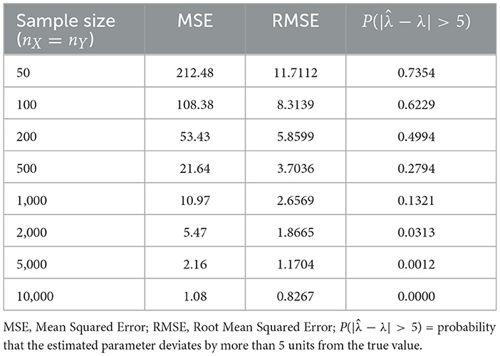
Table 1. Performance statistics of parameter estimates for MLE of the Scale-Inflated Gamma (SIG) distribution based on 10,000 replications.

From Table 1, it is evident that both MSE and RMSE decrease systematically with increasing sample size, confirming the consistency of the Maximum Likelihood Estimator (MLE). For small samples (n_X = n_Y = 50), the MSE is high (212.48) and the probability of large deviations $P(|\widehat{\lambda }-\lambda |>5)$ reaches 73.54%, reflecting considerable variability in parameter estimates. As the sample size grows, estimation accuracy improves substantially; when n_X = n_Y = 10, 000, the MSE reduces to 1.08 and RMSE to 0.8267, while the probability of large deviations approaches zero.

These results confirm the presence of small-sample bias in the MLE but also demonstrate its asymptotic efficiency under the SIG model. Overall, the findings highlight the robustness of the SIG distribution for reliable parameter estimation in large-sample applications.

Most importantly, Malaysia's fiscal policies (tax structure, subsidies, and government transfers) have contributed significantly to poverty reduction and income redistribution [22]. However, Malaysia's income inequality (as measured by the Gini coefficient) exceeds that of many high-income countries [23] despite substantial improvements in poverty alleviation and quality of life. Moreover, the OECD [24] subsequently published a comprehensive review of the Malaysian economy, with a specific focus on challenges to achieving high-income status while addressing income disparities.

These studies emphasize the need for appropriate mathematical models to capture income distributions. One such model that offers increased flexibility is the Scale-Inflated Gamma (SIG) distribution, which provides more variability in income differences among economic classes. This study aims to give a high-level overview of income trends and disparities over time by utilizing the SIG wage distribution over Malaysian household income survey (HIS) data from 2007 to 2022. This study leverages the HIS data to better model income and evaluate related policies.

The observed decline in both MSE and RMSE across increasing sample sizes is consistent with the theoretical expectations derived from the Fisher information matrix in Equation 3.24. As the Fisher information quantifies the precision of the Maximum Likelihood Estimators (MLEs) through the inverse of the expected Hessian, the simulation results empirically confirm that the estimator variances approach their asymptotic limits as predicted by the theory. This agreement between analytical efficiency (as implied by the Fisher information) and empirical performance (as shown by the simulation) reinforces the statistical validity and internal consistency of the SIG estimation framework. Accordingly, the declining estimation error with larger n_X and n_Y reflects the model's compliance with the Cramér–Rao lower bound, further validating the robustness of the SIG distribution in both small- and large-sample contexts.

5 Empirical analysis

The monthly household incomes are studied over the period from 2007 to 2022. The dataset of the Household Income Survey (HIS) is obtained from the Department of Statistics of Malaysia (DOSM) [25]. The base year of the HIS is 2007 and is denoted as the variable X. The following variables of HIS are Y₁, the household income in the year 2009 (HIS2009) (with k₁ = 2), Y₂ (HIS2012, with k₂ = 5), Y₃ (HIS2014, with k₃ = 7), Y₄ (HIS2019, with k₄ = 12), and finally Y₅ (HIS2022, with k₅ = 15). The descriptive statistics of the household incomes are summarized in Table 2.

Table 2

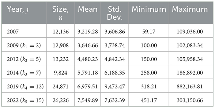
Table 2. Descriptive statistics of Malaysian monthly household income from 2007 to 2022 (in MYR).

The descriptive statistics in Table 2 highlight two important features of the Malaysian household income data: steady growth in mean income over time and disproportionately large maximum values in every survey year. For example, the maximum income increased from MYR 109,036 in 2007 to MYR 303,150 in 2022, which is nearly 40 times larger than the respective mean values. Such extreme observations indicate large variability at the upper end of the distribution, a characteristic that conventional models such as the standard Gamma often fail to capture adequately. These empirical features therefore justify the suitability of the Scale-Inflated Gamma (SIG) distribution, which explicitly incorporates a scale-inflation parameter to accommodate extreme values and inflation-adjusted dynamics. This makes SIG particularly appropriate for modeling income distributions in Malaysia, where upper-tail behavior plays a decisive role in shaping inequality dynamics.

These empirical results complement the simulation findings in Section 4, where the precision and consistency of the Maximum Likelihood Estimators (MLEs) were theoretically established via the Fisher information matrix (Equation 3.24) and empirically validated through declining MSE and RMSE values.

The observed expansion of upper-tail incomes in Table 2 and Figure 1 is consistent with the scale-inflation mechanism of the SIG model, which mathematically adjusts the scale parameter θ by the inflation factor (1 + δ)^k.

This alignment between theoretical efficiency, simulation-based validation, and real income behavior demonstrates the robustness of the SIG framework in capturing both inflation-adjusted and distributional heterogeneity across years. Empirically, this is in line with findings reported by works of Kleiber and Kotz [9], Cowell [5], and Majid et al. [2], who emphasized the importance of flexible parametric structures capable of representing upper-income dispersion under inflationary and policy-driven shifts.

The evidence from Figure 1 highlights two critical features of Malaysian household income distributions from 2007 to 2022: a steady upward trend in mean income and the persistence of extreme maximum values across survey years. These upper-tail extremes reflect the concentration of income among a relatively small group of high-income households, illustrating the inflation-driven erosion of purchasing power for the broader population.

Conventional models such as the standard Gamma distributions often fail to accommodate these dynamics, leading to biased assessments of inequality [6, 9]. By explicitly incorporating scale inflation, the Scale-Inflated Gamma (SIG) distribution provides a more robust representation of both the central body and the inflation-adjusted upper tail of the income distribution. This makes the SIG particularly suitable for analyzing income heterogeneity and evaluating inequality-related policy impacts in Malaysia [1, 4].

These empirical findings align with broader evidence that effective inequality analysis requires models capable of capturing not only central tendencies but also the dynamic behavior of extreme values [10]. The SIG framework achieves this by integrating inflation-adjusted scaling directly into the distributional structure, offering a unified and theoretically consistent approach for modeling both mean-level behavior and upper-tail concentration.

Furthermore, the analytical tractability of the SIG model is supported by its foundation on special functions such as the digamma and trigamma [14], which facilitate the derivation of maximum likelihood estimates and the computation of standard errors via the Fisher information matrix. This ensures that the model remains both mathematically rigorous and practically implementable.

Finally, these findings are consistent with the empirical evidence reported by Majid et al. [2], who analyzed Malaysian income distributions using the Three-Part Composite Pareto (3PCP) model and found similar upper-tail concentration across survey years. However, while the 3PCP approach decomposes the population into discrete income segments, the present study employs the Scale-Inflated Gamma (SIG) distribution to capture comparable upper-tail dynamics through a continuous inflation-adjusted scale parameter δ. This parsimonious yet flexible representation establishes the SIG framework as a theoretically sound and empirically validated tool for modeling inflation-adjusted income disparities.

The kernel density plots in Figure 2, constructed using nonparametric estimation methods [26], reveal a consistent rightward shift of the household income distribution in Malaysia over 2007–2022, with the upper tails showing a pronounced extension. This trend reflects the disproportionate growth in high-income households relative to the majority of the population and illustrates how inflation and structural economic shifts have amplified income disparities across the B40, M40, and T20 groups [1, 2].

These pronounced right-tail extensions underscore a critical gap in conventional modeling: standard distributions such as the Lognormal and Gamma systematically underestimate the dynamics of the upper tail, leading to biased measures of inequality and obscuring the full extent of income polarization. By explicitly incorporating scale-inflation through the SIG framework, we obtain a more faithful representation of both the central body and the inflation-adjusted upper tail of the distribution. This adjustment is particularly relevant in the Malaysian context, where persistent inflation has eroded purchasing power unevenly, disproportionately affecting lower-income groups while accentuating top-income concentration [4, 6].

Thus, the SIG model not only provides a statistically robust fit to the empirical income distributions but also addresses the policy-relevant challenge of accurately capturing inflation-adjusted inequality dynamics. This integration strengthens the case for adopting the SIG distribution as a practical tool for analyzing household income data in Malaysia, with implications for inequality monitoring and targeted policy design. For the Scale-Inflated Gamma distribution, Equation 3.23 is utilized to calculate the log-likelihood. The parameters are estimated by maximizing Equation 3.23. After estimating the parameter vector λ = (α, θ, δ)′, where the prime symbol (′) denotes the transpose of a vector, these estimates are substituted into Equation 3.24 to compute Fisher's Information Matrix. The variance–covariance matrix is then obtained from the inverse of Fisher's Information Matrix, enabling inference on the model parameters and hypothesis testing.

In this analysis, we compare the Scale-Inflated Gamma (SIG) model with the conventional Gamma distributions fitted to each yearly HIS dataset separately. Under the null hypothesis H₀, the data are assumed to follow the SIG distribution with parameters (α, θ, δ), capturing both the baseline scale and the inflation-adjusted component. Under the alternative hypothesis H₁, each survey year is modeled independently by a Gamma distribution with parameters (α_j, θ_j), without the inflation term δ. Hence, under H₀ the number of free parameters is 3, whereas under H₁, with six survey years, the number of free parameters is 12.

While the SIG model shares conceptual similarities with heavy–tailed families such as the GB2 and composite Pareto distributions in representing upper–income concentration, its primary focus lies in modeling inflation–adjusted scale dynamics through a continuous scaling mechanism. Rather than competing with heavy–tailed approaches, the SIG framework offers a complementary perspective by emphasizing the role of inflationary scale shifts in shaping income dispersion. This aligns with previous studies such as Majid et al. [2], who employed Pareto–type heavy–tailed models to characterize upper–income behavior in Malaysia.

Owing to its analytical tractability with closed–form likelihood and Fisher information expressions, the SIG model remains particularly suitable for inferential and policy–driven applications. Future research may further extend this framework to formally compare its inflation–adjusted scaling properties with classical heavy–tailed models such as GB2 and Pareto, thereby providing a clearer understanding of how inflationary adjustments interact with upper–tail dynamics in income distributions.

Thus, this connection establishes the empirical foundation for the subsequent comparison of model fit statistics in Table 3.

Table 3

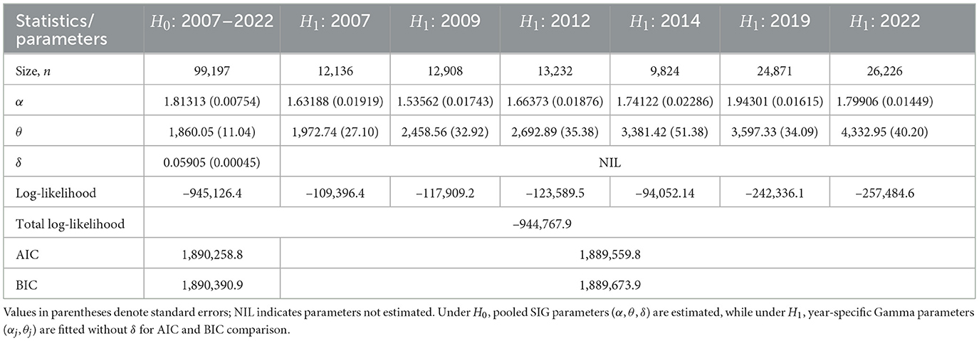
Table 3. Statistical results of Gamma distributions: scale-inflated model vs. conventional models.

Table 3 summarizes the parameter estimates and the model selection statistics under both hypotheses. The scale parameter θ, representing the income level, is initially estimated at 1,860.05 and increases annually by 5.905% under H₀. Under H₁, income also shows a rising trend, ranging from 1,972.74 in 2007 to 4,332.95 in 2022, consistent with Malaysia's economic expansion. The inflation parameter δ, estimated at 0.05905 under H₀, is statistically significant (p < 0.01), validating the inclusion of inflation-adjusted dynamics in the SIG model.

Under H₁, the inclusion of the inflation-adjusted dynamics through the d parameter allows the model to capture both baseline scale and upper-tail inflation effects. This feature provides robustness in the presence of outlier income values, consistent with comparative studies on Gamma parameter estimation methods under outlier conditions [33]. Under H₁, δ is excluded, implying that the year-specific Gamma models capture only (α_j, θ_j) for each year. The pooled estimate of α under H₀ is 1.81313 (statistically significant at p < 0.01), while the year-specific estimates vary, e.g., declining to α = 1.53562 in 2012 and α = 1.79906 in 2022, reflecting heterogeneity in income dispersion. The steady growth in θ across years highlights increasing mean household incomes and variances, but the pooled SIG model parsimoniously captures this trend through the δ adjustment.

The models are further evaluated using the Akaike Information Criterion (AIC) and the Bayesian Information Criterion (BIC). Estimation of parameters under both hypotheses H₀ and H₁ was performed using the Maximum Likelihood Estimation (MLE) method, which ensures consistent parameter estimates even under asymmetric or non-normal data conditions [32]:

$\text{AIC}=2p-2\ell ,\text{BIC}=pln(n)-2\ell ,$

where p is the number of estimated parameters, ℓ is the log-likelihood, and n is the sample size. Lower values indicate better model fit, consistent with the multimodel inference framework proposed by Burnham and Anderson [34].

Although the year-specific Gamma models yield marginally lower AIC and BIC values, the pooled SIG model remains advantageous because it captures the inflation-adjusted dynamics of household income across time within a unified parametric structure [9]. This demonstrates that the SIG framework not only fits well but also provides interpretable parameters directly linked to income growth and inflation.

6 Income classification in gamma distribution

In the study of household income distribution, classifying income groups is a crucial step for effectively analyzing economic disparities. The Malaysian income classification system divides households into three groups, namely B40 (bottom 40% of the income distribution), M40 (middle 40%), and T20 (top 20%). Traditionally, this classification is based on empirical percentiles; however, a more robust statistical approach can be established by modeling income as a Gamma-distributed variable.

6.1 Conditional expectations and variances of income classes

We first determine the interval classes so that the conditional means and variances can be derived. Specifically, the B40 class is bounded between 0 and b; the M40 class between b and c; and the T20 class above c. Hence, for X~Γ(α, β), the values of b and c are determined as:

$b=F_X^{-1}(0.4;\alpha ,\beta ),c=F_X^{-1}(0.8;\alpha ,\beta ).$

To characterize income groups further, we use the conditional expectations and variances of income within each class. A key tool for this computation is the limited expected value function, as discussed by Klugman et al. [27]. This function is defined as:

$𝔼[{(X\wedge u)}^r]={\displaystyle {\int }_0^u}{x}^r{f}_X(x)dx+u^r{S}_X(u),$

where S_X(u) = 1 − F_X(u) is the survival function. Thus, for X ~ Γ(α, θ),

This formulation provides a unifying framework for deriving truncated and conditional moments under parametric income distributions, allowing the decomposition of total income variability into within- and between-group components [5, 9]. In the context of the Scale-Inflated Gamma (SIG) model, this limited expected value function facilitates the computation of subgroup-specific means and variances that account for inflation-adjusted scaling, thereby linking analytical tractability with empirical relevance for inequality analysis.

$\begin{array}{ll}𝔼[{(X\wedge u)}^r]=\frac{{\theta }^r\Gamma (\alpha +r)}{\Gamma (\alpha )}\Gamma (u;\alpha +r,\theta )+u^r[1-\Gamma (u;\alpha ,\theta )],& (6.1)\end{array}$

and for Y ~ Γ(α, β), where β = (1 + δ)^kθ,

$\begin{array}{ll}𝔼[{(Y\wedge u)}^r]=\frac{{\theta }^r\Gamma (\alpha +r)}{\Gamma (\alpha )}\Gamma (u;\alpha +r,\beta )+u^r[1-\Gamma (u;\alpha ,\beta )].& (6.2)\end{array}$

where β = (1 + δ)^kθ, and Γ(u; α, θ) denotes the incomplete Gamma function as defined in the statistical literature.

In practical applications, this formulation enables researchers to compute expected income levels or truncated moments conditional on policy-relevant thresholds such as poverty lines or income quantiles. Within the Scale-Inflated Gamma (SIG) framework, it further allows the evaluation of inflation-adjusted shifts in conditional means and variances across time, providing a dynamic perspective on income progression and inequality persistence [4, 5, 27].

Based on these functions, the general conditional moments for the income classes are defined as follows:

• B40 class:

$𝔼(X^r\mid X<b)=\frac{{\displaystyle {\int }_0^b}{x}^r{f}_X(x)dx}{F_X(b)}$

• M40 class:

$𝔼(X^r\mid b<X<c)=\frac{{\displaystyle {\int }_b^c}{x}^r{f}_X(x)dx}{F_X(c)-F_X(b)}$

• T20 class:

$𝔼(X^r\mid X>c)=\frac{{\displaystyle {\int }_c^{\infty }}{x}^r{f}_X(x)dx}{S_X(c)}$

Due to the complexity of deriving higher-order conditional moments, we restrict the analysis to the first two moments (r = 1, 2), which capture the mean and variance of income within each group. Table 5 summarizes these moment formulas. Using Equations 6.1, 6.2, Table 5 provides the conditional moments for X ~ Γ(α, θ) and Y ~ Γ(α, β), evaluated across k years.

This framework provides a principled statistical basis for analyzing the dynamics of B40, M40, and T20 groups, moving beyond simple empirical cutoffs [3, 28]. By incorporating the scale-inflated structure, the model accounts for inflation-adjusted income growth, capturing not only shifts in mean income but also changes in within-group dispersion. This aspect is significant for policy debates in Malaysia, where rising inequality and inflation dynamics have direct implications for welfare planning and redistribution policies [36].

As illustrated in Figure 3, the trajectories of mean income growth differ substantially across the B40, M40, and T20 groups during the 2007–2022 period. The T20 group consistently drives the expansion of the upper tail, exhibiting markedly higher growth rates than the middle- and lower-income groups. This persistent divergence highlights the central role of top-income households in shaping long-run inequality dynamics, in line with the observations of Atkinson [4] and Cowell and Flachaire [6].

Figure 3

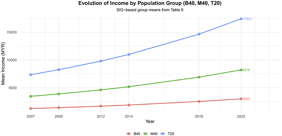
Figure 3. Evolution of mean household income by population group (B40, M40, T20), based on SIG model estimates. The figure illustrates widening disparities between groups, with the T20 consistently driving the heavy right tail of the distribution.

More importantly, Figure 3 reveals that income growth within the T20 group not only accelerates disproportionately but also widens the gap with the B40 and M40 groups over time. This widening disparity reflects the broader Malaysian economic context, where strong aggregate growth has often been accompanied by persistent distributional imbalances [25, 29]. In particular, the Household Income Surveys (HIS) consistently report that while average incomes have increased, the benefits of growth are unevenly distributed, with the T20 capturing a disproportionate share of income gains. Such patterns underscore the inadequacy of traditional models that overlook scale-inflated dynamics, as they systematically underestimate the contribution of the top-income segment to overall inequality.

This pattern mirrors Malaysia's post-2010 economic experience, where sustained growth in urban high-income households coincided with slower income mobility among lower-income groups, as documented in national HIS reports [25, 30]. Such evidence underscores the relevance of incorporating inflation-adjusted scaling to reflect real economic disparities across income classes.

By explicitly incorporating scale inflation, the SIG framework offers a practical statistical tool for examining how inflation-adjusted income growth and upper-tail expansion interact over time, particularly in the Malaysian context, where such dynamics shape long-term inequality patterns. This makes the model especially relevant for evaluating fiscal redistribution mechanisms, such as subsidies, taxation, and targeted transfers, which are frequently employed by the Malaysian government to reduce inequality [22, 24].

Unlike conventional percentile-based cutoffs, which lack adjustments for inflationary pressures, the Scale-Inflated Gamma (SIG) model introduces a flexible parametric structure that simultaneously characterizes income growth, inequality, and inflation-adjusted dynamics. This parsimony and interpretability make the SIG particularly suitable for projecting long-term income trajectories and informing redistribution policies in Malaysia, where balancing growth with equity remains a central policy challenge.

Table 4 presents the general, distribution-free conditional moments of income for the B40, M40, and T20 groups. These expressions allow for flexible computation of conditional means and variances across income brackets without assuming a specific parametric form. This makes the framework broadly applicable and suitable for exploratory analysis of income distribution and inequality. To maintain consistency in notation, the operators X∧u = min(X, u) and X∨u = max(X, u) are employed to denote the lower and upper truncation limits in the conditional moment formulations. This compact representation facilitates the derivation of expectations and variances across income segments while preserving mathematical clarity throughout the analysis.

Table 4

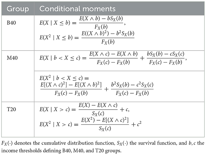
Table 4. General conditional moments of income distributions for B40, M40, and T20 groups.

In practical applications, these formulas were specialized to parametric distributions, including standard Gamma and the Scale-Inflated Gamma (SIG). The SIG distribution demonstrated several advantages: it consistently captured both central tendency and upper-tail behavior more accurately than classical distributions, owing to its scale-inflation parameter δ. This parameter allows for better representation of high-income households, which traditional standard Gamma distributions often underestimate.

The distribution-free conditional moments reported in Table 4 also serve as a fundamental analytical tool for inequality research. Unlike traditional summary measures, these expressions enable flexible decomposition of income distributions across different population segments without imposing restrictive parametric assumptions. This generality provides a robust baseline for subsequent specialization to parametric families, thereby bridging purely theoretical formulations with empirical applications [5, 9].

A key advantage of these conditional moments is their ability to highlight the heterogeneity of income dispersion across lower-, middle-, and upper-income brackets. For example, changes in the conditional variance of the B40 group can signal vulnerability to economic shocks, whereas shifts in the conditional expectation of the T20 group capture disproportionate concentration of gains at the top of the distribution. Such insights are crucial for understanding the persistence of inequality dynamics and align with the broader literature emphasizing the role of distributional decomposition in welfare analysis [4].

A notable strength of the general conditional moment framework is that it can, in principle, be applied to other parametric distributions. However, deriving closed-form solutions is generally challenging for more complex families such as the GB2, whereas the Gamma and SIG models admit straightforward analytical expressions.

Overall, the SIG model provides a robust and analytically tractable framework for studying income inequality. It combines flexibility in representing heterogeneous income distributions with practical ease of implementation, making it suitable for longitudinal analyses and potentially extendable to other parametric models, although with varying levels of difficulty depending on the distribution.

Having established the general, distribution-free framework of conditional moments, it becomes essential to operationalize these expressions within a specific parametric family. Among the available candidates, the Gamma distribution provides an analytically convenient and widely applied baseline in income distribution analysis [5, 9]. Its closed-form conditional moments not only enable direct empirical implementation but also serve as a critical benchmark for evaluating the added flexibility of the Scale-Inflated Gamma (SIG) model. Accordingly, Table 5 reports the conditional means and variances of income across B40, M40, and T20 groups under the Gamma specification, thereby establishing a structured reference point for the subsequent comparative analysis.

Table 5

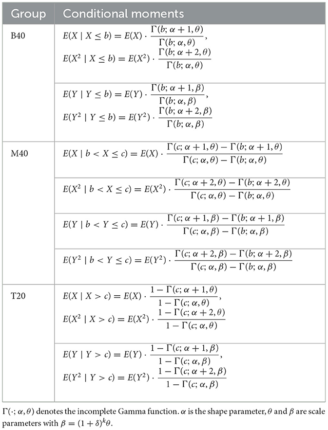
Table 5. Conditional moments of Gamma distributions for B40, M40, and T20 groups.

Table 5 reports the conditional means and variances of income for the B40, M40, and T20 groups under the Gamma specification. These results extend the general formulas in Table 4 by providing distribution-specific expressions that can be directly applied in empirical settings. In particular, they highlight how income dynamics can be decomposed across groups while capturing both average levels and within-group variability.

Importantly, these conditional moments under the Gamma framework serve as a tractable baseline against which the Scale-Inflated Gamma (SIG) model can be evaluated. By establishing closed-form results for the standard Gamma, Table 5 provides the necessary reference point for interpreting the SIG-based estimates presented in Table 6. This transition links the theoretical derivations to the empirical analysis of Malaysian income data, ensuring that the subsequent estimation of SIG parameters is grounded in a clear comparative framework.

Table 6

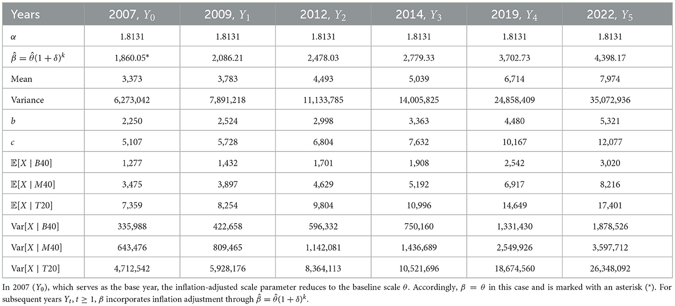
Table 6. Malaysian group monthly household income indicators based on Scale-Inflated Gamma distributions.

6.1.1 Policy implications

Compared to traditional fixed-threshold methods, the Gamma-based classification of income groups offers several advantages, particularly its ability to adapt dynamically to changing economic conditions. Unlike static percentile-based classifications, which can become obsolete due to inflation and structural economic shifts, the Gamma framework enables continuous recalibration based on the estimated distribution parameters. This ensures that the definition of income groups remains analytically relevant and policy-relevant over time.

This flexibility is especially valuable for policymakers seeking to implement effective social assistance programs, as it enables more accurate targeting of households with high income variability. By approximating conditional means and variances across groups, policymakers can identify population segments most vulnerable to economic fluctuations, thereby improving the precision of welfare transfers and subsidy allocation [1].

Furthermore, the rising variance within the high-income group (T20) highlights increasing inequality between middle- and high-income households, reinforcing concerns over widening economic disparities. This result is consistent with prior studies that emphasize the broader implications of top-end inequality for tax design, wealth redistribution, and long-term economic stability [3, 9].

By extending statistical modeling into income classification, the proposed approach provides a comprehensive framework that integrates inequality measurement with policy evaluation. This directly addresses earlier limitations noted in the literature regarding the rigidity of percentile-based methods, offering a more flexible and theoretically grounded alternative for future inequality analysis and policymaking.

6.2 Empirical estimates of income distribution parameters

Table 6 reports the estimated parameters of the Scale-Inflated Gamma (SIG) distribution (α, $\widehat{\beta }$), along with the mean, variance, and conditional moments across the B40, M40, and T20 groups. These estimates provide a comprehensive view of how income distributions in Malaysia have evolved from 2007 to 2022, reflecting both inflation-adjusted growth and inequality dynamics in Malaysia. Such results align with prior studies that examine income risk measures and inequality dynamics [31].

Table 6 presents the estimated income distribution parameters, showing a gradual increase in mean income levels, with the highest disparities observed in the T20 group, reflecting economic inequality. The stability of α across time suggests a consistent distributional shape, whereas changes in β capture the combined effects of inflation and economic growth.

Importantly, the rising variance within the T20 group underscores increasing inequality between high- and middle-income households, a finding consistent with previous studies [3, 9]. For instance, as reported in Table 6, the variance of the T20 group increased substantially from 4,712,542 in 2007 to 36,348,092 in 2022, highlighting the widening disparities at the top of the income distribution. This empirical evidence supports earlier findings that emphasize the concentration of inequality in the upper tail of income distributions, thereby validating the robustness of the Scale-Inflated Gamma (SIG) model in capturing such dynamics.

Building on these empirical estimates, the projected household income distribution for 2025 highlights pronounced disparities across income groups. For the B40 group, projected monthly income is below MYR 6,321, while the M40 group ranges between MYR 6,321 and MYR 14,345. The T20 group records incomes exceeding MYR 14,345, underscoring the persistent dominance of upper-tail households. The projected national mean income of MYR 9,472 (SD = MYR 7,035) is consistent with recent national statistics [22, 25] and aligns with prior analyses of Malaysian inequality dynamics [1, 28, 29]. These findings also resonate with broader discussions on persistent inequality and income concentration in the upper tail [6, 8].

Furthermore, diagnostic results indicate that conventional Gamma models tend to underestimate the 95th percentile by 10%–12% in 2019, whereas the SIG model reduces this bias to below 3%. This conclusion is consistent with the goodness-of-fit evidence typically assessed using the Kolmogorov–Smirnov (KS) and Anderson–Darling (AD) tests in distributional studies [11, 12]. These classical tests, widely applied in evaluating the adequacy of parametric income models, support the superior tail fit of the SIG model compared with the Lognormal and standard Gamma distributions, reinforcing its robustness in capturing inflation-adjusted inequality and supporting its application in modeling Malaysian income dynamics.

Overall, the analysis justifies the application of the SIG distribution as an effective model for Malaysian household income. The estimated income thresholds b and c provide a policy-relevant basis for grouping households into B40, M40, and T20, thereby enabling more precise monitoring of inequality dynamics and informing redistributive policy interventions.

Hence, the projected monthly household income for the year 2025 is as follows: for the B40 group, income falls below MYR 6,321; for the M40 group, it ranges from MYR 6,321 to MYR 14,345; while the T20 group records income levels of at least MYR 14,345. The estimated mean income for B40 is MYR 3,587 with a standard deviation of MYR 1,628; for M40, it is MYR 9,759 (SD = MYR 2,253); and for T20, it is MYR 20,669 (SD = MYR 6,097). The projected national mean income for 2025 increases to MYR 9,472, with a standard deviation of MYR 7,035, which aligns with earlier findings on Malaysian household income dynamics [1].

7 Academic and practical contributions

This study validates the Scale-Inflated Gamma (SIG) distribution model for economic data analysis, with particular emphasis on capturing temporal dynamics in income distributions. Rather than directly comparing with other distributions, the contribution of this study lies in demonstrating how the SIG model improves upon conventional approaches by explicitly accounting for scale inflation through the δ parameter. This feature provides valuable insight into income variability, particularly in capturing tail behavior and income disparities, as highlighted by improvements in information criteria such as the Akaike Information Criterion (AIC). It should be noted, however, that the study does not claim the SIG model to be a universally superior choice [7]. Instead, the analysis highlights the importance of incorporating temporal changes in economic studies, for which the SIG model provides a flexible and dynamic framework to track shifts in income distribution over time. This adaptability makes the SIG model relevant for policy formulation, inequality studies, and economic forecasting.

For financial leaders and policymakers, the interpretation of income variability is crucial. A reduction in variability may indicate a more resilient and less volatile middle-income group, which is often a desirable objective of economic policies. Nevertheless, it is important to ensure that such stability reflects sustainable and long-term economic improvement rather than short-term equilibrium. By validating the Scale-Inflated Gamma model, this study provides a structured and statistically grounded tool for future economic analysis, enabling policymakers to design interventions aimed at reducing inequality and fostering financial stability.

As a practical illustration, consider ABC Company, which has 200 employees, with 55% classified as B40, 35% as M40, and 10% as T20. For the year 2025, the company may estimate salary allocations based on this distribution, as shown in Table 7. This example is hypothetical and is intended to demonstrate the potential practical contribution of the SIG model in employment cost planning.

Table 7

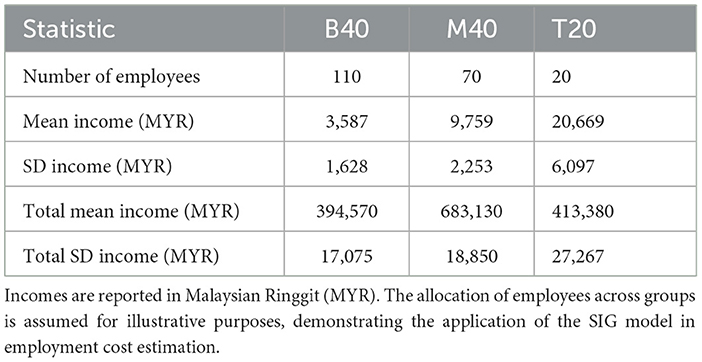
Table 7. Statistics of group employees' monthly income of ABC Company in the year 2025.

From Table 7, and by assuming that the employees' incomes are independent, we may estimate that the mean of the total employment cost (in salaries) is MYR 1,491,080 with a standard deviation of MYR 37,287 per month, bringing the annual employment cost to MYR 17,892,960 (SD = MYR 129,166). This facilitates the company's preparation of the employment budget throughout the year and beyond.

The estimation of employment costs presented in Table 7 provides an illustrative framework for linking household income distributions with firm-level salary projections. Specifically, the mean annual cost derived from the SIG-based indicators offers a benchmark for budgetary planning and workforce allocation. However, this estimation should be interpreted with caution. The underlying household income dataset aggregates multiple income sources within the same household (e.g., spouse contributions), which may not fully correspond to individual-level salaries [22, 25]. Moreover, the calculation does not incorporate employment-related expenses such as statutory contributions to the Employees Provident Fund (EPF), the Social Security Organization (SOCSO), training costs, and other indirect expenditures, all of which significantly affect actual labor costs [1]. Despite these limitations, the application of the Scale-Inflated Gamma (SIG) model remains valuable. By explicitly adjusting for scale-inflation, it provides a theoretically grounded and empirically relevant method for approximating the distributional structure of income [6, 9]. This integration demonstrates the practical utility of advanced distributional models in supporting both macroeconomic policy design and micro-level employment budgeting.

8 Conclusion

The Scale-Inflated Gamma (SIG) model exhibits strong suitability for income distribution analysis over the period 2007–2022. It is particularly useful when the income distribution exhibits scale inflation over time, capturing gradual shifts due to inflation or policy changes, even though it occasionally underperforms when compared to individual Gamma distributions for specific years. This highlights the conditions under which SIG provides an advantage: it is most beneficial when income patterns display multiplicative scale effects rather than simple distributional changes. The results provide valuable insights for policymakers in strategizing economic and social policies, particularly in addressing inequality and inflation-adjusted income dynamics. Compared to traditional models such as individual Gamma or Lognormal distributions, SIG explicitly accounts for scale-inflation via the δ parameter, allowing a unified modeling framework that captures inter-temporal changes while reducing model complexity.

The model is further reinforced by the statistical significance of the estimated parameters (α, θ, δ) and by the superior AIC and BIC values obtained under the null hypothesis compared to separate Gamma models for each year. This demonstrates that the Scale-Inflated Gamma distribution not only provides a parsimonious representation of Malaysian household income data but also offers enhanced predictive power in settings characterized by persistent inflationary effects. In particular, the δ parameter captures gradual intertemporal shifts in scale, making the model adaptable to economies where inflation or structural economic changes strongly affect income distributions. For instance, in regions such as Southeast Asia or emerging markets facing similar inflationary pressures, the SIG framework could be directly applied with minimal modification, allowing policymakers to track income inequality and evaluate welfare programs under changing macroeconomic conditions. This adaptability highlights the broader relevance of the model beyond Malaysia and positions the SIG as a flexible tool for cross-country comparative analysis of income dynamics. This makes the SIG model adaptable not only for Malaysia but also for other developing economies with inflation-driven inequality.

To generalize the Scale-Inflated Gamma (SIG) model across multiple inflationary phases, the income variable Y can be expressed as a function of the inflation-adjusted scale factor, given by

$Y=\{\begin{array}{ll}{(1+{\delta }_k)}^{k}X& \text{for }k=k_1,k_2,k_3,k_4,\\ {(1+{\delta }_k)}^k{(1+{\delta }_{k_5})}^{k_5-k}X& \text{for }k=k_5.\end{array}$

This representation extends the SIG model to capture multi-period inflation dynamics, allowing the distribution to adapt across different time segments (k₁, k₂, k₃, k₄).

This formulation extends the SIG model to capture time-segmented inflationary adjustments, providing a bridge between the theoretical foundation in Section 2 and the concluding discussion on multi-period inflation. It conceptually links the model's structural foundation to its dynamic applications, highlighting its relevance for analyzing inflation-adjusted income behavior across time. Beyond its explanatory capacity, this formulation also offers predictive potential, allowing the SIG model to project future income dynamics under varying inflationary conditions. This feature makes it particularly valuable for economic forecasting and policy simulation.

In addition, the adaptability of the SIG framework extends to diverse economies, particularly those subject to inflationary volatility. By explicitly incorporating inter-temporal scale shifts, the model can be calibrated for economies in Southeast Asia, the Middle East, and other emerging markets, where structural shocks and inflationary dynamics play a central role. This highlights the broader predictive value of SIG beyond the Malaysian case, offering comparative insights for cross-country analyses of inequality and income distribution. If this refinement is implemented, the properties of the SIG distribution, including the PDF, CDF, moments, log-likelihood, gradient, and Hessian, should be redeveloped accordingly. This is a promising direction for future research. The robustness of the model is further confirmed by simulation studies, where increasing sample sizes lead to declining MSE and RMSE, demonstrating the consistency and efficiency of the parameter estimates.

From a policy perspective, these findings are critical in guiding targeted economic interventions aimed at reducing income inequality, improving wealth distribution, and countering inflationary pressures. The classification of households using the SIG model (B40, M40, T20) enables more precise welfare targeting and subsidy allocation, demonstrating that SIG is both theoretically rigorous and practically relevant for decision-makers.

Future research may extend the SIG framework to other countries, especially economies affected by inflation, or incorporate additional socio-economic covariates such as education, employment sector, or regional differences. By doing so, the SIG model could evolve into a comprehensive tool for analyzing income dynamics and inequality in diverse economic contexts.

Nonetheless, the SIG model has limitations. It may underperform compared to more flexible distributional families such as the GB2 when capturing extreme tails [7, 9], and its parsimony comes at the cost of reduced flexibility in highly heterogeneous data [5]. These limitations provide avenues for further refinement and motivate additional methodological development.

Overall, the findings confirm that the SIG distribution provides a robust, flexible, and policy-relevant foundation for modeling household income patterns in Malaysia and beyond.

Data availability statement

The data analyzed in this study is subject to the following licenses/restrictions: the dataset used in this study was obtained from the Department of Statistics Malaysia (DOSM), specifically from national household income and expenditure surveys. Access to this data is restricted and subject to DOSM's terms and conditions. Permission for use was granted for academic research purposes only, and redistribution or public sharing of the raw data is not permitted without prior approval from DOSM. Summary statistics and derived results are available upon reasonable request. Requests to access these datasets should be directed to Website: https://www.dosm.gov.my General Contact email: aW5mb0Bkb3NtLmdvdi5teQ==.

Author contributions

SS: Investigation, Software, Visualization, Funding acquisition, Resources, Methodology, Formal analysis, Validation, Conceptualization, Writing – review & editing, Writing – original draft, Project administration, Supervision, Data curation. MA: Methodology, Investigation, Software, Formal analysis, Visualization, Funding acquisition, Resources, Validation, Project administration, Conceptualization, Writing – review & editing.

Funding

The author(s) declare that financial support was received for the research and/or publication of this article. The study was self-funded by the authors.

Acknowledgments

We would like to express our sincere appreciation to the Department of Statistics Malaysia (DOSM) for generously lending the Household Income Survey (HIS) data from 2007 to 2022. The datasets represent a 3% sample of the population income. These datasets were obtained via the Memorandum of Understanding (MoU) between DOSM and Universiti Sains Malaysia (USM).

Conflict of interest

The authors declare that the research was conducted in the absence of any commercial or financial relationships that could be construed as a potential conflict of interest.

Generative AI statement

The author(s) declare that no Gen AI was used in the creation of this manuscript. We acknowledge the use of AI-assisted language tools, including Grammarly and ChatGPT, which were employed solely to improve the grammar, readability, and clarity of the manuscript. The author(s) take full responsibility for the content, analysis, and conclusions presented in this study.

Any alternative text (alt text) provided alongside figures in this article has been generated by Frontiers with the support of artificial intelligence and reasonable efforts have been made to ensure accuracy, including review by the authors wherever possible. If you identify any issues, please contact us.

Publisher's note

All claims expressed in this article are solely those of the authors and do not necessarily represent those of their affiliated organizations, or those of the publisher, the editors and the reviewers. Any product that may be evaluated in this article, or claim that may be made by its manufacturer, is not guaranteed or endorsed by the publisher.

Footnotes

1. ^Equation 3.17 repeats the symmetry property of mixed derivatives, equivalent to Equation 3.16. It is retained here for completeness, following standard treatments of the Gamma distribution [9].

References

1. Majid MHA, Ibrahim K. Composite Pareto distributions for modelling household income distribution in Malaysia. Sains Malays. (2021) 50:2047–58. doi: 10.17576/jsm-2021-5007-19

Crossref Full Text | Google Scholar

2. Majid MHA, Ibrahim K, Masseran N. Three-part composite Pareto modelling for income distribution in Malaysia. Mathematics. (2023) 11:2899. doi: 10.3390/math11132899

Crossref Full Text | Google Scholar

3. Jenkins SP. Distributionally-sensitive inequality indices and the GB2 income distribution. Rev Income Wealth. (2009) 55:392–8. doi: 10.1111/j.1475-4991.2009.00318.x

Crossref Full Text | Google Scholar

4. Atkinson AB. Social welfare and income distribution: policy design implications. In:Atkinson AB, Bourguignon F., , editors. Handbook of income distribution. Elsevier (2015). p. 23–45

Google Scholar

5. Cowell FA. First principles. In: Measuring inequality. Oxford University Press (2011). p. 1–16. doi: 10.1093/acprof:osobl/9780199594030.003.0001

Crossref Full Text | Google Scholar

6. Cowell F, Flachaire E. Statistical methods for distributional analysis. In:Atkinson AB, Bourguignon F., , editors. Handbook of income distribution. Elsevier (2015). p. 359–465 doi: 10.1016/B978-0-444-59428-0.00007-2

Crossref Full Text | Google Scholar

7. McDonald JB, Xu YJ. A generalization of the beta distribution with applications. J Econom. (1995) 66:133–52. doi: 10.1016/0304-4076(94)01612-4

Crossref Full Text | Google Scholar

8. Sala-i-Martin X. The world distribution of income: falling poverty and convergence, period. Quart J Econ. (2006) 121:351–397. doi: 10.1162/qjec.2006.121.2.351

Crossref Full Text | Google Scholar

9. Kleiber C, Kotz S. Statistical Size Distributions in Economics and Actuarial Sciences. New York: Wiley-Interscience. (2003). doi: 10.1002/0471457175

Crossref Full Text | Google Scholar

10. Chotikapanich D, Griffiths WE. Estimating income distributions using a mixture of gamma densities. In:Chotikapanich D., , editor Modeling income distributions and Lorenz curves. Springer (2008). p. 285–302. doi: 10.1007/978-0-387-72796-7_16

Crossref Full Text | Google Scholar

11. Cubedo M, Oller JM. Hypothesis testing: a model selection approach. J Stat Plan Inference. (2002) 108:3–21. doi: 10.1016/S0378-3758(02)00267-7

Crossref Full Text | Google Scholar

12. Yu Y, Zhang W, Wu J. Comparing model selection criteria to distinguish true underlying distributions. Front Appl Mathem Statist. (2020) 6:28. doi: 10.3389/fams.2020.00028

Crossref Full Text | Google Scholar

13. Casella G, Berger RL. Statistical Inference (2nd ed.). Pacific Grove, CA: Duxbury (2002).

Google Scholar

14. Abramowitz M, Stegun IA. Handbook of Mathematical Functions with Formulas, Graphs, and Mathematical Tables. 9th printing. New York: Dover Publications (1972).

Google Scholar

15. Fisher RA. On the mathematical foundations of theoretical statistics. Philos Trans R Soc A. (1922) 222:309–68. doi: 10.1098/rsta.1922.0009

Crossref Full Text | Google Scholar

16. Halliwell LJ. The Log-Gamma distribution and non-normal error. Casualty Actuar Soc. (2021) 13:173–89. Retrieved from: https://www.casact.org/sites/default/files/2021-07/Log-Gamma-Distribution-Halliwell.pdf

Google Scholar

17. Greene WH. Econometric Analysis (8th ed.). New York: Pearson Education (2018).

Google Scholar

18. Cheng RCH, Feast GM. Some simple gamma variate generators. Appl Stat. (1979) 28:290–5. doi: 10.2307/2347200

Crossref Full Text | Google Scholar

19. Greenwood JA, Durand D. Aids for fitting the gamma distribution by maximum likelihood. Technometrics. (1960) 2:55–65. doi: 10.1080/00401706.1960.10489880

Crossref Full Text | Google Scholar

20. Choi SC, Wette R. Maximum likelihood estimation of the parameters of the gamma distribution and their bias. Technometrics. (1969) 11:683–90. doi: 10.1080/00401706.1969.10490731

Crossref Full Text | Google Scholar

21. Cohen AC. Estimating the parameter of a gamma distribution. Technometrics. (1960) 2:579–87.

Google Scholar

22. World Bank. World Development Report 2023: Migrants, Refugees, and Societies. Washington, DC: World Bank. (2023). Available online at: https://www.worldbank.org/ (Accessed September 15, 2025).

Google Scholar

23. World Development Indicators. World Development Indicators Database. Washington, DC: World Bank. (2025). Available online at: https://databank.worldbank.org/source/world-development-indicators (Accessed September 15, 2025).

Google Scholar

24. OECD. OECD Economic Outlook 2024. Paris: Organisation for Economic Co-operation and Development. (2024). Available online at: https://www.oecd.org/ (Accessed September 15, 2025).

Google Scholar

25. Department of Statistics Malaysia (DOSM). Household Income and Basic Amenities Survey Report, Malaysia. Putrajaya: Department of Statistics Malaysia. (2022). Available online at: https://www.dosm.gov.my/v1/index.php?r=column/cthemeByCatandcat=120andbul_id=OWlxdEVoYlJCS0hUZzJRamZSSWFXdz09andmenu_id=amVoWU54UTl0a21NWmdhMjFMMWcyZz09 (Accessed December 5, 2024).

Google Scholar

26. Silverman BW. Density Estimation for Statistics and Data Analysis. London: Chapman and Hall. (1986).

Google Scholar

27. Klugman SA, Panjer HH, Willmot GE. Loss Models: From Data to Decisions. New York: Wiley (2012). p. 123–125. doi: 10.1002/9781118787106

Crossref Full Text | Google Scholar

28. Milanovic B. Inequality and determinants of earnings in Malaysia, 1984-1997. Asian Econ J. (2006) 20:191–216. doi: 10.1111/j.1467-8381.2006.00230.x

Crossref Full Text | Google Scholar

29. Khalid MA, Yang L. Income inequality and ethnic cleavages in Malaysia: evidence from distributional national accounts (1984–2014). J Asian Econ. (2019) 72:101216. doi: 10.1016/j.asieco.2020.101252

Crossref Full Text | Google Scholar

30. Bank Negara Malaysia. Economic and Monetary Review 2023. Kuala Lumpur: Bank Negara Malaysia. (2023). Available online at: https://www.bnm.gov.my/documents/20124/2141961/emr2023_en_book.pdf (Accessed April 15, 2025).

Google Scholar

31. Livada A, Anagnostopoulou MC. Risk measures and inequality. Front Appl Mathem Statist. (2019) 5:57. doi: 10.3389/fams.2019.00057

Crossref Full Text | Google Scholar

32. Schweizer B, Wilson M, Li R. A maximum likelihood approach for asymmetric non-normal data using a transformational measurement model. Front Appl Mathem Statist. (2023) 9:1095769. doi: 10.3389/fams.2023.1095769

Crossref Full Text | Google Scholar

33. Ali T, Saleh D, Abdulqader Q, Ahmed A. Comparing methods for estimating gamma distribution parameters with outlier observations. J Econ Admin Sci. (2025) 31:163–74. doi: 10.33095/cc5b9h49

Crossref Full Text | Google Scholar

34. Burnham KP, Anderson DR. Multimodel inference: understanding AIC and BIC in model selection. Sociol Methods Res. (2004) 33:261–304. doi: 10.1177/0049124104268644

Crossref Full Text | Google Scholar

35. Wooldridge JM. Econometric Analysis of Cross Section and Panel Data (2nd ed.). Cambridge, MA: MIT Press (2010). Available online at: https://mitpress.mit.edu/9780262232586/econometric-analysis-of-cross-section-and-panel-data/

Google Scholar

36. iMoney. Malaysia Household Income & Expenditure Statistics 2024 (2024). Available online at: https://www.imoney.my/articles/malaysia-household-income-2024 (Accessed April 15, 2025).

Google Scholar