Optimal portfolio selection in jump-uncertain stochastic markets via maximum principle and dynamic programming

This study develops a unified framework for optimal portfolio selection in jump–uncertain stochastic markets, contributing both theoretical foundations and computational insights. We establish the existence and uniqueness of solutions to jump–uncertain stochastic differential equations, extending earlier results in uncertain–stochastic and Liu–uncertain settings without jumps, and provide a rigorous proof of the principle of optimality, thereby reinforcing the link between dynamic programming and the maximum principle under both continuous and discontinuous uncertainty. Applying this framework to a financial market with jump uncertainty, we demonstrate that under constant relative risk aversion (CRRA) utility, the optimal portfolio rule preserves the constant–proportion property, remaining independent of wealth. Numerical analysis further reveals consistent comparative statics: The optimal fraction ρ allocated to the risk–free asset rises with Brownian volatility σ₁ and jump intensity λ, reflecting precautionary behavior under uncertainty, while it declines with the expected risky return μ and the risk–aversion parameter κ, indicating greater exposure to risk when returns are higher or investors are less risk–averse. Taken together, these results confirm the robustness, tractability, and economic relevance of the framework, aligning with classical findings in jump–diffusion models and offering implementable strategies for decision-making in financial markets subject to both continuous and jump risks.

1 Introduction

Optimal control theory, a core area of applied mathematics, focuses on determining strategies that optimize a performance criterion under system dynamics. The two main approaches are dynamic programming, introduced by Bellman [1], and the maximum principle, developed by Pontryagin et al. [2]. This study examines an optimal control problem under a jump-uncertain stochastic framework, using dynamic programming to derive the value function and connect it with the uncertain stochastic maximum principle. As an application, we analyze a portfolio selection problem in a financial market with jump uncertainty, extending Chirima et al. [3], who considered models without jumps.

Dynamic programming solves optimal control problems recursively through a value function that satisfies the Hamilton–Jacobi–Bellman (HJB) equation. In deterministic systems, this yields a first-order partial differential equation, while in stochastic settings with Brownian motion, it becomes a second-order non-linear partial differential equation. Liu's uncertainty theory adapts dynamic programming using belief-based measures, resulting in uncertain differential equations (UDEs) and a modified HJB equation with the Liu expected value. In jump-diffusion models, the HJB includes an integro-differential term that accounts for sudden events, offering more realistic dynamics.

Dynamic programming has been applied in many settings. Bellman's work [1] laid the foundation for deterministic control; stochastic extensions were developed by Kushner [4] and Fleming and Rishel [5]. Liu [6] extended the framework to uncertain systems, and Yong and Zhou [7] unified dynamic programming and maximum priciple for stochastic control. Øksendal and Sulem [8] applied dynamic programming to jump-diffusions in finance, while Chirima et al. [3] studied uncertain stochastic systems without jumps.

The maximum principle provides necessary conditions for optimality by introducing adjoint (costate) variables and requiring the maximization of the Hamiltonian function. In deterministic settings, this formulation typically leads to a two-point boundary value problem. In stochastic control, Peng [9] developed a backward stochastic differential equation (BSDE) formulation, which was subsequently extended by Yong and Zhou [7] to broader stochastic contexts. For systems governed by jump-diffusion dynamics, additional terms are incorporated to represent the effects of Poisson, Lévy, or uncertain jumps. In uncertain systems, the principle has been adapted to uncertain differential equations, featuring modified adjoint processes and transversality conditions [10]. Within uncertain stochastic frameworks, uncertain stochastic adjoint equations have been introduced to model both randomness and belief-based uncertainty [11].

Since its introduction by Pontryagin et al. [2], the maximum principle has evolved into a versatile tool for optimal control across diverse settings. Peng's BSDE-based formulation [9] and the extensions by Yong and Zhou [7] advanced its applicability in stochastic environments. Ge and Zhu [10] broadened its scope to uncertain systems, while Chikodza and Hlahla [11] applied it within uncertain stochastic frameworks. In the realm of jump-diffusion control, Framstad et al. [12] demonstrated its effectiveness and established its connection with dynamic programming. These developments collectively underscore the maximum principle's flexibility and its unifying role in addressing optimal control problems across a wide range of mathematical models.

A fundamental link exists between the maximum principle and dynamic programming, the two main approaches in optimal control theory. Dynamic programming characterizes the optimal value function through the Hamilton–Jacobi–Bellman (HJB) equation. When the value function is sufficiently smooth, maximum principle adjoints can be expressed as gradients of the value function, showing consistency between the two methods. Yong and Zhou [7] established this equivalence in stochastic systems, and Framstad et al. [12] extended it to jump-diffusion models, affirming its validity even with discontinuities.

Financial markets often experience sudden, unpredictable events—known as jumps—that cause sharp changes in asset prices. These deviations differ from the continuous variations captured by Brownian models. For instance, Brent crude rose over 13 percent intraday on 13 June 2025 following Israeli airstrikes on Iranian facilities and climbed further after renewed missile attacks [13–15]. Such movements underscore the need to model jumps explicitly.

Ignoring jumps can misrepresent risk and lead to inaccurate pricing, underestimated Value-at-Risk, and suboptimal investment decisions. Models that incorporate jump processes—such as Poisson, Lévy, or V-uncertain terms—better capture market realities and improve portfolio and hedging strategies. Thus, jump modeling is essential for robust financial decision-making.

Liu's uncertainty theory, introduced in 2007 [16], models belief-based uncertainty that arises from subjective judgment rather than randomness. Unlike probability theory, which relies on frequencies, Liu uncertainty theory uses axiomatic uncertain measures to define uncertain variables and processes, such as the canonical Liu process and uncertain differential equations. It is especially useful where probabilities are unreliable or unknown, such as expert-based financial forecasts.

In this framework, Zhu [17] applied dynamic programming to uncertain optimal control and solved a portfolio selection problem. Deng and Zhu [18] addressed uncertain systems with jumps driven by both Liu and V-jump processes, applying dynamic programming to pension fund control. Zhu [19] later introduced optimistic and expected value-based models for uncertain dynamic systems. These studies highlight Liu uncertainty theory's role in addressing ambiguity beyond classical stochastic tools.

Uncertain stochastic systems combine randomness and belief-based uncertainty, capturing dynamics influenced by both Brownian motion and Liu-uncertain processes. This hybrid framework is effective in contexts where some variables are stochastic, while others reflect subjective expectations. Researchers have extended both dynamic programming and maximum principle to such systems, developed Itô–Liu calculus, and solved problems in portfolio optimization, inventory control, and differential games.

Fei [20] studied uncertain stochastic systems with Markov switching, derived a generalized HJB equation, and solved optimal consumption and investment problems. In related work, Fei [21] proved the existence and uniqueness of backward uncertain stochastic differential equations (BUSDEs). More recently, Chirima et al. [3] used dynamic programming to address uncertain stochastic control without jumps in portfolio models, while Hlahla and Chikodza [11] developed a maximum principle involving both Brownian and Liu-uncertain drivers. These contributions show that Liu uncertain stochastic systems offer a practical and flexible framework for modeling decisions under both randomness and human ambiguity.

Portfolio selection involves deciding how to allocate wealth across financial assets to balance expected return and risk. The goal is to either maximize return for a given risk level or minimize risk for a target return. For example, investing equally in a risk-free bond yielding 2% and a stock expected to return 8 percent yields an average return of 5% with lower risk than full stock investment. By adjusting asset proportions, investors create portfolios offering different risk-return combinations, forming the efficient frontier–portfolios that optimize return for each risk level.

Harry Markowitz [22] established the foundation of portfolio theory with the mean–variance optimization model, showing that diversification reduces risk without lowering expected return. Merton [23] later extended this to continuous time, using stochastic calculus to derive dynamic investment strategies. His model showed that, under certain assumptions, optimal investment proportions depend on market parameters and risk preferences, not current wealth. Together, Markowitz and Merton laid the foundation for modern quantitative finance and the analysis of optimal investment under uncertainty.

More recent research addresses complex uncertainties. Deterministic models assume known returns, while stochastic models use processes such as Brownian motion to reflect randomness. Framstad et al. [12] included jump-diffusion to capture price shocks. In contrast, Liu's uncertainty theory models belief-based uncertainty with uncertain variables. Zhu [17] applied uncertain differential equations to portfolio problems under this framework. Hybrid models now combine stochastic and uncertain elements. Chirima et al. [3] used dynamic programming for portfolio selection in a setting with both randomness and belief-based uncertainty but no jumps. These advances reflect a growing need for models that integrate stochastic processes, Liu uncertainty, and jump components in financial decision-making.

The central contribution of this article is the study of an optimal control problem within a jump–uncertain stochastic framework using the dynamic programming approach. First, we establish an existence and uniqueness theorem for jump–uncertain stochastic differential equations, thereby extending the results of Chen and Liu [24], who proved a similar result in a Liu–uncertain framework without jumps, and Chirima et al. [25], who established it in an uncertain–stochastic setting without jumps. Second, we prove the principle of optimality and derive the corresponding Bellman optimality equation in the jump–uncertain stochastic framework, extending the work of Chirima et al. [3], who considered the case without jumps. Third, we extend the work of Framstad et.al [12] on the connection between the maximum principle and dynamic programming in jump–diffusion models, by providing a rigorous link between the dynamic programming principle and the uncertain stochastic maximum principle in a jump–uncertain setting. Finally, we demonstrate the applicability of these theoretical results through a portfolio selection problem, thereby providing a unified framework for optimal portfolio choice that integrates theoretical foundations with computational insights.

The remainder of this study is organized as follows. Section 2 reviews the fundamental concepts and theorems of jump–uncertain stochastic theory and establishes an existence and uniqueness result for jump–uncertain stochastic differential equations. Section 3 proves the principle of optimality and derives the associated Bellman optimality equation. Section 4 develops the maximum principle and shows that, under suitable conditions, the adjoint processes in the uncertain stochastic control problem can be expressed through derivatives of the value function V(t, x). Section 5 applies these theoretical results to a portfolio selection problem in a jump–uncertain stochastic financial market, thereby presenting a unified framework for optimal portfolio choice that integrates both theoretical foundations and computational insights. Finally, Section 6 concludes the study.

2 Preliminary

This study explores an optimal control problem applied to portfolio selection in a Liu-uncertain stochastic market with jumps. To support the analysis, this section reviews key concepts related to the chance space, defined as the product space $(\Gamma ,\mathcal{L},\mathcal{M})\times (\Omega ,\mathcal{F},P)$. Here, $(\Omega ,\mathcal{F},P)$ represents a classical probability space, where Ω is the sample space, $\mathcal{F}$ is a σ-algebra, and P is a probability measure. Meanwhile, $(\Gamma ,\mathcal{L},\mathcal{M})$ denotes an uncertain space, where Γ is the universal set, $\mathcal{L}$ is a σ-algebra, and $\mathcal{M}$ is an uncertain measure. For a comprehensive treatment of the chance space, we refer the reader to Hou [26], Liu [27], Fei [21], and Liu [28].

Definition 2.1 Hou [26] Let $(\Gamma ,\mathcal{L},\mathcal{M})\times (\Omega ,\mathcal{F},P)$ be a chance space, and let $\Theta \in \mathcal{L}\times \mathcal{F}$ be an event. Then, the chance measure of Θ is defined as

$Ch(\Theta )={\displaystyle {\int }_0^1}P(\omega \in \Omega |\mathcal{M}\left\{\gamma \in \Gamma |(\gamma ,\omega )\in \theta \right\}\ge x)dx.$

where $(\Omega ,\mathcal{F},P)$ and $(\Gamma ,\mathcal{L},\mathcal{M})$ are a probability space and an uncertainty space in that order.

Hou [26] and Liu [27] proved that a chance measure satisfies normality, duality, monotonicity, and subadditivity properties, that is

(i) Normality Ch{Γ × Ω} = 1, Ch{∅} = 0.

(ii) Monotonicity Ch{Θ₁} ≤ Ch{Θ₂}, for any events Θ₁ ⊂ Θ₂.

(iii) Self- duality Ch{Θ} + Ch{Θ^c} = 1, for any eventΘ.

To illustrate this axiom, consider an event $\Theta \in \mathcal{L}\times \mathcal{F}$. When an observation is performed, the total chance that the event Θ either occurs or does not occur must be equal to 1. This reflects the intuitive requirement that one of the two mutually exclusive outcomes must happen with certainty.

(iv) Subadditivity $Ch\left\{{\displaystyle \bigcup _{i=1}^{\infty }}{\Theta }_i\right\}\le {\displaystyle \sum _{i=1}^{\infty }}Ch\left\{{\Theta }_i\right\},$ for any countable sequence of events Θ₁, Θ₂, ⋯ .

Definition 2.2 Liu [28]. An uncertain random variable is a function ξ from a chance space $(\Gamma ,\mathcal{L},\mathcal{M})\times (\Omega ,\mathcal{F},P)$ to the set of real numbers such that {ξ ∈ B} is an event in $\mathcal{L}\times \mathcal{F}$ for any Borel set B of real numbers.

Definition 2.3 Liu [28]. Let ξ be an uncertain random variable, then its chance distribution of ξ is defined by

$\begin{array}{ll}\Phi (x)=Ch\left\{\xi \le x\right\},& (1)\end{array}$

for any x ∈ ℝ.

Definition 2.4 (i) Liu [28]. Let ξ be an uncertain random variable. Then, its expected value is defined by

$\begin{array}{l}{E}_{ch}\left[\xi \right]={\displaystyle {\int }_0^{+\infty }}Ch\left\{\xi \ge x\right\}dx\\ -{\displaystyle {\int }_{-\infty }^0}Ch\left\{\xi \le x\right\}dx,& (2)\end{array}$

provided that at least one of the two integrals is finite.

(ii) Fei [21]. The expected value of an uncertain random variable ξ is defined by

$\begin{array}{l}{E}_{ch}\left[\xi \right]=E_p\left[E_{\mathcal{M}}\left[\xi \right]\right]\stackrel{\Delta }{=}{\displaystyle {\int }_{\Omega }}\left[{\displaystyle {\int }_0^{+\infty }}\mathcal{M}\left\{\xi \ge x\right\}dx\right]P(d\omega )\\ -{\displaystyle \underset{\Omega }{\int }}\left[{\displaystyle {\int }_{-\infty }^0}\mathcal{M}\left\{\xi \le x\right\}dx\right]P(d\omega ),\end{array}$

where E_p and $E_{\mathcal{M}}$ are the expected values under the Liu uncertainty and the probability space, respectively.

The expected value of the uncertain random variable ξ is the probability expectation of the expected value of ξ under Liu uncertainty. In order to simplify the work and presentation, E_ch(.) shall be denoted by E(.).

Definition 2.5 Fei [21]. A hybrid process X_t is an uncertain stochastic process if X_t is an uncertain random variable for each t ∈ [0, T].

An uncertain stochastic process X(t) is said to be continuous if the sample paths of X(t) are all continuous functions of t for almost all (γ, ω) ∈ Γ × Ω.

Definition 2.6 Wu [29] (Jump Ito-Liu Integral) Suppose X(t) = (Y(t), Z(t)) is a jump-uncertain stochastic process, for any partition of closed interval [a, b] with a = t₁ < t₂ < ⋯ < t_N+1 = b, the mesh is expressed as

$\begin{array}{ll}\Delta ={\displaystyle \underset{1\le i\le N}{max}}|t_{i+1}-t_i|.& (3)\end{array}$

The jump Ito-Liu integral of X(t) with respect to (W(t), C(t), N(t)) is defined as follows:

$\begin{array}{l}{\displaystyle {\int }_a^b{X}_s}d\left(W(t),C(t),N(t)\right)=\underset{\Delta \mapsto 0}{\lim }{\displaystyle \sum _{i=1}^N[Y(t_i)\left(W_{t_{i+1}}-W_{t_i}\right)}\\ +Z(t_i)\left(C_{t_{i+1}}-C_{t_i}\right)+\left(N_{t_{i+1}}-N_{t_i}\right)].& (4)\end{array}$

In the case above, X(t) is called jump Ito-Liu integrable.

Definition 2.7 Deng and Zhu [18]. An uncertain variable Z(r₁, r₂, t) is said to be an uncertain Z-jump uncertain variable with parameters r₁ and r₂ (0 < r₁ < r₂ < 1) for t > 0 if it has a jump uncertainty distribution

$\Phi (x)=\{\begin{array}{ll}0,& \text{if }x<0\\ \frac{2r_1}{t}x,& \text{if }0\le x<\frac{t}{2}\\ r_2+\frac{2(1-r_2)}{t}(x-\frac{t}{2}),& \text{if }\frac{t}{2}\le x<t\\ 1,& \text{if }x\ge t\end{array}$

Definition 2.8 Deng and Zhu [18]. An uncertain process N_t is said to be a V-jump process with parameters r₁ and r₂ (0 < r₁ < r₂ < 1) for t ≥ 0 if (i) N₀ = 0, (ii) N_t has stationary and independent increments, (iii) every increment N_s+t − N_s is an uncertain Z-jump variable Z(r₁, r₂, t). Let N_t be an uncertain V-jump process, and ΔN_t = N_t+Δt − N_t. Then

$\begin{array}{ll}E\left[\Delta N_t\right]=\frac{(3-r_1-r_2)}{4}\Delta t.& (5)\end{array}$

Definition 2.9 Deng and Zhu [Jump–uncertain stochastic differential equation (jUSDE)] Suppose B_t is a one-dimensional Brownian motion, C_t is a one-dimensional Liu-canonical process, and N_t is a V–jump uncertain process with pararmeters 0 < r₁ < r₂ < 1, independent of (B_s, C_s), all defined on the chance space $(\Gamma ,\mathcal{L},\mathcal{M})\times (\Omega ,\mathcal{F},P)$ with the natural filtration $\left\{{\mathcal{G}}_t\right\}$ generated by (B_s, C_s, Ns). For T > 0 and t ∈ [0, T], a process X_t is said to satisfy a jump–uncertain stochastic differential equation if

$\begin{array}{r}d{X}_t=\alpha (t,X_t)dt+\sigma (t,X_t)d{B}_t+\theta (t,X_t)d{C}_t+\eta (t,X_t)d{N}_t,\\ X_0=x\in ℝ& (6)\end{array}$

where α, σ, γ, η:[0, T] × ℝ → ℝ are progressively measurable with respect to $\left\{{\mathcal{G}}_t\right\}$ in t and continuous in x.

Theorem 2.1 (Existence and uniqueness for jump–uncertain stochastic differential equation) A jump-uncertain stochastic differential equation (Equation 6) admits a unique (up to indistinguishability) adapted solution $X\in {\mathcal{S}}_{*}^2(\left[0,T\right])$ if the coefficients α(t, x), σ(t, x), θ(t, x), and η(t, x) the coefficients of the jump-uncertain stochastic differential Equation 6 satisfies the Lipschitz condition

$\begin{array}{l}|\alpha (t,x)-\alpha (t,y)|+|\sigma (t,x)-\sigma (t,y)|+|\theta (t,x)-\theta (t,y)|\\ +|\eta (t,x)-\eta (t,y)|\le L(1+|x-y|),\forall x,y\in ℝ,t\ge 0.\end{array}$

and linear growth condition

$\begin{array}{l}|\alpha (t,x){|}^2+|\sigma (t,x){|}^2+|\theta (t,x){|}^2+|\eta (t,x){|}^2\le K(1+|x{|}^2).\end{array}$

for L > 0 and K > 0 such that, for a.e. t ∈ [0, T] and all x ∈ ℝ.

Define

$\begin{array}{r}{\mathcal{S}}_{*}^2(\left[0,T\right])=\{X:X\text{is}\left\{{\mathcal{G}}_t\right\}\text{-adapted, càdlàg, and}\\ E[{\displaystyle \underset{0\le t\le T}{sup}}|X_t{|}^2\}<\infty ].\end{array}$

Furthermore, we assume the following

(A1) (Canonical Liu process: pathwise Lipschitz) For each γ ∈ Γ, the path t ↦ C_t(γ) is Lipschitz on [0, T], with Lipschitz constant K_C(γ) < ∞, and $E\left[K_C^2\right]<\infty$.

(A2) (Uncertain V–jump: bounded variation/moment bound) N has càdlàg bounded–variation paths and $E\left[\underset{0\le t\le T}{sup}|N_t{|}^2\right]<\infty$.

Proof of Theorem 2.1 To establish existence, we construct a Picard iteration scheme as in Chen and Liu [24], starting from a constant process and defining successive approximations by plugging the previous iterate into the integrals.

As in [24], set $X_t^{(0)}\equiv x$ and, for n ≥ 0,

$\begin{array}{l}{X}_t^{(n+1)}=x+{\displaystyle {\int }_0^t}\alpha (s,X_s^{(n)})ds+{\displaystyle {\int }_0^t}\sigma (s,X_s^{(n)})d{B}_s\\ +{\displaystyle {\int }_0^t}\theta (s,X_s^{(n)})d{C}_s+{\displaystyle {\int }_0^t}\eta (s,X_s^{(n)})d{N}_s.& (7)\end{array}$

By Theorem 2.1, each term is well–defined and X⁽ⁿ⁾ is adapted càdlàg.

We derive uniform ${\mathcal{L}}^2$ bounds for the iterates using inequalities tailored for each noise component—Burkholder–Davis–Gundy for the Brownian part, pathwise Lipschitz bounds for the Liu integral, and bounded- variation estimates for the V–jump part.

(i) For any square–integrable progressively measurable ψ,

$\begin{array}{ll}E\left[{\displaystyle \underset{0\le t\le T}{sup}}|{\displaystyle {\int }_0^t}{\psi }_{s}d{B}_s{|}^2\right]\le C_{*}E\left[{\displaystyle {\int }_0^T}|{\psi }_s{|}^{2}ds\right].& (8)\end{array}$

(ii) Since C(γ) is Lipschitz with constant K_C(γ), for any integrable φ and 0 ≤ a < b ≤ T,

$|{\displaystyle {\int }_a^b}{\phi }_s(\gamma )d{C}_s(\gamma )|\le K_C(\gamma ){\displaystyle {\int }_a^b}|{\phi }_s(\gamma )|ds.$

Hence, by Cauchy–Schwarz and Fubini,

$\begin{array}{ll}E\left[{\displaystyle \underset{0\le t\le T}{sup}}|{\displaystyle {\int }_0^t}{\phi }_{s}d{C}_s{|}^2\right]\le E\left[K_C^2\right]T{\displaystyle {\int }_0^T}E\left[|{\phi }_s{|}^2\right]ds.& (9)\end{array}$

(iii) Each sample path of N is of bounded variation. For any integrable ϕ and each γ,

$\begin{array}{l}|{\displaystyle {\int }_a^b}{\varphi }_s(\gamma )d{N}_s(\gamma )|\le \text{Var}(N;\left[a,b\right])(\gamma ){\displaystyle \underset{a\le s\le b}{sup}}|{\varphi }_s(\gamma )|\\ \le K_N(\gamma ){\displaystyle {\int }_a^b}|{\varphi }_s(\gamma )|ds,\end{array}$

for some finite pathwise constant K_N(γ). Consequently,

$\begin{array}{ll}E\left[{\displaystyle \underset{0\le t\le T}{sup}}|{\displaystyle {\int }_0^t}{\varphi }_{s}d{N}_s{|}^2\right]\le E\left[K_N^2\right]T{\displaystyle {\int }_0^T}E\left[|{\varphi }_s{|}^2\right]ds.& (10)\end{array}$

Using Minkowski inequality, Equations 8–10, and the linear growth condition, there exists C₁ > 0 (depending on $K,T,E\left[K_C^2\right],E\left[K_N^2\right],C_{*}$) such that

$\begin{array}{l}E\left[\underset{0\le t\le T}{\sup }|X_t^{(n+1)}{|}^2\right]\le C_1(|x{|}^2+{\displaystyle {\int }_0^{T}E}[|\alpha (s,X_s^{(n)}){|}^2\\ +|\sigma (s,X_s^{(n)}){|}^2+|\theta (s,X_s^{(n)}){|}^2+|\eta (s,X_s^{(n)}){|}^2]ds)\\ \le C_1\left(|x{|}^2+K{\displaystyle {\int }_0^{T}E}[1+|X_s^{(n)}{|}^2]ds\right).\end{array}$

Let $u_n(t):=E\left[\underset{0\le r\le t}{sup}|X_r^{(n)}{|}^2\right]$. Then

$u_{n+1}(T)\le C_2(1+{\displaystyle {\int }_0^T}{u}_n(s)ds).$

To ensure these bounds remain finite, we apply the Gronwall's inequality:

$\begin{array}{ll}{\displaystyle \underset{n\ge 0}{sup}}E\left[{\displaystyle \underset{0\le t\le T}{sup}}|X_t^{(n)}{|}^2\right]\le C<\infty .& (11)\end{array}$

Let D⁽ⁿ⁺¹⁾: = X⁽ⁿ⁺¹⁾ − X⁽ⁿ⁾. Subtract Equation 7 for consecutive indices:

$\begin{array}{r}{D}_t^{(n+1)}={\displaystyle {\int }_0^t}(\alpha (s,X_s^{(n)})-\alpha (s,X_s^{(n-1)}))ds+{\displaystyle {\int }_0^t}(\sigma (s,X_s^{(n)})\\ -\sigma (s,X_s^{(n-1)}))d{B}_s+{\displaystyle {\int }_0^t}(\theta (s,X_s^{(n)})-\theta (s,X_s^{(n-1)}))d{C}_s\\ +{\displaystyle {\int }_0^t}(\eta (s,X_s^{(n)})-\eta (s,X_s^{(n-1)}))d{N}_s.\end{array}$

Since the Lipschitz condition guarantees the iteration sequence is Cauchy in the space of adapted câdlàg processes with finite second moments, using Theorem 2.1 together with Equations 8–10 yields,

$E\left[{\displaystyle \underset{0\le t\le T}{sup}}|D_t^{(n+1)}{|}^2\right]\le C_3{\displaystyle {\int }_0^T}E\left[{\displaystyle \underset{0\le r\le s}{sup}}|D_r^{(n)}{|}^2\right]ds.$

By dominated convergence, using the linear growth, and the continuity of the integrals with respect to ${\mathcal{S}}^2$ convergence Equations 8–10, pass to the limit in Equation 7 to conclude that X satisfies Equation 6. Moreover, Equation 11 gives $X\in {\mathcal{S}}_{*}^2(\left[0,T\right])$.

To establish uniqueness of the solution to Equation 6, let $X,Y\in {\mathcal{S}}_{*}^2(\left[0,T\right])$ be two solutions and define their difference by Z: = X − Y. Then, Z satisfies

$\begin{array}{l}\begin{array}{r}{Z}_t={\displaystyle {\int }_0^t}(\alpha (s,X_s)-\alpha (s,Y_s))ds+{\displaystyle {\int }_0^t}(\sigma (s,X_s)-\sigma (s,Y_s))d{B}_s\\ +{\displaystyle {\int }_0^t}(\theta (s,X_s)-\theta (s,Y_s))d{C}_s+{\displaystyle {\int }_0^t}(\eta (s,X_s)-\eta (s,Y_s))d{N}_s.\end{array}\end{array}$

Applying Theorem 2.1 together with the inequalities Equations 8–10, we obtain

$E\left[{\displaystyle \underset{0\le t\le T}{sup}}|Z_t{|}^2\right]\le C_4{\displaystyle {\int }_0^T}E\left[{\displaystyle \underset{0\le r\le s}{sup}}|Z_r{|}^2\right]ds.$

By Gronwall's lemma, it follows that

$E\left[{\displaystyle \underset{0\le t\le T}{sup}}|Z_t{|}^2\right]=0,$

which implies that Z_t = 0 almost surely for all t ∈ [0, T]. Therefore, X and Y are indistinguishable, and we conclude that Equation 6 admits a unique adapted solution (up to indistinguishability).

3 The uncertain stochastic optimal control with jump

This study assumes that the uncertain stochastic optimal control model with jump is given by

$\begin{array}{ll}\{\begin{array}{l}V(t,x)\equiv {\displaystyle \underset{u_s}{sup}}E\left[{\displaystyle {\int }_t^T}f(s,X_s,u_s)ds+G(T,X_T)\right]\\ \text{\hspace{1em}\hspace{1em}subject to}\\ d{X}_s=\alpha (s,X_s,u_s)ds+\sigma (s,X_s,u_s)d{B}_s\\ +\theta (s,X_s,u_s)d{C}_s+\eta (s,X_s,u_s)d{N}_s\\ X_t=x.\end{array}& (12)\end{array}$

where u_s is the control variable, and X_s represents the state variable. The functions f and G are the objective function and terminal utility function, respectively. Finally, the four functions α, σ, γ and η are functions of state X_s, control u_s and time s. B_s, C_s and N_s are the Brownian motion, Liu-uncertain canonical process, and uncertain V-jump process with parameters r₁, r₂ for s > 0, respectively.

Next, we present the principle of optimality and hence derive the equation of optimality.

Theorem 3.1 (Principle of optimality). For any (t, x) ∈ [0, T) × ℝ and Δt ∈ (0, T − t], the value function V(t, x) can be expressed as

$\begin{array}{ll}V(t,x)\equiv {\displaystyle \underset{u_s}{sup}}E\left[{\displaystyle {\int }_t^{t+\Delta t}}f(s,X_s,u_s)ds+V(t+\Delta t,x+\Delta X_t)\right],& (13)\end{array}$

where x + ΔX_t = X_t+Δt.

The proof of Theorem 3.1 follows the dynamic programming approach of Chirima et al. [3], which we extend to incorporate the Brownian–Liu–V-jump framework.

Proof of Theorem 3.1. Let X: = X^{t, x; u} and assume the standard admissibility conditions on the control process u (progressive measurability, integrability, and continuity) so that the system is well posed and satisfies the controlled Markov property. Then, the value function satisfies

$\begin{array}{ll}V(t,x)={\displaystyle \underset{u}{sup}}E\left[{\displaystyle {\int }_t^{t+\Delta t}}f(s,X_s^{t,x;u},u_s)ds+V(t+\Delta t,X_{t+\Delta t}^{t,x;u})\right].& (14)\end{array}$

For any admissible u, the performance functional can be decomposed as

$\begin{array}{l}J(t,x;u)=E[{\displaystyle {\int }_t^{t+\Delta t}f}(s,X_s,u_s)ds\\ +E\left[{\displaystyle {\int }_{t+\Delta t}^{T}f}(s,X_s,u_s)ds+G(X_T)|G_{t+\Delta t}\right]].\end{array}$

By the Markov property and independence of future increments (B_s − B_t+Δt, C_s − C_t+Δt, N_s − N_t+Δt) from ${\mathcal{G}}_{t+\Delta t}$, the conditional expectation equals the cost-to-go under the tail control $u^{t+\Delta t}:={\left\{u_s\right\}}_{s\in \left[t+\Delta t,T\right]}$ starting from X_t+Δt, that is,

$\begin{array}{l}E\left[{\displaystyle {\int }_{t+\Delta t}^T}f(s,X_s,u_s)ds+G(X_T)|{\mathcal{G}}_{t+\Delta t}\right]\\ =J(t+\Delta t,X_{t+\Delta t};u^{t+\Delta t})\text{\hspace{1em}a.s.}\end{array}$

Hence,

$\begin{array}{ll}J(t,x;u)=E\left[{\displaystyle {\int }_t^{t+\Delta t}}f(s,X_s,u_s)ds+J(t+\Delta t,X_{t+\Delta t};u^{t+\Delta t})\right].& (15)\end{array}$

Since V is the supremum over all admissible tail controls, it follows that

$J(t+\Delta t,X_{t+\Delta t};u^{t+\Delta t})\le V(t+\Delta t,X_{t+\Delta t})\text{\hspace{1em}a.s.}$

Substituting into Equation 15 and maximizing over all u on [t, T] yields

$\begin{array}{l}V(t,x)={\displaystyle \underset{u}{sup}}J(t,x;u)\\ \le {\displaystyle \underset{u}{sup}}E\left[{\displaystyle {\int }_t^{t+\Delta t}}f(s,X_s,u_s)ds+V(t+\Delta t,X_{t+\Delta t})\right].\end{array}$

Conversely, fix ε > 0. For each y ∈ ℝ, let v^{ε, y} be an ε–optimal tail control on [t + Δt, T] such that

$V(t+\Delta t,y)\le J(t+\Delta t,y;v^{\epsilon ,y})+\epsilon .$

Using a measurable selection argument, one may construct the mapping y ↦ v^{ε, y} measurably. Define a combined control ū by setting ū_s = u_s for s ∈ [t, t + Δt) and ${\overline{u}}_s={v^{\epsilon ,X_{t+\Delta t}}}_s$ for s ∈ [t + Δt, T]. Admissibility of ū follows by construction. Applying Equation 15 with u replaced by ū gives

$J(t,x;ū)\ge E\left[{\displaystyle {\int }_t^{t+\Delta t}}f(s,X_s,u_s)ds+V(t+\Delta t,X_{t+\Delta t})\right]-\epsilon .$

Maximizing over all admissible controls u on the interval [t, t + Δt] and then refining the approximation by taking ε arbitrarily small yields the reverse inequality. Taken together, the two inequalities establish the dynamic programming relation Equation 14, thereby completing the proof of Theorem 3.1.

Theorem 3.2 (Equation of optimality). Let V(t, x):[0, T] × ℝ be a twice continuously differentiable function. Then

$\begin{array}{l}-V_t(t,x)=\underset{u_t}{\sup }[f(t,x,u_t)+\alpha (t,x,u_t)V_x(t,x)+\frac{1}{2}{\sigma }^2(t,x,u_t)\\ V_{xx}(t,x)+\frac{3-r_1-r_2}{4}\eta (t,x,u_t)V_x(t,x)],& (16)\end{array}$

where V_t(t, x) and V_x(t, x) are the partial derivatives of the function V(t, x) in t and x, respectively, and V_xx(t, x) is the partial derivative of V_x(t, x).

Proof of Theorem 3.2: For any Δt > 0, we have

$\begin{array}{ll}{\displaystyle {\int }_t^{t+\Delta t}}f(s,X_s,u_s)ds=f(t,x,u(t,x))\Delta t+o(\Delta t).& (17)\end{array}$

By using the Taylor series expansion, we get

$\begin{array}{l}V(t+\Delta t,x+\Delta X_t)=V(t,x)+V_t(t,x)\Delta t+V_x(t,x)\Delta X_t\\ +\frac{1}{2}{V}_{tt}(t,x)\Delta t^2\\ +\frac{1}{2}{V}_{xx}(t,x)\Delta X_t^2+V_{tx}(t,x)\Delta t\Delta X_t+o(\Delta t).& (18)\end{array}$

By substituting Equations 17 and 18 into Equation 13, we generate

$\begin{array}{l}0=\underset{u_t}{\sup }E[f(t,x,u_t)+V_t(t,x)\Delta t+V_x(t,x)\Delta X_t+\frac{1}{2}{V}_{tt}(t,x)\Delta t^2\\ +\frac{1}{2}{V}_{xx}(t,x)\Delta X_t^2+V_{tx}(t,x)\Delta t\Delta X_t+o(\Delta t)]\\ =\underset{u_t}{\sup }\{f(t,x,u_t)+V_t(t,x)\Delta t+E[V_x(t,x)\Delta X_t+\frac{1}{2}{V}_{tt}(t,x)\Delta t^2\\ +\frac{1}{2}{V}_{xx}(t,x)\Delta X_t^2+V_{tx}(t,x)\Delta t\Delta X_t]+o(\Delta t)\}.& (19)\end{array}$

We know that ${(\Delta B_t)}^2=\Delta t$, and ${(\Delta N_t)}^2={(\Delta C_t)}^2={(\Delta t)}^2=\Delta t\Delta B_t=\Delta t\Delta C_t=\Delta t\Delta N_t=0$. Based on the jump-uncertain stochastic differential equation, the constraint in Equation 12, ΔX_t = α(t, X_t, u_t)Δt + σ(t, X_t, u_t)ΔB_t + θ(t, X_t, u_t)ΔC_t + η(t, X_t, u_t)ΔN_t, we can generate Equations 20 and 21 as follows:

$\begin{array}{ll}\begin{array}{l}{(\Delta X_t)}^2={(\alpha \Delta t+\sigma \Delta B_t+\theta \Delta C_t+\eta \Delta N_t)}^2\\ ={(\alpha )}^2{(\Delta t)}^2+{(\sigma )}^2{(\Delta B_t)}^2+{(\theta )}^2{(\Delta C_t)}^2+{(\eta )}^2{(\Delta N_t)}^2\\ +2\alpha \sigma \Delta t\Delta B_t+2\alpha \theta \Delta t\Delta C_t+2\alpha \eta \Delta t\Delta N_t\\ +2\sigma \theta \Delta B_t\Delta C_t+2\sigma \eta \Delta B_t\Delta N_t+2\theta \eta \Delta C_t\Delta N_t\end{array}& (20)\end{array}$

and

$\begin{array}{l}\Delta t\Delta X_t=\alpha (t,X_t,u_t){(\Delta t)}^2+\sigma (t,X_t,u_t)\Delta t\Delta B_t\\ +\theta (t,X_t,u_t)\Delta t\Delta C_t+\eta (t,X_t,u_t)\Delta t\Delta N_t.& (21)\end{array}$

Substituting Equations 20, 21 into Equation 19 yields

$\begin{array}{l}-V_t(t,x)\Delta t=\underset{u_t}{\sup }\{f(t,x,u_t)+V_x(t,x)E[\Delta X_t]+\frac{1}{2}{V}_{tt}(t,x){(\Delta t)}^2\\ +\frac{1}{2}{V}_{xx}(t,x)E[{(\Delta X_t)}^2]+V_{tx}(t,x)E[\Delta t\Delta X_t]\}+o(\Delta t)\\ =\underset{u_t}{\sup }\{f(t,x,u_t)+V_x(t,x)E[\alpha (t,X_t,u_t)\Delta t+\sigma (t,X_t,u_t)\Delta B_t\\ +\theta (t,X_t,u_t)\Delta C_t+\eta (t,X_t,u_t)\Delta N_t]+\frac{1}{2}{V}_{tt}(t,x){(\Delta t)}^2\\ +\frac{1}{2}{V}_{xx}(t,x)E[{(\alpha )}^2{(\Delta t)}^2+{(\sigma )}^2{(\Delta B_t)}^2+{(\theta )}^2{(\Delta C_t)}^2\\ +{(\eta )}^2{(\Delta N_t)}^2\\ +2\alpha \sigma \Delta t\Delta B_t+2\alpha \theta \Delta t\Delta C_t+2\alpha \eta \Delta t\Delta N_t+2\sigma \theta \Delta B_t\Delta C_t\\ +2\sigma \eta \Delta B_t\Delta N_t+2\theta \eta \Delta C_t\Delta N_t]+V_{tx}(t,x)E[\Delta t\Delta X_t]\\ +o(\Delta t)\}.& (22)\end{array}$

Since E(ΔB_t) = E(ΔC_t) = 0, and from Equation 5

$\begin{array}{l}-V_t(t,x)\Delta t=\underset{u_t}{\sup }\{f(t,x,u_t)\Delta t+V_x(t,x)\alpha (t,X_t,u_t)\Delta t\\ +\frac{1}{2}{V}_{xx}(t,x){(\sigma )}^2(t,X_t,u_t)\Delta t+\frac{(3-r_1-r_2)}{4}\\ \eta (t,X_t,u_t)V_x(t,x)\Delta t\}.& (23)\end{array}$

Dividing Equation 23 by Δt, we obtain

$\begin{array}{r}-V_t(t,x)=\underset{u_t}{\sup }\{f(t,x,u_t)+V_x(t,x)\alpha (t,X_t,u_t)\\ +\frac{1}{2}{V}_{xx}(t,x){(\sigma )}^2(t,X_t,u_t)+\frac{(3-r_1-r_2)}{4}\\ \eta (t,X_t,u_t)V_x(t,x)\}.& (24)\end{array}$

Thus, Theorem 3.2 has been proved.

4 Relation to uncertain random maximum principle

In this section, we examine the relationship between the maximum principle and dynamic programming within a jump-uncertain stochastic control framework. Under appropriate regularity and non-degeneracy conditions adapted to the uncertain jump setting, we demonstrate that the value function V(t, x) is the unique classical solution to the associated Hamilton-Jacobi-Bellman (HJB) equation. Consequently, the adjoint processes arising in the maximum principle formulation can be identified with the derivatives of the value function, thereby establishing a rigorous correspondence between the two approaches.

Moreover, we verify that the optimal control derived from the HJB equation coincides with that obtained via the maximum principle, confirming their internal consistency in the context of uncertain jump-diffusion models. To illustrate this connection, we present a concrete example from a portfolio selection problem.

4.1 Maximum principle formulation

We consider a controlled uncertain stochastic system:

$\begin{array}{l}d{X}_t=\alpha (t,X_t,u_t)dt+\sigma (t,X_t,u_t)d{B}_t+\theta (t,X_t,u_t)d{C}_t\\ +\eta (t,X_t,u_t)d{N}_t,& (25)\end{array}$

as defined by Equation 5 and the contraint in Equation 12. We consider a performance criterion J(t, x) of the form

$J(t,x)=E\left[{\displaystyle {\int }_t^T}f(s,X_s,u_s)ds+G(X_T)\right],$

where $u_t\in \mathcal{U}\subset {ℝ}^m$ is an admissible control process, and f, G are the running and terminal rewards, respectively. The control objective is to maximize J(t, x), such that

$\begin{array}{ll}V(t,x)={\displaystyle \underset{u^{*}\in \mathcal{U}}{sup}}J(t,x),& (26)\end{array}$

provided V(t, x) ∈ C^{1, 2}([0, T] × ℝ), so that classical derivatives V_t, V_x, V_xx exist and are continuous. In the stochastic maximum principle framework, we define the Hamiltonian:

$\begin{array}{l}\mathcal{H}(t,x,u,p,q,r,s)=f(t,x,u)+\alpha (t,x,u)p+\sigma (t,x,u)q\\ +\theta (t,x,u)r+\eta (t,x,u)\psi .& (27)\end{array}$

The adjoint process (p_t, q_t, r_t, ψ_t) satisfies the backward uncertain stochastic differential equation (BUSDE):

$\begin{array}{ll}\{\begin{array}{l}d{p}_t=-\frac{\partial \mathcal{H}}{\partial x}(t,X_t,u_t,p_t,q_t,r_t,{\psi }_t)dt+q_{t}d{B}_t+r_{t}d{C}_t+{\psi }_{t}d{N}_t,\\ p_T=G_x(X_T).\end{array}& (28)\end{array}$

To rigorously connect the dynamic programming and maximum principle approaches, we require that the value function V(t, x) be sufficiently smooth, specifically V ∈ C^{1, 2}([0, T] × ℝ), so that the Hamilton-Jacobi-Bellman (HJB) equation holds in the classical sense.

For classical smoothness, we impose the following conditions:

(H1) The coefficients α, σ, θ, η and the reward functions f, G are Lipschitz continuous in x, uniformly in t and u, and twice continuously differentiable with respect to x.

(H2) The terminal reward G(x) ∈ C²(ℝ) satisfies polynomial growth.

(H3) The control set U⊂ℝ^m is compact and convex.

(H4) The diffusion coefficients satisfy a uniform non-degeneracy condition:

$\exists \zeta >0\text{ such that }{\sigma }^2(t,x,u)+{\theta }^2(t,x,u)\ge \zeta >0,\forall (t,x,u).$

(H5) The uncertain-jump process N_t is of finite activity, and its expectation is smooth in t.

To achieve regularity via viscosity solution theory, under assumptions (H1)–(H5), the value function satisfies the dynamic programming principle and is a continuous viscosity solution to the Hamilton–Jacobi–Bellman equation:

$\begin{array}{l}-V_t(t,x)={\displaystyle \underset{u\in U}{sup}}\{f(t,x,u)+\alpha (t,x,u)V_x(t,x)+\frac{1}{2}{\sigma }^2(t,x,u)V_{xx}(t,x)\\ +\frac{3-r_1-r_2}{4}\eta (t,x,u)V_x(t,x)\}.& (29)\end{array}$

Existence and uniqueness of viscosity solutions to HJB equations are well-established (see Barles and Imbert [30]), and extensions to uncertain differential equations have been developed in the Liu process framework (see Chen and Liu [24]).

To obtain a classical solution, note that viscosity solutions are not generally smooth in most cases. However, under the non-degeneracy condition (H4), if the jump terms have finite activity and the coefficients are smooth, the associated HJB equation becomes uniformly parabolic. In this setting, Krylov's existence–uniqueness theorem for Bellman equations, together with standard regularity theory, ensures that the viscosity solution V is in fact smooth:

$V\in C^{1,2}(\left[0,T\right]\times ℝ).$

Therefore, under standard regularity and non-degeneracy conditions adapted to the uncertain-jump setting, the value function V(t, x) is the unique classical solution to the HJB equation. Consequently, the adjoint processes in the maximum principle approach can be identified with the derivatives of V, ensuring a rigorous connection between dynamic programming and the maximum principle.

4.2 Connection between dynamic programming and maximum principle

Under the smoothness assumption, the value function satisfies the Hamilton–Jacobi–Bellman (HJB) Equation 29.

Given that V(t, x) ∈ C^{1, 2}, we can express the adjoint processes from the maximum principle in terms of derivatives of the value function from dynamic programming:

$\begin{array}{ll}\begin{array}{l}{p}_t=V_x(t,X_t),\\ q_t=\frac{1}{2}\sigma (t,X_t,u_t)V_{xx}(t,X_t),\\ r_t=\frac{1}{2}\theta (t,X_t,u_t)V_{xx}(t,X_t),\\ {\psi }_t=\frac{3-r_1-r_2}{4}{V}_x(t,X_t).\end{array}& (30)\end{array}$

Substituting into the Hamiltonian:

$\begin{array}{l}\mathcal{H}(t,x,u,V_x,q_t,r_t,{\psi }_t)=f(t,x,u)+\alpha (t,x,u)V_x+\frac{1}{2}{\sigma }^2(t,x,u)V_{xx}\\ +\frac{3-r_1-r_2}{4}\eta (t,x,u)V_x,& (31)\end{array}$

which matches the integrand of the HJB equation. Thus, the maximization condition in the maximum principle is equivalent to the supremum condition in the HJB.

In summary, the connection between the dynamic programming and maximum principle approaches is established through the smoothness of the value function. Under appropriate regularity conditions, the adjoint process p_t corresponds to the gradient V_x(t, X_t), while the integrands q_t, r_t, ψ_t correspond to expressions involving the second-order derivative V_xx(t, X_t) and the gradient V_x(t, X_t). Moreover, the Hamiltonian in the maximum principle coincides with the integrand appearing inside the supremum in the Hamilton–Jacobi–Bellman (HJB) equation. Therefore, when the value function V ∈ C^{1, 2}, both methods provide consistent characterizations of the optimal control, thereby completing the connection between dynamic programming and the maximum principle in the jump uncertain-stochastic framework.

4.3 Example

In order to illustrate how the maximum principle's adjoint process p_t = V_x(t, X_t) aligns with the derivative of the value function from dynamic problem in a jump uncertain-stochastic portfolio selection problem, we consider a financial market in which an investor allocates wealth between a risk-free asset and a risky asset. We let X_t denotes the investor's wealth at time t, and $u_t\in \mathcal{U}\subset ℝ$ denotes the proportion of wealth invested in the risky asset. The wealth is governed by the following jump-uncertain stochastic differential equation:

$\begin{array}{ll}d{X}_t=\mu u_{t}dt+\sigma u_{t}d{B}_t+\theta u_{t}td{C}_t+\eta u_{t}d{N}_t,& (32)\end{array}$

where μ is the excess return of the risky asset over the risk-free asset, and σ > 0, γ > 0, and η > 0 are the volatility. B_t, C_t, and N_t are the standard Brownian motion, Liu Canonical process, and an uncertain V-jump process with parameters r₁ and r₂, respectively.

The investor seeks to maximize the expected utility of terminal wealth. Let G(x) = log(x) be the utility function. The value function is

$\begin{array}{l}V(t,x)={\displaystyle \underset{u\in \mathcal{U}}{sup}}E\left[log(X_T)\mid X_T=x\right],\end{array}$

and is assumed to belong to $C^{1,2}(\left[0,T\right]\times {ℝ}_{+})$.

Using Theorem 3.2, the Hamilton–Jacobi–Bellman (HJB) equation is

$\begin{array}{l}-V_t(t,x)={\displaystyle \underset{u\in \mathcal{U}}{sup}}\{\mu u{V}_x(t,x)+\frac{1}{2}{\sigma }^2{u}^2{V}_{xx}(t,x)\\ +\frac{3-r_1-r_2}{4}\eta u{V}_x(t,x)\}.& (33)\end{array}$

Combining terms:

$-V_t(t,x)={\displaystyle \underset{u\in \mathcal{U}}{sup}}\left\{\xi u{V}_x+\frac{1}{2}{\sigma }^2{u}^2{V}_{xx}\right\},$

where $\xi :=\mu +\frac{3-r_1-r_2}{4}\eta$.

On the other hand, the Hamiltonian is

$\mathcal{H}(t,x,u,p,q,r,\psi )=\mu up+\sigma uq+\theta ur+\eta u\psi ,$

and the adjoint process satisfies

$\begin{array}{l}\{\begin{array}{l}d{p}_t=-\frac{\partial \mathcal{H}}{\partial x}dt+q_{t}d{B}_t+r_{t}d{C}_t+{\psi }_{t}d{N}_t,\\ p_T=\frac{\partial G}{\partial x}(X_T)=\frac{1}{X_T}.\end{array}\end{array}$

Under the assumption V ∈ C^{1, 2}, we identify

$\begin{array}{l}\begin{array}{l}{p}_t=V_x(t,X_t),\\ q_t=\frac{1}{2}\sigma u_t{V}_{xx}(t,X_t),\\ r_t=\frac{1}{2}\theta u_t{V}_{xx}(t,X_t),\\ {\psi }_t=\frac{3-r_1-r_2}{4}{V}_x(t,X_t).\end{array}\end{array}$

Thus, the Hamiltonian becomes

$\mathcal{H}(t,x,u)=u\xi V_x(t,x)+\frac{1}{2}{u}^2{\sigma }^2{V}_{xx}(t,x),$

which is the same expression as inside the supremum in the HJB equation.

Maximizing the Hamiltonian or solving the HJB yields

$\frac{\partial \mathcal{H}}{\partial u}=\xi V_x+u{\sigma }^2{V}_{xx}=0,$

implying the optimal control:

$\begin{array}{ll}{u}^{*}(t,x)=-\frac{\xi V_x(t,x)}{{\sigma }^2{V}_{xx}(t,x)}.& (34)\end{array}$

This matches the control derived from the HJB equation, demonstrating the consistency of the dynamic programming and maximum principle approaches under the smoothness of the value function.

5 Application: portfolio selection in a jump-uncertain stochastic market

The portfolio selection problem, a core topic in financial economics, addresses how to allocate wealth between risk-free and risky assets. Seminal works by Merton [23] and Kao [31] employed stochastic optimal control to model this decision. Zhu [17] later incorporated uncertain returns using uncertain optimal control. This study extends Zhu's framework by introducing jump-uncertain stochastic dynamics.

5.1 Optimal portfolio allocation

Let X_t represents the investor's wealth at time t in a market with two assets: a risk-free security and a risky asset. A fraction ρ of the wealth is invested in the risk-free asset and the remainder in the risky asset.

The risk-free asset earns a constant return b. The risky asset has an expected return μ (μ > b), and its volatility is influenced by both randomness and uncertainty, modeled by σ₁ (stochastic), σ₂ (uncertain), and λ (jump volatility). Asset dynamics are driven by independent processes: Brownian motion B_t, jump process N_t, and canonical Liu process C_t.

The return on the risky asset over (t, t + dt) is given by

$d{r}_t=\mu dt+{\sigma }_{1}d{B}_t+{\sigma }_{2}d{C}_t+\lambda d{N}_t.$

Thus,

$\begin{array}{l}{X}_{t+dt}=X_t+b\rho X_{t}dt+(1-\rho )X_{t}d{r}_t,\\ =X_t+b\rho X_{t}dt+X_{t}d{r}_t\\ -\rho X_{t}d{r}_t\\ =X_t+b\rho X_{t}dt+X_t\left[\mu dt+{\sigma }_{1}d{B}_t+{\sigma }_{2}d{C}_t+\lambda d{N}_t\right]\\ -\rho X_t\left[\mu dt+{\sigma }_{1}d{B}_t+{\sigma }_{2}d{C}_t+\lambda d{N}_t\right]\\ =X_t+b\rho X_{t}dt+\mu X_{t}dt-\mu \rho X_{t}dt+{\sigma }_1{X}_{t}d{B}_t-{\sigma }_1\rho X_{t}d{B}_t\\ +{\sigma }_2{X}_{t}d{C}_t-{\sigma }_2\rho X_{t}d{C}_t+\lambda X_{t}d{N}_t-\lambda \rho X_{t}d{N}_t\\ =X_t+\left[b\rho X_t+\mu X_t-\mu \rho X_t\right]dt+\left[{\sigma }_1{X}_t-{\sigma }_1\rho X_t\right]d{B}_t\\ +\left[{\sigma }_2{X}_t-{\sigma }_2\rho X_t\right]d{C}_t+\left[\lambda X_t-\lambda \rho X_t\right]d{N}_t\\ =X_t+\left[b\rho +\mu (1-\rho )\right]X_{t}dt+\left[{\sigma }_1(1-\rho )X_t\right]d{B}_t\\ +\left[{\sigma }_2(1-\rho )X_t\right]d{C}_t+\left[\lambda (1-\rho )X_t\right]d{N}_t.& (35)\end{array}$

We assume that the investor's risk aversion remains constant over time and therefore uses the constant relative risk aversion (CRRA) utility function similar to Zhu [17]. Assume that an investor is interested in maximizing the expected utility over an infinite time horizon. Then, a portfolio selection model is provided by

$\begin{array}{ll}\{\begin{array}{l}V(t,x)\equiv {\displaystyle \underset{\rho }{max}}E\left[{\displaystyle {\int }_0^{\infty }}{e}^{-\beta t}\frac{{(\rho X_t)}^{\kappa }}{\kappa }dt\right]\\ \text{\hspace{1em}\hspace{1em}subject to}\\ d{X}_s=\left[b\rho +\mu (1-\rho )\right]X_{t}dt+\left[{\sigma }_1(1-\rho )X_t\right]d{B}_t\\ +\left[{\sigma }_2(1-\rho )X_t\right]d{C}_t+\left[\lambda (1-\rho )X_t\right]d{N}_t,\end{array}& (36)\end{array}$

where b > 0, 0 < k < 1.

By Theorem 3.2, the value function satisfies

$\begin{array}{l}-V_t(t,x)={\displaystyle \underset{\rho }{max}}[e^{-\beta t}\frac{{(\rho x)}^{\kappa }}{\kappa }+V_x(t,x)\left[(b-\mu )\rho x+\mu x\right]\\ +\frac{1}{2}{\left[{\sigma }_{1}x(1-\rho )\right]}^2{V}_{xx}(t,x)+\frac{3-r_1-r_2}{4}\lambda x(1-\rho )V_x(t,x)].& (37)\end{array}$

In Equation 37, define the function

$\begin{array}{l}M(\rho )=e^{-\beta t}\frac{{(\rho x)}^{\kappa }}{\kappa }+V_x\left[(b-\mu )\rho x+\mu x\right]+\frac{1}{2}{({\sigma }_{1}x-{\sigma }_1\rho x)}^2\\ V_{xx}+\frac{3-r_1-r_2}{4}(\lambda x-\lambda \rho x)V_x,\end{array}$

then the first-order condition with respect to ρ yields

$\begin{array}{l}\frac{\partial M(\rho )}{\partial \rho }=e^{-\beta t}{x}^{\kappa }{\rho }^{\kappa -1}+x{V}_x(b-\mu )-{\sigma }_1^2{x}^2(1-\rho )V_{xx}\\ -\frac{3-r_1-r_2}{4}\lambda x{V}_x=0.& (38)\end{array}$

We conjecture that

$V(t,x)=e^{-\beta t}\frac{K{x}^{\kappa }}{\kappa },K>0,$

so that

$V_t=-\beta e^{-\beta t}\frac{K{x}^{\kappa }}{\kappa },V_x=e^{-\beta t}K{x}^{\kappa -1},V_{xx}=e^{-\beta t}K(\kappa -1)x^{\kappa -2}.$

Substituting the derivatives into Equation 38 and dividing by the common factor e^−βtx^κ yields the equation

$\begin{array}{ll}{\rho }^{\kappa -1}=K\left\{{\sigma }_1^2(\kappa -1)(1-\rho )-\left(b-\mu \right)+\frac{3-r_1-r_2}{4}\lambda \right\}.& (39)\end{array}$

Hence, the optimal fraction invested in the risk-free asset is independent of total wealth.

Since Equation 39 does not generally admit a closed-form solution, we solve it numerically and project the result onto the interval [0, 1] to ensure feasibility under the standard no-leverage and no-shorting constraints. This implicit optimality condition characterizes the optimal portfolio allocation, where ρ denotes the proportion of wealth invested in the risk-free asset and (1 − ρ) in the risky asset.

5.2 Numerical illustration and comparative statics

We use financially plausible, annualized baseline parameters: risk–free rate b = 0.02, expected risky return μ = 0.08, Brownian volatility σ₁ = 0.20, jump volatility scale λ = 0.10, V–jump parameters (r₁, r₂) = (0.2, 0.8) so that $\frac{3-r_1-r_2}{4}=0.5$, and CRRA parameter κ = 0.5. We set the value–function scale constant to K = 10 to obtain interior solutions. Each experiment varies one parameter over a common, realistic grid while holding the others at their baseline values.

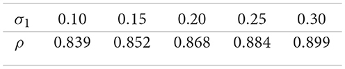
Response to Brownian volatility σ₁.

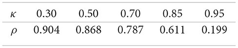
Response to risk–aversion κ.

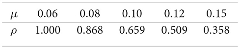
Response to expected return μ.

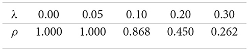
Response to jump scale λ.

5.3 Discussion of computational results

The computational experiments provide important insights into the comparative statics of the optimal portfolio fraction ρ in the jump–uncertain setting, highlighting how different market and preference parameters shape investment behavior. First, the results show that as the Brownian volatility σ₁ increases, the optimal allocation ρ to the risk–free asset rises monotonically. This pattern reflects the natural precautionary response to higher diffusion risk: Investors reduce exposure to the risky asset and seek safety in the risk–free asset, consistent with the negative coefficient of (κ − 1) in Equation 39. This finding underlines the stabilizing role of the risk–free asset in portfolios when market uncertainty is driven by continuous volatility. Second, the risk–aversion parameter κ exerts a powerful influence on the portfolio rule. For highly risk–averse investors (small κ), ρ is large, meaning that most wealth is allocated to the risk–free asset. As κ increases, reflecting weaker risk aversion and greater willingness to tolerate variability in returns, ρ declines, and wealth is shifted toward the risky asset. This comparative static emphasizes the theoretical consistency of the model with classical portfolio theory. Third, the effect of the expected return μ is particularly striking: As μ rises, ρ decreases sharply, shifting wealth into the risky asset. This is intuitive since higher expected reward offsets risk, encouraging more aggressive investment. Notably, when μ is low, the no–shorting constraint binds and the model projects ρ to one, implying a complete allocation to the risk–free asset. This binding case illustrates how constraints can dominate investor preferences when returns are insufficient to justify risky exposure. Finally, the V–jump intensity λ captures discontinuous risks that amplify downside exposure. The numerical results show that higher values of λ significantly increase ρ, reflecting investors' tendency to shield wealth from rare but severe shocks. For small λ, the projection again binds at ρ = 1, consistent with highly conservative behavior under jump risk, while for moderate to large λ, the optimal policy shifts markedly toward the risk–free asset. Overall, these findings demonstrate that the fraction ρ responds in economically consistent ways to both risk parameters and preference parameters. The comparative statics not only validate the theoretical formulation of the model but also provide practical guidance for portfolio selection, illustrating how investors adjust their allocation between risky and risk–free assets in response to changes in volatility, return, risk aversion, and jump exposure.

5.4 Summary

The computational findings indicate that the proposed model effectively replicates realistic investor decision-making across a range of market environments. The numerical simulations consistently exhibit comparative statics: The optimal proportion ρ allocated to the risk-free asset increases with both the Brownian volatility σ₁ and the jump intensity λ, signifying a heightened precautionary stance in response to elevated uncertainty. Conversely, ρ declines as the expected return on the risky asset μ rises, reflecting stronger incentives to assume risk for higher potential gains. Similarly, ρ decreases with the risk aversion coefficient κ, suggesting that less risk-averse investors allocate a smaller share to safe assets. Crucially, the value of ρ is determined solely by investor preferences and market parameters and remains independent of current wealth levels. This confirms the persistence of the constant-proportion investment rule under CRRA preferences, even in the presence of jump risk. Collectively, these outcomes substantiate the reliability and economic relevance of the proposed framework, emphasizing its practical effectiveness in guiding portfolio decisions under both continuous and jump-driven sources of uncertainty.

6 Conclusion

This study develops a unified framework for optimal portfolio selection in jump–uncertain stochastic markets, making both theoretical and computational contributions. On the theoretical side, we establish the existence and uniqueness of solutions to jump–uncertain stochastic differential equations, thereby extending the results of Chirima et al. [25], who studied the case without jumps in an uncertain–stochastic setting, and complementing the work of Chen and Liu [24], who proved an existence and uniqueness theorem in a Liu–uncertain framework without jumps. In addition, we provide a rigorous proof of the principle of optimality for jump–uncertain stochastic control problems. This result extends the work of Chirima et al. [3], who considered uncertain–stochastic systems without jumps, and generalizes the dynamic programming foundation developed by Chen and Liu [24], thereby reinforcing the link between dynamic programming and the maximum principle under both continuous and discontinuous uncertainty.

From a computational perspective, our analysis demonstrates that the framework captures realistic investor behavior across diverse market conditions. The numerical experiments reveal consistent comparative statics: The optimal fraction ρ invested in the risk–free asset increases with Brownian volatility σ₁ and jump intensity λ, reflecting stronger precautionary allocation under heightened uncertainty, while ρ decreases with the expected risky return μ and the risk–aversion parameter κ, indicating greater exposure to risk when expected returns rise or when investors are less risk–averse. Importantly, ρ depends only on preferences and market parameters, and not on current wealth, thereby confirming that the constant–proportion property of CRRA preferences persists in jump–uncertain settings.

Taken together, these findings underscore the robustness, tractability, and economic relevance of the proposed model. The result that the optimal fraction of wealth allocated to the risk-free asset remains independent of total wealth is a direct consequence of the constant–proportion investment rule under CRRA utility, which holds even in the presence of both Brownian and jump uncertainty. This outcome aligns with classical results in jump–diffusion models, notably those of Øksendal and Sulem [8], who demonstrated the same independence property. Similar conclusions were reached by Zhu [17] and Chirima et al. [3], further reinforcing the generality of this principle. More broadly, by integrating existence and uniqueness theory, the dynamic programming principle, and computational validation, this study offers a mathematically rigorous and practically applicable framework for portfolio optimization in markets subject to both continuous and discontinuous sources of risk.

Data availability statement

The raw data supporting the conclusions of this article will be made available by the authors, without undue reservation.

Author contributions

CH: Writing – original draft, Writing – review & editing, Conceptualization, Investigation. EC: Supervision, Writing – review & editing. CK: Supervision, Writing – review & editing. MM: Supervision, Writing – review & editing.

Funding

The author(s) declare that no financial support was received for the research and/or publication of this article.

Conflict of interest

The authors declare that the research was conducted in the absence of any commercial or financial relationships that could be construed as a potential conflict of interest.

Generative AI statement

The author(s) declare that no Gen AI was used in the creation of this manuscript.

Any alternative text (alt text) provided alongside figures in this article has been generated by Frontiers with the support of artificial intelligence and reasonable efforts have been made to ensure accuracy, including review by the authors wherever possible. If you identify any issues, please contact us.

Publisher's note

All claims expressed in this article are solely those of the authors and do not necessarily represent those of their affiliated organizations, or those of the publisher, the editors and the reviewers. Any product that may be evaluated in this article, or claim that may be made by its manufacturer, is not guaranteed or endorsed by the publisher.

References

1. Bellman R. Dynamic Programming. Princeton, NJ: Princeton University Press. (1957).

Google Scholar

2. Pontryagin LS, Boltyanskii VG, Gamkrelidze RV, Mishchenko EF. The Mathematical Theory of Optimal Processes. New York: Interscience Publishers. (1962).

Google Scholar

3. Chirima J, Matenda FR, Chikodza E, Sibanda M. Dynamic programming principle for optimal control of uncertain random differential equations and its application to optimal portfolio selection. Rev Busin Econo Stud. (2024) 12:74–85. doi: 10.26794/2308-944X-2024-12-3-74-85

Crossref Full Text | Google Scholar

4. Kushner HJ. On the Hamilton–Jacobi–Bellman equation for optimal stochastic control. J Math Anal Appl. (1965) 11:56–74.

Google Scholar

5. Fleming WH, Rishel RW. Deterministic and Stochastic Optimal Control. New York: Springer. (1975).

Google Scholar

6. Liu B. Uncertainty Theory. Berlin: Springer. (2010). doi: 10.1007/978-3-642-13959-8

Crossref Full Text | Google Scholar

7. Yong J, Zhou XY. Stochastic controls: Hamiltonian systems and HJB equations. In: Applications of Mathematics. New York: Springer. (1999).

Google Scholar

8. Øksendal B, Sulem A. Applied Stochastic Control of Jump Diffusions. 2nd ed. Berlin: Springer (2005).

Google Scholar

9. Peng S. A general stochastic maximum principle for optimal control problems. SIAM J Cont Optimizat. (1990) 28:966–79. doi: 10.1137/0328054

Crossref Full Text | Google Scholar

10. Ge X, Zhu Y. A necessary condition of optimality for uncertain optimal control problem. Fuzzy Opt Deci Making. (2013) 12:41–51. doi: 10.1007/s10700-012-9147-4

Crossref Full Text | Google Scholar

11. Chikodza E, Hlahla CK. Necessary Condition for Optimal Control of Uncertain Stochastic Systems. Singapore: Contemporary Mathematics, Universal Wiser Publisher (2025).

Google Scholar

12. Framstad NC, Øksendal B, Sulem A. Sufficient stochastic maximum principle for the optimal control of jump diffusions and applications to finance. J Optimizat Theory Appl. (2004) 121:77–98. doi: 10.1023/B:JOTA.0000026132.62934.96

Crossref Full Text | Google Scholar

13. Seba E. Oil Settles up 7% as Israel, Iran Trade Air Strikes (2025). Available online at: https://www.reuters.com/world/china/oil-prices-jump-more-than-4-after-israel-strikes-iran-2025-06-13 (Accessed July 06, 2025).

Google Scholar

14. Stephenson A. Oil Prices Up Nearly 3 Percent as Israel-Iran Conflict Escalates, US Response Remains Uncertain (2025). Available online at: https://www.reuters.com/business/energy/oil-falls-investors-weigh-chance-us-intervention-iran-israel-conflict-2025-06-19/?utm_source (Accessed July 06, 2025).

Google Scholar

15. Bousso R. Israel-Iran War Highlights Mideast's Declining Influence on Oil Prices (2025). Available online at: https://www.reuters.com/markets/commodities/israel-iran-war-highlights-mideasts-declining-influence-oil-prices-2025-06-25 (Accessed July 06, 2025).

Google Scholar

16. Liu B. Uncertainty Theory, 2nd ed. Berlin: Springer. (2007).

Google Scholar

17. Zhu Y. Uncertain optimal control with application to a portfolio selection model. Cybern Syst. (2010) 41:535–47. doi: 10.1080/01969722.2010.511552

Crossref Full Text | Google Scholar

18. Deng L, Zhu Y. Uncertain optimal control with jump. Comp Sci Inform Syst. (2012) 9:1453–68. doi: 10.2298/CSIS120225049D

Crossref Full Text | Google Scholar

19. Zhu Y. Uncertain Optimal Control. Cham: Springer Uncertainty Research. (2019).

Google Scholar

20. Fei W. Optimal control of uncertain stochastic systems with Markovian switching and its applications to portfolio decisions. Cybern Syst. (2014) 45:69–88. doi: 10.1080/01969722.2014.862445

Crossref Full Text | Google Scholar

21. Fei W. On existence and uniqueness of solutions to uncertain backwards stochastic differential equations. J Chin Univers. (2014) 29:55–66. doi: 10.1007/s11766-014-3048-y

PubMed Abstract | Crossref Full Text | Google Scholar

22. Markowitz H. Portfolio selection. J Finance. (1952) 7:77–91. doi: 10.1111/j.1540-6261.1952.tb01525.x

Crossref Full Text | Google Scholar

23. Merton RC. Optimum consumption and portfolio rules in a continuous-time model. J Econ Theory. (1971) 3:373–413. doi: 10.1016/0022-0531(71)90038-X

Crossref Full Text | Google Scholar

24. Chen X, Liu B. Existence and uniqueness theorem for uncertain differential equations. Fuzzy Optimiz Deci Making. (2010) 9:69–81. doi: 10.1007/s10700-010-9073-2

Crossref Full Text | Google Scholar

25. Chirima J, Chikodza E, Hove-Musekwa SD. Numerical Methods for first order uncertain stochastic differential equations. Int J Mathem Operat Res. (2020) 16:1–23. doi: 10.1504/IJMOR.2020.104679

PubMed Abstract | Crossref Full Text | Google Scholar

26. Hou Y. Subadditivity of chance measure. J Uncert Analy Appl. (2014) 2:14. doi: 10.1186/2195-5468-2-14

PubMed Abstract | Crossref Full Text | Google Scholar

27. Liu Y. Uncertain random variables: a mixture of uncertainty and randomness. Soft Comp. (2013) 17:625–34. doi: 10.1007/s00500-012-0935-0

Crossref Full Text | Google Scholar

28. Liu B. Uncertainty Theory, 5th ed. Beijing: Uncertainty Theory Laboratories. (2019).

PubMed Abstract | Google Scholar

29. Wu C, Yang L, Zhang C. Uncertain stochastic optimal control with jump and its application in a portfolio game. MDPI. (2022). 14. doi: 10.3390/sym14091885

Crossref Full Text | Google Scholar

30. Barles G, Imbert C. Second-order elliptic integro-differential equations: viscosity solutions' theory revisited. Ann I H Poincaré – AN. (2008) 25:567–85. doi: 10.1016/j.anihpc.2007.02.007

Crossref Full Text | Google Scholar

31. Kao EPC. An Introduction to Stochastic Processes. Belmont, CA: Wadsworth Publishing Company. (1997).

Google Scholar