Bootstrap confidence intervals of process capability indices Cpy and CNpmk using different methods of estimation for Frechet distribution

Process capability analysis is the statistical evaluation of process capability to examine how well it meets or exceeds the customers satisfaction. In present work, we are intended to evaluate two critical metrics for process quality assessment, C_py and C_Npmk for asymmetric Frechet distribution using different classical estimation methods namely: maximum likelihood, least squares, weighted least squares, Cramer-von-Mises, Anderson-Darling, right-tail Anderson-Darling, along Bayesian estimation using reference and Jeffreys priors. Furthermore, Monte Carlo simulations are conducted for comparative analysis of aforementioned estimation methods, using mean squared error and width of bootstrap confidence intervals. Comparative analysis demonstrates that Bayesian estimation using reference prior consistently producing smaller coefficient of mean squared errors and reduced width of bootstrap intervals for small to moderately large sample sizes. Moreover, the real data analysis is also validating the advantages of Bayesian estimations for process capability analysis.

1 Introduction

Statistical process control (SPC) is crucial for quality control in the highly competitive manufacturing industry. Process capability analysis is a vital component of SPC quality improvement programs. An essential part of SPC quality improvement initiatives is process capability analysis. Manufacturing process capabilities can be evaluated quantitatively and intuitively with the help of process capability indices (PCIs). These indices help identify areas for improvement and show how well a process meets customer needs. Over capability analysis, a process is evaluated using statistical methods to see whether it fulfills a set of customers preset specifications or not. Suppliers and manufacturers employ such measures to ensure that their finished products are of excellent quality and have the least amount of discrepancies. Capability indices are the most commonly used techniques for capability analysis. A PCI quantifies how well the process meets customer expectations.

Several PCIs have been suggested to quantify process performance. The readers may refer to Kane [1], addressed two often used indices: C_p and C_pk, Chan et al. [2] and Pearn et al. [3] devised two more advanced indices: C_pm and C_pmk. Choi and Owen [4] provided thorough comparisons of C_p, C_pk, C_pm, and C_pmk. Boyles [5] introduced PCI with asymmetric tolerance for C_pk, C_pm, and C_pmk. Many statisticians and quality researchers, including Kane [1], Chan et al. [2], Chou et al. [6], Pearn et al. [3], and Pearn and Chen [7], have discussed and analyzed point estimation and interval estimation of various indices.

The efficacy of these indicators is dependent on the process following a normal distribution [8–10]. However, the presence of various noise elements might occasionally result in abnormal manufacturing processes [11]. If the assumption is not met, these basic indices are not reliable [12–16]. For non-normal processes, the normality-based classical PCI may produce unreliable and misleading interpretations [17]. Pearn and Chen [18], Tong and Chen [19], and Senvar and Kahraman [17] all studied non-normal distributions. Still, we were unable to depend on one method that functions efficiently in all situations [11]. Furthermore, for various non-normal distributions, it is also claimed that each method performed differently [10]. Thus, for statisticians and practitioners, evaluating various PCIs under non-normal distributions is a crucial research topic. The widespread usage of PCIs in manufacturing requires a thorough analysis of proposed structures of PCIs in the literature using different estimating techniques and distributions.A PCI evaluates the amount of variation process experiences in relation to specification limitations. Point and interval estimations are often emphasized while analyzing PCIs. However, there is a possibility that point estimate will not conclude a realistic assessment of a process' capabilities and confidence intervals (CIs) are considered more useful in determining the variability of an estimate [20]. Hsiang and Taguchi [21] initiated the first move toward constructing CIs for the PCI. Since then, various methods for constructing CIs have been developed. One of these methods is bootstraping, which is unconstrained by distributional assumptions and makes complex inferences in simplified manners. In reality, insufficient or limited data is evaluated using a basic re-sampling method owing to time and budgetary restrictions. Franklin and Wasserman [22] initially used the bootstrap approach to evaluate the PCI-C_pk. Recently, significant advances have been made in the literature about bootstrap CIs and how they behave for processes in absence of normality assumption. Some studies in this regard include Kashif et al. [23], Rao et al. [24, 25], Peng [26], Dey and Saha [27, 28], Dey et al., [29], Saha et al. [30, 31], and Weber et al. [32].

Most statistical studies rely on one of two estimating categories: Bayesian or frequentist. PCIs for both normal and non-normal processes were developed using Bayesian and classical perspectives. Several statisticians, including Chan et al. [2], Cheng and Spiring [33], and Shiau et al. [34, 35], have justified and emphasized the advantages of the Bayesian method. Ramos et al. [36] provided a brief comparison of conventional and Bayesian estimation methods.

In present work, we are intended to develop PCIs named C_py and C_Npmk for Frechet distribution (FD) utilizing different classical methods provided in Ramos et al. [36] listed as, maximum likelihood, least square, Cramer-von-Mises and Anderson-Darling. Additionally, we are using weighted least square, right-tail Anderson-Darling estimators and Bayesian estimators using reference prior along Jeffrey prior for evaluation of PCIs.

The FD is a special case of the generalized extreme value distribution, used to model the maximum of large numbers of independent positive random variables. FD is equivalent to the inverse exponential distribution for the scale parameter β = 1; it is the inverse gamma distribution when β < 1 and for β = 2; it is the inverse Rayleigh distribution. The FD may be utilized in reliability analysis, especially when examining the quality characteristic of fatigue lifespan (the marketing life expectancy of pharmaceutical, automobile radiators, textile fatigue, and electron tubes, among other devices and variables). It provides flexible models for non-normal and asymmetric quality characteristics. Most suited to right-skewed characteristics where small values are most likely but rare extreme values exist. The probability density function (PDF), cumulative distribution function (CDF) and quantile function (QF) are given by

$\begin{array}{ll}f\left(x\mid \alpha ,\beta \right)=\left(\frac{\alpha }{\beta }\right){\left(\frac{\beta }{x}\right)}^{\alpha +1}exp\left[-{\left(\beta /x\right)}^{\alpha }\right];x,\alpha ,\beta >0& (1.1)\end{array}$

$\begin{array}{ll}F\left(x\mid \alpha ,\beta \right)=exp\left[-{\left(\beta /x\right)}^{\alpha }\right]& (1.2)\end{array}$

$\begin{array}{ll}Q\left({\text{γ}}_{\text{i}}\mid \alpha ,\beta \right)=\beta \left[-{\left(log\left({\text{γ}}_{\text{i}}\right)\right)}^{-\frac{1}{\alpha }}\right]& (1.3)\end{array}$

Kanwal and Abbas [37] evaluated PCIs S_pmk and C_s for FD. Kanwal and Abbas [38] provided comparative analysis of quantile based control charts for FD. It is important to note that while the quality characteristic X specifically follows FD, no effort has been taken to investigate PCIs particularly C_py and C_Npmk. The research aims to bridge the gap. Our objective is to provide recommendations for selecting the most effective PCI estimation technique. It is hoped this study will benefit quality engineers, management professionals, and statisticians. In continuation to the introductory section, the remainder of the article is structured as follows. Section 2 comprises of introduction to PCI C_py and PCI C_Npmk. In Section 3 sensitivity analysis is performed, Section 4 presents several classical estimation methods for C_py and C_Npmk whereas bootstrap confidence intervals (BCIs) are covered in Section 5. Section 6 includes a simulation study to evaluate the estimators' effectiveness in estimating C_py and C_Npmk in terms of mean squared error (MSE), coefficient of skewness (${\sqrt{\beta }}_1$), coefficient of kurtosis (β₂), and BCIs width. Section 7 analyzes the real-life data set as an illustration. Finally, the findings of the present study are shown in Section 8.

2 PCIs C_py and C_Npmk

The detail of PCIs C_py and C_Npmk is given below.

2.1 PCI C_py

A generalized PCI C_py has been proposed by Maiti et al. [39]. It includes continuous and discrete random variables, both normal and non-normal, and is either directly or indirectly associated with most PCIs in literature. It can be defined as:

$\begin{array}{ll}{C}_{py}=\frac{F\left(USL\right)-F\left(LSL\right)}{F\left(UDL\right)-F\left(LDL\right)}=\frac{p}{p_0}& (2.1)\end{array}$

where p is the process output, p₀ is the desired output, LDL and UDL denotes the lower and upper desirable limits, and USL and LSL are upper and lower specifications respectively. Where, LDL = μ−3σ and UDL = μ+3σ. PCI C_py may be expressed as (p/0.9973) for process following a normal distribution. The C_py for FD quality characteristic can be expressed as

$\begin{array}{ll}{C}_{py}=\frac{1}{p_0}\left[exp\left[-{\left(\beta /USL\right)}^{\alpha }\right]-exp\left[-{\left(\beta /LSL\right)}^{\alpha }\right]\right]& (2.2)\end{array}$

2.2 PCI C_Npmk

Vannman [40] combined these four indices C_p, C_pk, C_pm and C_pmk into one super-structure, defined as

$\begin{array}{l}{C}_p\left(u,v\right)=\frac{d-u|\mu -m|}{3\sqrt{{\sigma }^2+v{\left(\mu -T\right)}^2}},u,v\ge 0\end{array}$

where d = (USL − LSL)/2 and m = (USL + LSL)/2. In particular, we have, C_p(0, 0) = C_p, C_p(1, 0) = C_pk, C_p(0, 1) = C_pm and C_p(1, 1) = C_pmk. These indices have been developed when underlying distribution is normal. Later, Chen and Pearn [16] generalized Vannman [40] work and developed a new quantile-based PCI index CNp (u, v) for any underlying distribution, defined as

$\begin{array}{l}{C}_{Np}\left(u,v\right)=\frac{d-u|M-m|}{3\sqrt{{\left(\frac{F_{99.865}-F_{0.135}}{6}\right)}^2+v{\left(M-T\right)}^2}},\end{array}$

where F_α is the α-th percentile, M is the median. Whereas, median M for is a more robust measure skewed distributions than the process mean μ. Setting (u, v)= (1, 1) leads to C_Npmk, for any distribution, given as

$\begin{array}{l}{C}_{Npmk}=min\left\{C_{NpmkU},C_{NpmkL}\right\}\end{array}$

where

$\begin{array}{l}{C}_{NpmkU}=\frac{USL-M}{3\sqrt{{\left(\frac{Q\left({\gamma }_3\mid \alpha ,\beta \right)-Q\left({\gamma }_1\mid \alpha ,\beta \right)}{6}\right)}^2+{\left(Q\left({\gamma }_2\mid \alpha ,\beta \right)-T\right)}^2}}\end{array}$

and

$\begin{array}{l}{C}_{NpmkL}=\frac{M-LSL}{3\sqrt{{\left(\frac{Q\left({\gamma }_3\mid \alpha ,\beta \right)-Q\left({\gamma }_1\mid \alpha ,\beta \right)}{6}\right)}^2+{\left(Q\left({\gamma }_2\mid \alpha ,\beta \right)-T\right)}^2}}.\end{array}$

where, γ_i − th are quantiles of the two parameter FD with parameters (α, β). The C_Npmk for FD quality characteristic can be written as

$\begin{array}{ll}{C}_{Npmk}=\frac{min\left(USL-M,M-LSL\right)}{3\sqrt{{\left(\frac{\beta \left(-log{\left(\frac{3}{4}\right)}^{-\left(\frac{1}{\alpha }\right)}-log{\left(\frac{1}{4}\right)}^{-\left(\frac{1}{\alpha }\right)}\right)}{6}\right)}^2+{\left(M-T\right)}^2}}& (2.3)\end{array}$

3 Sensitivity analysis

For a given PCI, the net sensitivity (NS) analysis for distribution function is proposed by Maiti et al. [39], and is defined as

$\begin{array}{l}NS=\frac{1}{p_0}{\displaystyle \underset{ϵ\to 0}{lim}}\left[\frac{\left\{F\left(U\right)-F\left(L\right)\right\}-\left\{F\left(U-ϵ\right)-F\left(L-ϵ\right)\right\}}{ϵ}\right]\\ =\frac{f\left(U\right)-f\left(L\right)}{p_0},\end{array}$

If the NS values are low (in absolute) with respect to the PCI, the distribution is less sensitive and more robust. However, if the NS values are positive, the considered distribution is more sensitive (or less robust) at USL than at LSL; if the NS values are negative, the converse is true. The unit of measurement for the NS values is defectives per million (dpm). The NS values for the following distributions are presented in Table 1. It is apparent from Table 1 that overall FD is more robust as compare to Weibul and log-logistic distribution and Figure 1 shows that Weibull, log-logistic and FD all are less sensitive (or more robust) at USL for the considered values of (L; U) = (1;4) and p₀ = 0.95, respectively.

Table 1

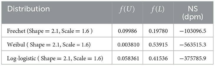
Table 1. Sensitivity analysis for FD.

Figure 1

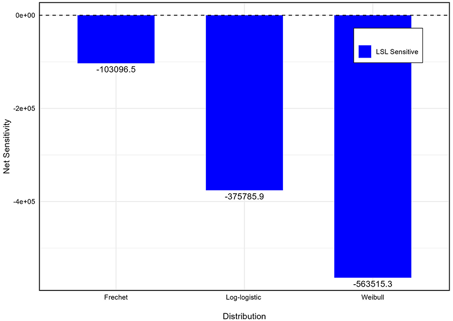
Figure 1. Sensitivity for FD.

4 Different methods of estimation for C_py and C_Npmk

Here, we describe eight different estimators, namely, maximum likelihood estimator (MLE), ordinary least square estimator(LSE) and weighted least squares estimator (WLSE), Cramer-von-Mises estimator (CVME), Anderson-Darling estimator (ADE), and right tail Anderson-Darling estimator (RTADE), Bayesian estimator under reference prior (BERP), and Jeffrey prior (BEJP) to find out the estimates of the parameters α and β for FD and the corresponding estimators of C_py and C_Npmk respectively. The non-linear equations can be solved by using nleqslv package which is available in the R-software [41].

4.1 Maximum likelihood estimator

Let x₁, x₂, …, x_n be a random sample of size n taken from Equation 1.1. Then the log-likelihood function is

$\begin{array}{l}l=nlog\left(\alpha \right)-n\alpha log\left(\beta \right)-\left(\alpha +1\right){\displaystyle \sum _{i=1}^n}log\left(x_i\right)-{\displaystyle \sum _{i=1}^n}{\left(\frac{\beta }{x_i}\right)}^{\alpha }\end{array}$

The partial derivatives are

$\begin{array}{ll}\frac{\partial l}{\partial \alpha }=\frac{n}{\alpha }+nlog\left(\beta \right)-{\displaystyle \sum _{i=1}^n}log\left(x_i\right)-{\displaystyle \sum _{i=1}^n}{\left(\frac{\beta }{x_i}\right)}^{\alpha }log\left(\frac{\beta }{x_i}\right)=0& (4.1)\end{array}$

$\begin{array}{ll}\frac{\partial l}{\partial \beta }=\frac{n\alpha }{\beta }-\left(\frac{\alpha }{\beta }\right){\displaystyle \sum _{i=1}^n}{\left(\frac{\beta }{x_i}\right)}^{\alpha }=0& (4.2)\end{array}$

The solutions to these equations do not result in closed form for MLEs. However, these equations are solved simultaneously using a numerical approach. Substituting the MLEs in Equations 2.2, 2.3, we can get the estimators of C_py and C_Npmk as

$\begin{array}{ll}{Ĉ}_{py}^{MLE}=\frac{1}{p_0}\left[exp\left\{-{\left({\widehat{\beta }}_{MLE}/USL\right)}^{{\widehat{\alpha }}_{MLE}}\right\}-exp\left\{-{\left({\widehat{\beta }}_{MLE}/LSL\right)}^{{\widehat{\alpha }}_{MLE}}\right\}\right]& (4.3)\end{array}$

$\begin{array}{ll}{Ĉ}_{Npmk}^{MLE}=\frac{min\left(USL-M,M-LSL\right)}{3\sqrt{{\left(\frac{\begin{array}{c}{\widehat{\beta }}_{MLE}(-log{\left(\frac{3}{4}\right)}^{-\left(\frac{1}{{\widehat{\alpha }}_{MLE}}\right)}\\ -log{\left(\frac{1}{4}\right)}^{-\left(\frac{1}{{\widehat{\alpha }}_{MLE}}\right)})\end{array}}{6}\right)}^2+{\left(M-T\right)}^2}}.& (4.4)\end{array}$

4.1.1 Ordinary and weighted least squares estimator

Swain et al. [42] proposed a least squares approach to minimize the distance in Johnson's translation system. Suppose F(x_(i:n)|α, β) denotes the CDF of ordered random variables x₁ ≤ x₂ ≤ ... ≤ x_n of size n from a distribution function F(^.|α, β). The least squares estimators of ${\widehat{\alpha }}_{LSE}$ and ${\widehat{\beta }}_{LSE}$ can be obtained by minimizing the function

$\begin{array}{ll}S\left(\alpha ,\beta \right)={\displaystyle \sum _{i=1}^n}{\left[F\left(x_{\left(i:n\right)}|\alpha ,\beta \right)-\frac{i}{n+1}\right]}^2,& (4.5)\end{array}$

differentiating with respect to α and β. The estimators can be obtained by solving the following

$\begin{array}{ll}{\displaystyle \sum _{i=1}^n}\left[F\left(x_{\left(i\right)}|\alpha ,\beta \right)-\frac{i}{n+1}\right]{\xi }_1\left(x_i|\alpha ,\beta \right)=0,& (4.6)\end{array}$

$\begin{array}{ll}{\displaystyle \sum _{i=1}^n}\left[F\left(x_{\left(i\right)}|\alpha ,\beta \right)-\frac{i}{n+1}\right]{\xi }_2\left(x_i|\alpha ,\beta \right)=0,& (4.7)\end{array}$

where

$\begin{array}{ll}{\xi }_1\left(x_i|\alpha ,\beta \right)=-exp{\left\{-\left(\frac{\beta }{x_i}\right)\right\}}^{\alpha }{\left(\frac{\beta }{x_i}\right)}^{\alpha }log\left(\frac{\beta }{x_i}\right)=0,& (4.8)\end{array}$

and

$\begin{array}{ll}{\xi }_2\left(x_i|\alpha ,\beta \right)=-\frac{exp{\left\{-\left(\frac{\beta }{x_i}\right)\right\}}^{\alpha }\alpha {\left(\frac{\beta }{x_i}\right)}^{\alpha -1}}{x_i}=0.& (4.9)\end{array}$

Similarly, the weighted least squares estimator of ${\widehat{\alpha }}_{WLSE}$ and ${\widehat{\beta }}_{WLSE}$ can be obtained by minimizing the function by Erto and Genesis [43].

$\begin{array}{ll}W\left(\alpha ,\beta \right)={\displaystyle \sum _{i=1}^n}\frac{{\left(n+1\right)}^2\left(n+2\right)}{i\left(n-i+1\right)}{\left[F\left(x_{\left(i:n\right)}|\alpha ,\beta \right)-\frac{i}{n+1}\right]}^2=0,& (4.10)\end{array}$

WLSEs can be obtained by solving the following

$\begin{array}{ll}{\displaystyle \sum _{i=1}^n}\frac{{\left(n+1\right)}^2\left(n+2\right)}{i\left(n-i+1\right)}\left[F\left(x_{\left(i:n\right)}|\alpha ,\beta \right)-\frac{i}{n+1}\right]{\xi }_1\left(x_i|\alpha ,\beta \right)=0,& (4.11)\end{array}$

$\begin{array}{ll}{\displaystyle \sum _{i=1}^n}\frac{{\left(n+1\right)}^2\left(n+2\right)}{i\left(n-i+1\right)}\left[F\left(x_{\left(i:n\right)}|\alpha ,\beta \right)-\frac{i}{n+1}\right]{\xi }_2\left(x_i|\alpha ,\beta \right)=0.& (4.12)\end{array}$

Where ξ₁(x_i|α, β) and ξ₂(x_i|α, β) are shown in Equations 4.8, 4.9. The least squares and weighted least squares estimators of PCI-C_py for FD are

$\begin{array}{ll}{Ĉ}_{py}^{LSE}=\frac{1}{p_0}\left[exp\left\{-{\left({\widehat{\beta }}_{LSE}/USL\right)}^{{\widehat{\alpha }}_{LSE}}\right\}-exp\left\{-{\left({\widehat{\beta }}_{LSE}/LSL\right)}^{{\widehat{\alpha }}_{LSE}}\right\}\right]& (4.13)\end{array}$

$\begin{array}{l}{Ĉ}_{py}^{WLSE}=\frac{1}{p_0}[exp\left\{-{\left({\widehat{\beta }}_{WLSE}/USL\right)}^{{\widehat{\alpha }}_{WLSE}}\right\}\\ -exp\left\{-{\left({\widehat{\beta }}_{WLSE}/LSL\right)}^{{\widehat{\alpha }}_{WLSE}}\right\}]& (4.14)\end{array}$

Similarly, the least squares and weighted least squares estimators of PCI-C_Npmk for FD are

$\begin{array}{ll}{Ĉ}_{Npmk}^{LSE}=\frac{min\left(USL-M,M-LSL\right)}{3\sqrt{{\left(\frac{{\widehat{\beta }}_{LSE}\left(-log{\left(\frac{3}{4}\right)}^{-\left(\frac{1}{{\widehat{\alpha }}_{LSE}}\right)}-log{\left(\frac{1}{4}\right)}^{-\left(\frac{1}{{\widehat{\alpha }}_{LSE}}\right)}\right)}{6}\right)}^2+{\left(M-T\right)}^2}}& (4.15)\end{array}$

$\begin{array}{ll}{Ĉ}_{Npmk}^{WLSE}=\frac{min\left(USL-M,M-LSL\right)}{3\sqrt{{\left(\frac{\begin{array}{c}{\widehat{\beta }}_{WLSE}(-log{\left(\frac{3}{4}\right)}^{-\left(\frac{1}{{\widehat{\alpha }}_{WLSE}}\right)}\\ -log{\left(\frac{1}{4}\right)}^{-\left(\frac{1}{{\widehat{\alpha }}_{WLSE}}\right)})\end{array}}{6}\right)}^2+{\left(M-T\right)}^2}}.& (4.16)\end{array}$

4.1.2 Cramer-von-Mises estimator

The Cramer-von-Mises test was proposed by Cramer [44] and von-Mises [45], which measures the distance between empirical distribution function and CDF of assumed model. Moreover, Boos [46] studied its properties, which can be expressed as

$\begin{array}{ll}CVM\left(\alpha ,\beta \right)=\frac{1}{12n}+{\displaystyle \sum _{i=1}^n}{\left[F\left(x_{\left(i:n\right)}|\alpha ,\beta \right)-\frac{2i-1}{2n}\right]}^2,& (4.17)\end{array}$

The Cramer-von-Mises estimator of ${\widehat{\alpha }}_{CVME}$ and ${\widehat{\beta }}_{CVME}$ can be incurred by solving the following

$\begin{array}{ll}{\displaystyle \sum _{i=1}^n}\left[F\left(x_{\left(i:n\right)}|\alpha ,\beta \right)-\frac{2i-1}{2n}\right]{\xi }_1\left(x_i|\alpha ,\beta \right)=0,& (4.18)\end{array}$

$\begin{array}{ll}{\displaystyle \sum _{i=1}^n}\left[F\left(x_{\left(i:n\right)}|\alpha ,\beta \right)-\frac{2i-1}{2n}\right]{\xi }_2\left(x_i|\alpha ,\beta \right)=0.& (4.19)\end{array}$

Where ξ₁(x_i|α, β) and ξ₂(x_i|α, β) are mentioned in Equations 4.8, 4.9. The corresponding estimators of PCIs-C_py and C_Npmk are

$\begin{array}{l}{Ĉ}_{py}^{CVME}=\frac{1}{p_0}[exp\left\{-{\left({\widehat{\beta }}_{CVME}/USL\right)}^{{\widehat{\alpha }}_{CVME}}\right\}\\ -exp\left\{-{\left({\widehat{\beta }}_{CVME}/LSL\right)}^{{\widehat{\alpha }}_{CVME}}\right\}]& (4.20)\end{array}$

$\begin{array}{ll}{Ĉ}_{Npmk}^{CVME}=\frac{min\left(USL-M,M-LSL\right)}{3\sqrt{{\left(\frac{\begin{array}{c}{\widehat{\beta }}_{CVME}(-log{\left(\frac{3}{4}\right)}^{-\left(\frac{1}{{\widehat{\alpha }}_{CVME}}\right)}\\ -log{\left(\frac{1}{4}\right)}^{-\left(\frac{1}{{\widehat{\alpha }}_{CVME}}\right)})\end{array}}{6}\right)}^2+{\left(M-T\right)}^2}}.& (4.21)\end{array}$

4.1.3 Anderson-Darling estimator

Anderson-Darling [47] statistic belong to the class of quadratic empirical distribution function [48]. The Anderson-Darling test (ADT) converges rapidly toward the asymptote [49], which is

$\begin{array}{l}ADT\left(\alpha ,\beta \right)=-n-\frac{1}{n}{\displaystyle \sum _{i=1}^n}\left(2i-1\right)[log\left(F\left(x_{\left(i\right)}|\alpha ,\beta \right)\right)\\ +log\left(1-\left(F\left(x_{\left(1-i+n\right)}|\alpha ,\beta \right)\right)\right)]& (4.22)\end{array}$

The Anderson-Darling estimator (ADE), ${\widehat{\alpha }}_{ADE}$ and ${\widehat{\beta }}_{ADE}$ can also be obtained by solving the following non-linear equations

$\begin{array}{ll}{\displaystyle \sum _{i=1}^n}\left(2i-1\right)\left[\frac{\begin{array}{c}-\text{exp}\left\{-{\left(\frac{\beta }{x_i}\right)}^{\alpha }\right\}log\left(\frac{\beta }{x_{\left(i\right)}}\right){\left(\frac{\beta }{x_{\left(i\right)}}\right)}^{\alpha }\\ +\frac{exp\left\{-{\left(\frac{\beta }{x_{\left(1-i+n\right)}}\right)}^{\alpha }\right\}log\left(\frac{\beta }{\left(1-i+n\right)}\right){\left(\frac{\beta }{x_{\left(1-i+n\right)}}\right)}^{\alpha }}{1-exp\left\{-{\left(\frac{\beta }{x_{\left(1-i+n\right)}}\right)}^{\alpha }\right\}}\end{array}}{\text{exp}\left\{-{\left(\frac{\beta }{x_i}\right)}^{\alpha }\right\}+log\left[1-exp\left\{-{\left(\frac{\beta }{x_{\left(1-i+n\right)}}\right)}^{\alpha }\right\}\right]}\right]& (4.23)\end{array}$

$\begin{array}{ll}{\displaystyle \sum _{i=1}^n}\left(2i-1\right)\left[\frac{\begin{array}{c}-\frac{\text{exp}\left\{-{\left(\frac{\beta }{x_i}\right)}^{\alpha }\right\}\alpha {\left(\frac{\beta }{x_{\left(i\right)}}\right)}^{-1+\alpha }}{x_i}\\ +\frac{exp\left\{-{\left(\frac{\beta }{x_{\left(1-i+n\right)}}\right)}^{\alpha }\right\}\alpha {\left(\frac{\beta }{x_{\left(1-i+n\right)}}\right)}^{-1+\alpha }}{\left(1-exp\left\{-{\left(\frac{\beta }{x_{\left(1-i+n\right)}}\right)}^{\alpha }\right\}\right)x_{\left(1-i+n\right)}}\end{array}}{\text{exp}\left\{-{\left(\frac{\beta }{x_i}\right)}^{\alpha }\right\}+log\left(1-exp\left\{-{\left(\frac{\beta }{x_{\left(1-i+n\right)}}\right)}^{\alpha }\right\}\right)}\right]& (4.24)\end{array}$

The right tail Anderson-Darling estimator, ${\widehat{\alpha }}_{RTADE}$ and ${\widehat{\beta }}_{RTADE}$ are obtained by minimizing with respect to α and β, the function

$\begin{array}{l}RTADE\left(\alpha ,\beta \right)=\frac{n}{2}-2{\displaystyle \sum _{i=1}^n}F\left(x_{\left(i\right)}|\alpha ,\beta \right)-\frac{1}{n}{\displaystyle \sum _{i=1}^n}\left(2i-1\right)\\ log\left(1-\left(F\left(x_{\left(1-i+n\right)}|\alpha ,\beta \right)\right)\right),& (4.25)\end{array}$

These estimators can also be obtained by solving the following non-linear equations

$\begin{array}{l}-{\displaystyle \underset{i=1}{\stackrel{n}{2\sum }}}\frac{exp\left\{-{\left(\frac{\beta }{x_{\left(i\right)}}\right)}^{\alpha }\right\}log\left(\frac{\beta }{x_{\left(i\right)}}\right){\left(\frac{\beta }{x_{\left(i\right)}}\right)}^{\alpha }}{1-exp\left\{-{\left(\frac{\beta }{x_{\left(i\right)}}\right)}^{\alpha }\right\}}\\ -{\displaystyle \underset{i=1}{\stackrel{n}{\frac{1}{n}\sum }}}\frac{exp\left\{-{\left(\frac{\beta }{x_{\left(i\right)}}\right)}^{\alpha }-{\left(\frac{\beta }{x_{\left(1-i+n\right)}}\right)}^{\alpha }\right\}log\left(\frac{\beta }{x_{\left(1-i+n\right)}}\right){\left(\frac{\beta }{x_{\left(1-i+n\right)}}\right)}^{\alpha }}{{\left(1-exp\left\{-{\left(\frac{\beta }{x_{\left(i\right)}}\right)}^{\alpha }\right\}\right)}^2}\\ =0,& (4.26)\end{array}$

$\begin{array}{l}-2{\displaystyle \sum _{i=1}^n}\frac{exp\left\{-{\left(\frac{\beta }{x_{\left(i\right)}}\right)}^{\alpha }\right\}\alpha {\left(\frac{\beta }{x_{\left(i\right)}}\right)}^{-1+\alpha }}{\left(1-exp\left\{-{\left(\frac{\beta }{x_{\left(i\right)}}\right)}^{\alpha }\right\}\right)x_{\left(i\right)}}\\ -\frac{1}{n}{\displaystyle \sum _{i=1}^n}\frac{exp\left\{-{\left(\frac{\beta }{x_{\left(i\right)}}\right)}^{\alpha }-{\left(\frac{\beta }{x_{\left(1-i+n\right)}}\right)}^{\alpha }\right\}\alpha {\left(\frac{\beta }{x_{\left(1-i+n\right)}}\right)}^{-1+\alpha }}{{\left(1-exp\left\{-{\left(\frac{\beta }{x_{\left(i\right)}}\right)}^{\alpha }\right\}\right)}^2{x}_{\left(1-i+n\right)}}\\ =0.& (4.27)\end{array}$

The ADE and RTADE of PCI C_py for FD are

$\begin{array}{l}{Ĉ}_{py}^{ADE}=\frac{1}{p_0}[exp\left\{-{\left({\widehat{\beta }}_{ADE}/USL\right)}^{{\widehat{\alpha }}_{ADE}}\right\}\\ -exp\left\{-{\left({\widehat{\beta }}_{ADE}/LSL\right)}^{{\widehat{\alpha }}_{ADE}}\right\}]& (4.28)\end{array}$

$\begin{array}{l}{Ĉ}_{py}^{RTADE}=\frac{1}{p_0}[exp\left\{-{\left({\widehat{\beta }}_{RTADE}/USL\right)}^{{\widehat{\alpha }}_{RTADE}}\right\}\\ -exp\left\{-{\left({\widehat{\beta }}_{RTADE}/LSL\right)}^{{\widehat{\alpha }}_{RTADE}}\right\}]& (4.29)\end{array}$

Similarly, the corresponding ADE and RTADE of PCI C_Npmk for FD are

$\begin{array}{ll}{Ĉ}_{Npmk}^{ADE}=\frac{min\left(USL-M,M-LSL\right)}{3\sqrt{{\left(\frac{\begin{array}{c}{\widehat{\beta }}_{ADE}(-log{\left(\frac{3}{4}\right)}^{-\left(\frac{1}{{\widehat{\alpha }}_{ADE}}\right)}\\ -log{\left(\frac{1}{4}\right)}^{-\left(\frac{1}{{\widehat{\alpha }}_{ADE}}\right)})\end{array}}{6}\right)}^2+{\left(M-T\right)}^2}}& (4.30)\end{array}$

$\begin{array}{ll}{Ĉ}_{Npmk}^{RTADE}=\frac{min\left(USL-M,M-LSL\right)}{3\sqrt{{\left(\frac{\begin{array}{c}{\widehat{\beta }}_{RTADE}(-log{\left(\frac{3}{4}\right)}^{-\left(\frac{1}{{\widehat{\alpha }}_{RTADE}}\right)}\\ -log{\left(\frac{1}{4}\right)}^{-\left(\frac{1}{{\widehat{\alpha }}_{RTADE}}\right)})\end{array}}{6}\right)}^2+{\left(M-T\right)}^2}}.& (4.31)\end{array}$

4.2 Bayesian estimator

This section considers the BERP and BEJP for estimation of unknown parameters of the FD. Abbas and Tang [50] derived Jeffrey's and reference priors for FD, which are as follows:

$\begin{array}{l}{\pi }_J\left(\alpha ,\beta \right)\propto \sqrt{\left|I\left(\alpha ,\beta \right)\right|}\propto \frac{1}{\beta }\\ {\pi }_R\left(\alpha ,\beta \right)\propto \sqrt{\left|I\left(\alpha ,\beta \right)\right|}\propto \frac{1}{\alpha \beta }\end{array}$

The joint posterior distributions using Jeffrey's and reference prior can be written as

$\begin{array}{ll}{\pi }_J\left(\alpha ,\beta \mid x\right)=\frac{{\alpha }^n{\beta }^{n\alpha -1}{\displaystyle {\prod }_{i=1}^n}{x}_i^{-\left(\alpha +1\right)}exp\left[-{\displaystyle {\sum }_{i=1}^n}{\left(\beta /x_i\right)}^{\alpha }\right]}{\begin{array}{c}{\displaystyle {\int }_0^{\infty }}{\displaystyle {\int }_0^{\infty }}{\alpha }^n{\beta }^{n\alpha -1}{\displaystyle {\prod }_{i=1}^n}{x}_i^{-\left(\alpha +1\right)}\\ exp\left[-{\displaystyle {\sum }_{i=1}^n}{\left(\beta /x_i\right)}^{\alpha }\right]d\alpha d\beta \end{array}}.& (4.32)\end{array}$

$\begin{array}{ll}{\pi }_R\left(\alpha ,\beta \mid x\right)=\frac{\begin{array}{c}{\alpha }^{n-1}{\beta }^{n\alpha -1}{\displaystyle {\prod }_{i=1}^n}{x}_i^{-\left(\alpha +1\right)}\\ exp\left[-{\displaystyle {\sum }_{i=1}^n}{\left(\beta /x_i\right)}^{\alpha }\right]\end{array}}{\begin{array}{c}{\displaystyle {\int }_0^{\infty }}{\displaystyle {\int }_0^{\infty }}{\alpha }^{n-1}{\beta }^{n\alpha -1}{\displaystyle {\prod }_{i=1}^n}{x}_i^{-\left(\alpha +1\right)}\\ exp\left[-{\displaystyle {\sum }_{i=1}^n}{\left(\beta /x_i\right)}^{\alpha }\right]d\alpha d\beta \end{array}}.& (4.33)\end{array}$

The Bayesian estimators of model parameters employing squared error loss function are obtained using Laplace approximation. Which is accessible through the LearnBayes package [51]. The BERP and BEJP of PCI-C_py are given as

$\begin{array}{l}{Ĉ}_{py}^{BERP}=\frac{1}{p_0}[exp\left\{-{\left({\widehat{\beta }}_{BERP}/USL\right)}_{BERP}^{\widehat{\alpha }}\right\}\\ -exp\left\{-{\left({\widehat{\beta }}_{BERP}/LSL\right)}^{{\widehat{\alpha }}_{BERP}}\right\}]& (4.34)\end{array}$

$\begin{array}{l}{Ĉ}_{py}^{BEJP}=\frac{1}{p_0}[exp\left\{-{\left({\widehat{\beta }}_{BEJP}/USL\right)}_{BEJP}^{\widehat{\alpha }}\right\}\\ -exp\left\{-{\left({\widehat{\beta }}_{BEJP}/LSL\right)}^{{\widehat{\alpha }}_{BEJP}}\right\}]& (4.35)\end{array}$

Similarly, the corresponding BERP and BEJP of PCI C_Npmk for FD are

$\begin{array}{ll}{Ĉ}_{Npmk}^{BERP}=\frac{min\left(USL-M,M-LSL\right)}{3\sqrt{{\left(\frac{\begin{array}{c}{\widehat{\beta }}_{BERP}(-log{\left(\frac{3}{4}\right)}^{-\left(\frac{1}{{\widehat{\alpha }}_{BERP}}\right)}\\ -log{\left(\frac{1}{4}\right)}^{-\left(\frac{1}{{\widehat{\alpha }}_{BERP}}\right)})\end{array}}{6}\right)}^2+{\left(M-T\right)}^2}}& (4.36)\end{array}$

$\begin{array}{ll}{Ĉ}_{Npmk}^{BEJP}=\frac{min\left(USL-M,M-LSL\right)}{3\sqrt{{\left(\frac{\begin{array}{c}{\widehat{\beta }}_{BEJP}(-log{\left(\frac{3}{4}\right)}^{-\left(\frac{1}{{\widehat{\alpha }}_{BEJP}}\right)}\\ -log{\left(\frac{1}{4}\right)}^{-\left(\frac{1}{{\widehat{\alpha }}_{BEJP}}\right)})\end{array}}{6}\right)}^2+{\left(M-T\right)}^2}}.& (4.37)\end{array}$

5 BCIs for C_py and C_Npmk

Franklin and Wasserman [22] developed the bootstrap approach, which is typically employed to obtain the empirical distribution of different PCIs. We evaluated standard BCIs for C_py and C_Npmk. The basic steps for bootstrapping are as follows:

• A random sample (x₁, x₂, …, x_n) of size n, is drawn from FD(α, β), followed by n bootstrap samples (with replacement) taken from the original sample with a mass of 1/n at each. Classical and Bayesian estimates of $(\widehat{\alpha },\widehat{\beta })$ are obtained and then R-th bootstrap estimator are calculated for C_py & C_Npmk, i.e.,

$\begin{array}{l}{Ĉ}_{py}^{\left(R\right)}={Ĉ}_{py}\left(x_1,x_2,\cdots ,x_n\right)\&\\ {Ĉ}_{Npmk}^{\left(R\right)}={Ĉ}_{Npmk}\left(x_1,x_2,\cdots ,x_n\right)\\ \end{array}$

• A total of nⁿ re-samples exist, and for each sample, ${Ĉ}_{py}^{(R)}$ is obtained, resulting in a full bootstrapped distribution $\left\{{Ĉ}_{py}^{*(\mathcal{J})};\mathcal{J}=1(1)\mathcal{B}\right\}$ and is denoted by ${Ĉ}_{py}^{*(1)}\le {Ĉ}_{py}^{*(2)}\le \cdots \le {Ĉ}_{py}^{*(\mathcal{B})}$, and same process is done for ${Ĉ}_{Npmk}^{(R)}$.

6 Simulation study

The present section deals with the simulation experiment for performance assessments of the PCIs namely C_py and C_Npmk for FD based on aforementioned estimation methods. Different parametric combinations (α, β) = [(1, 3.5)(1, 2)(1, 4)(1.2, 2.2)] for C_py and (1, 2.5), (2.1, 1.6), [1.6, 2.1, (1.6,1.7)] for C_Npmk against sample size n = 10, 15, 20, 25, 30, 50 are evaluated and the LSL and USL are set as 1 and 4, respectively whereas, target value is 2.5 and p₀ = 0.95. For each design, 95% BCIs were evaluated, along the difference of both the upper and lower confidence bounds, referred as the average width, (${\sqrt{\beta }}_1$), (β₂), and MSE, to compare the results shown in Tables 2–5 for PCI C_py and Tables 6–9 for PCI C_Npmk with 10,000 replications using the R-software. Results are evaluated based on indices with reduced average width and minimum MSE.

Table 2

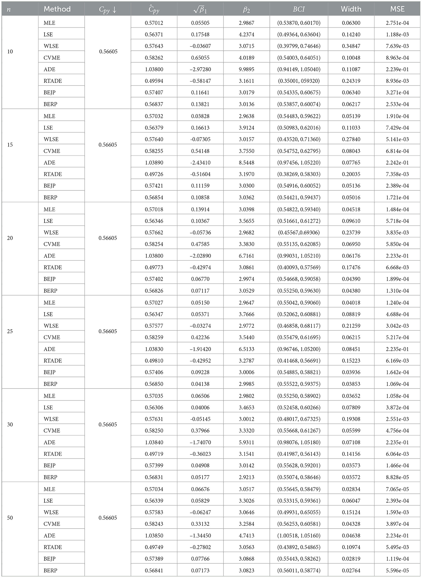
Table 2. Estimates of C_py when α = 1.2 and β = 2.2.

Table 3

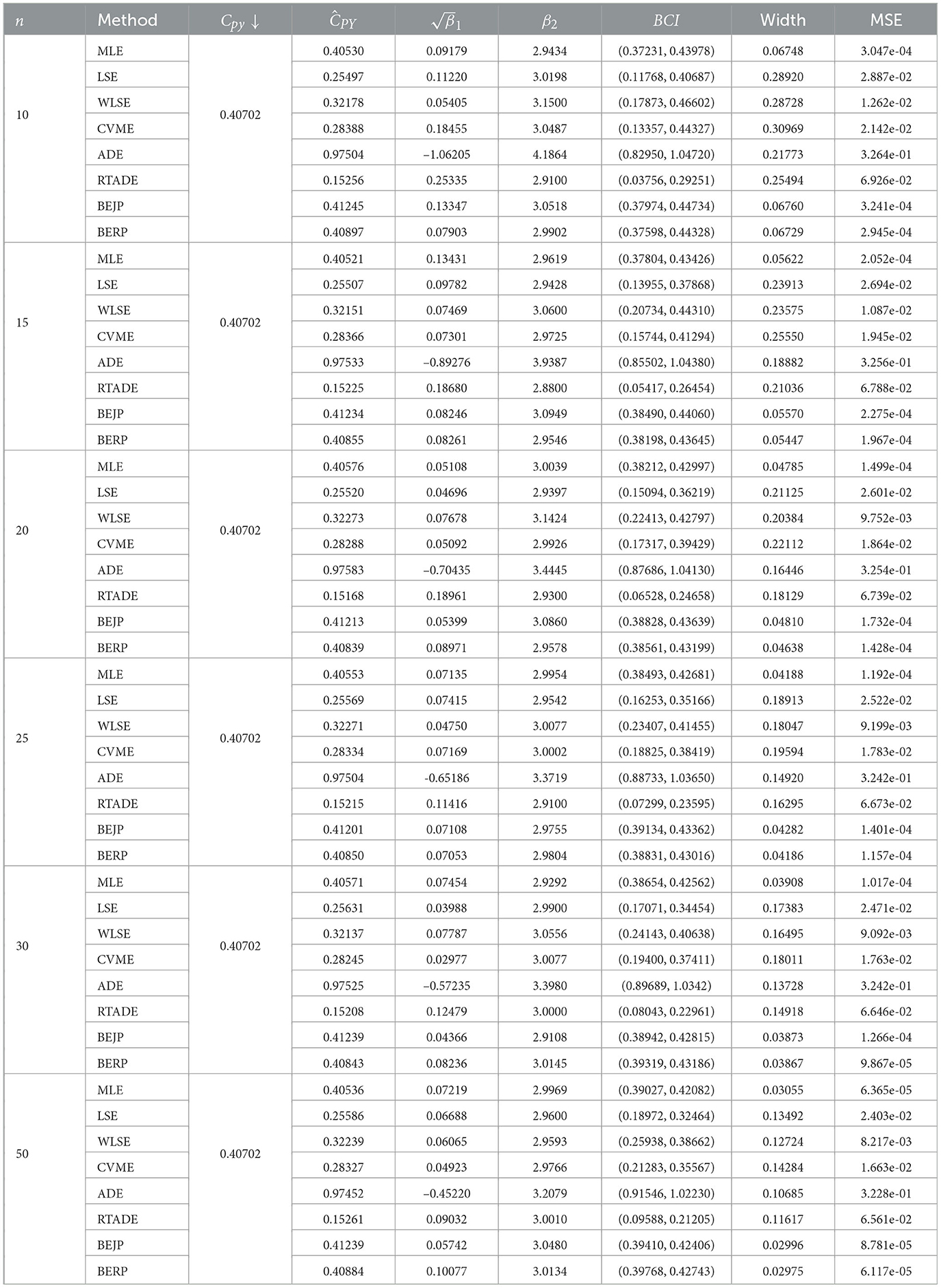
Table 3. Estimates of C_py when α = 1 and β = 3.5.

Table 4

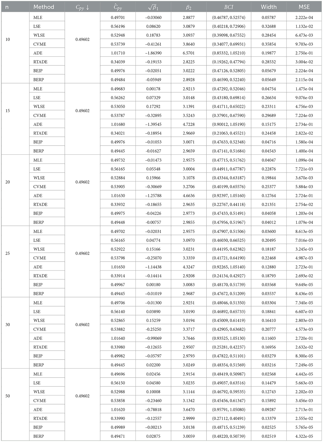
Table 4. Estimates of C_py when α = 1 and β = 2.

Table 5

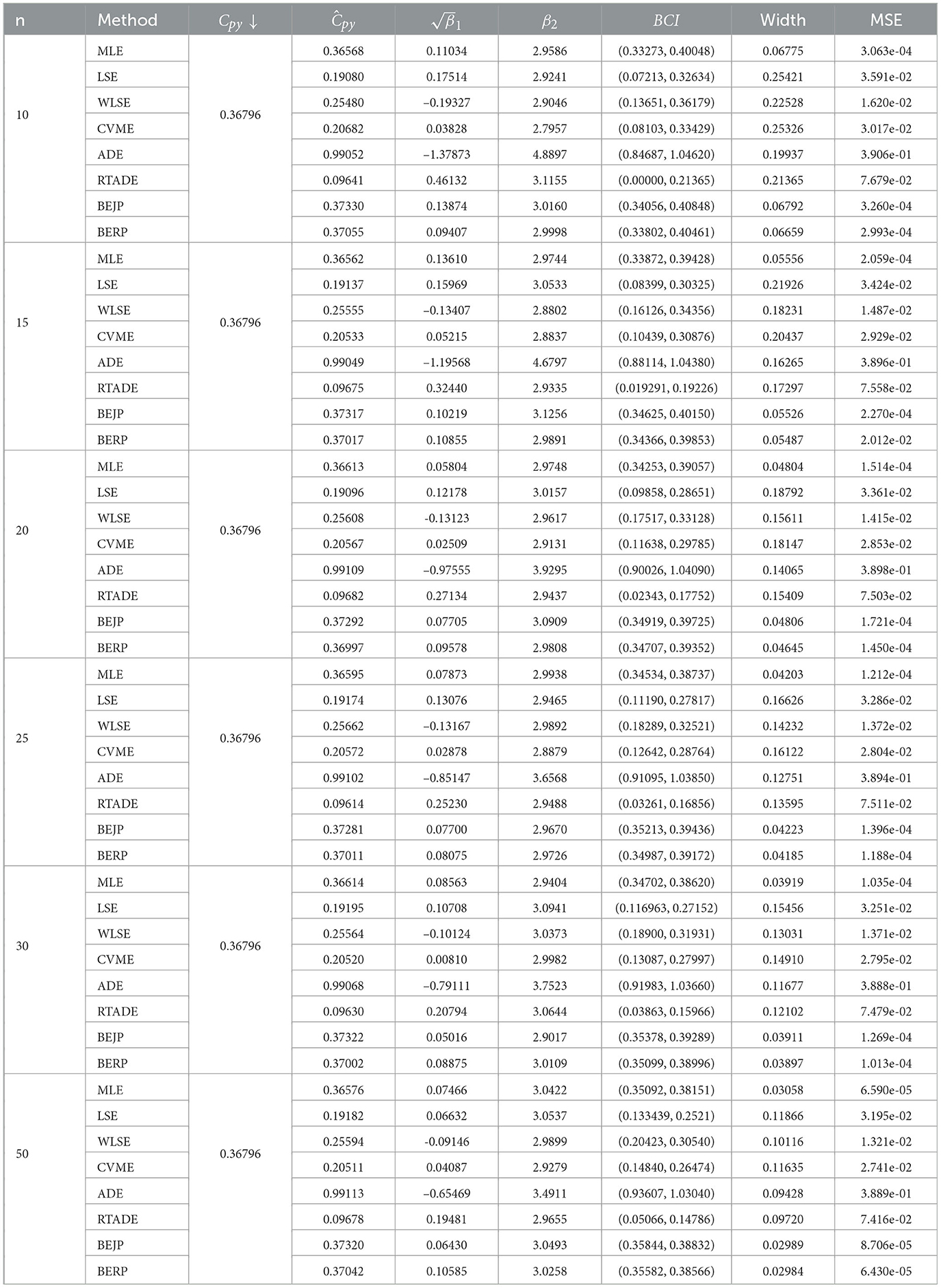
Table 5. Estimates for C_py when α = 1 and β = 4.

Table 6

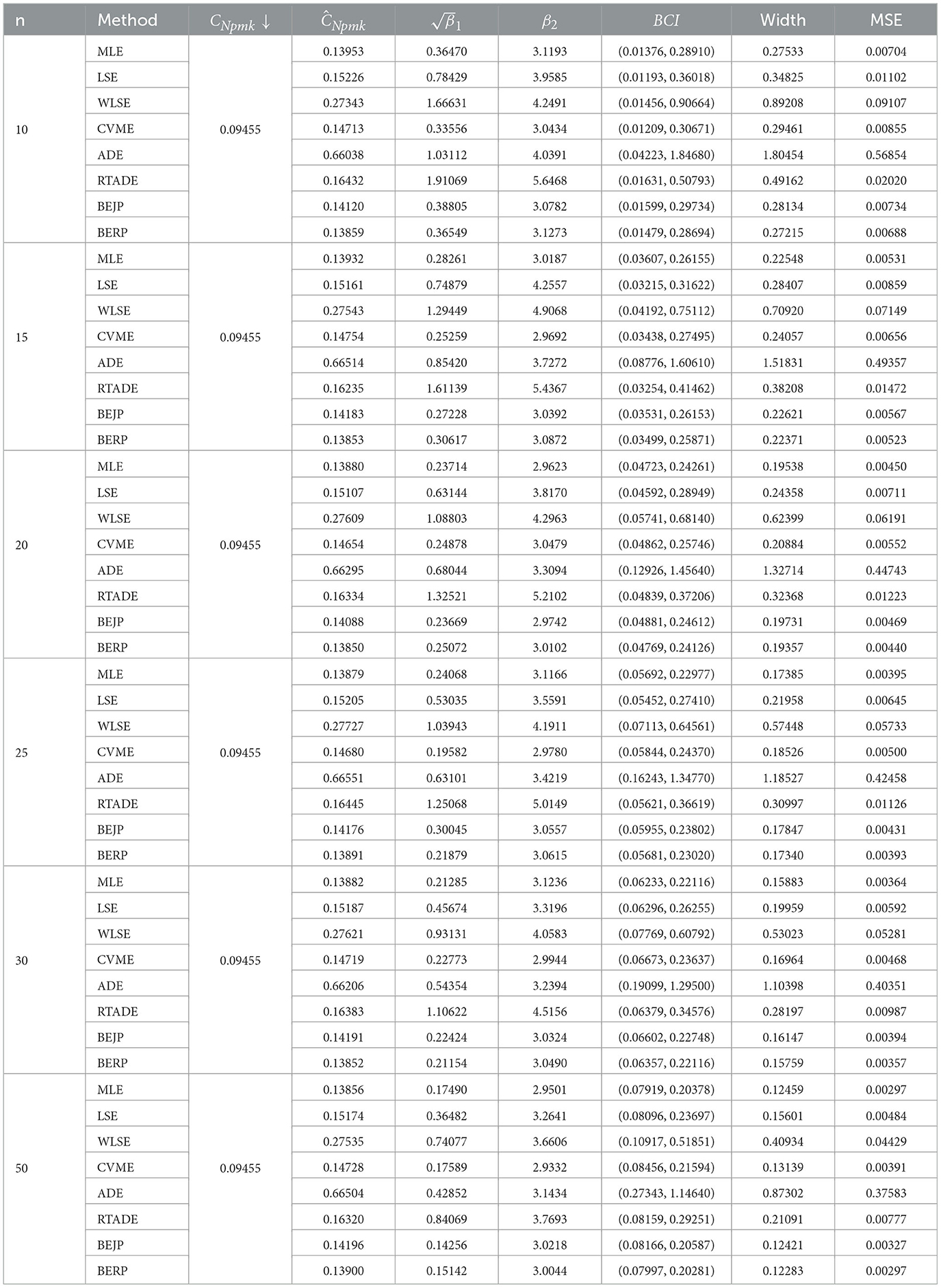
Table 6. Estimates of C_Npmk when α = 1 and β = 2.5.

Table 7

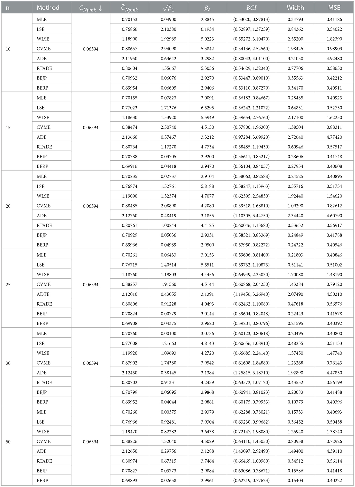
Table 7. Estimates of C_Npmk when α = 1.6 and β = 1.7.

Table 8

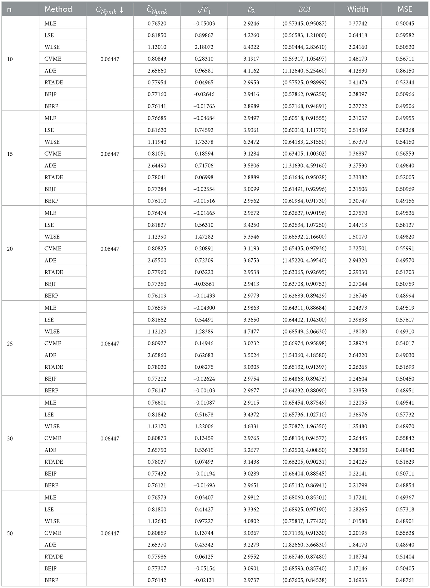
Table 8. Estimates of C_Npmk when α = 1.6 and β = 2.1.

Table 9

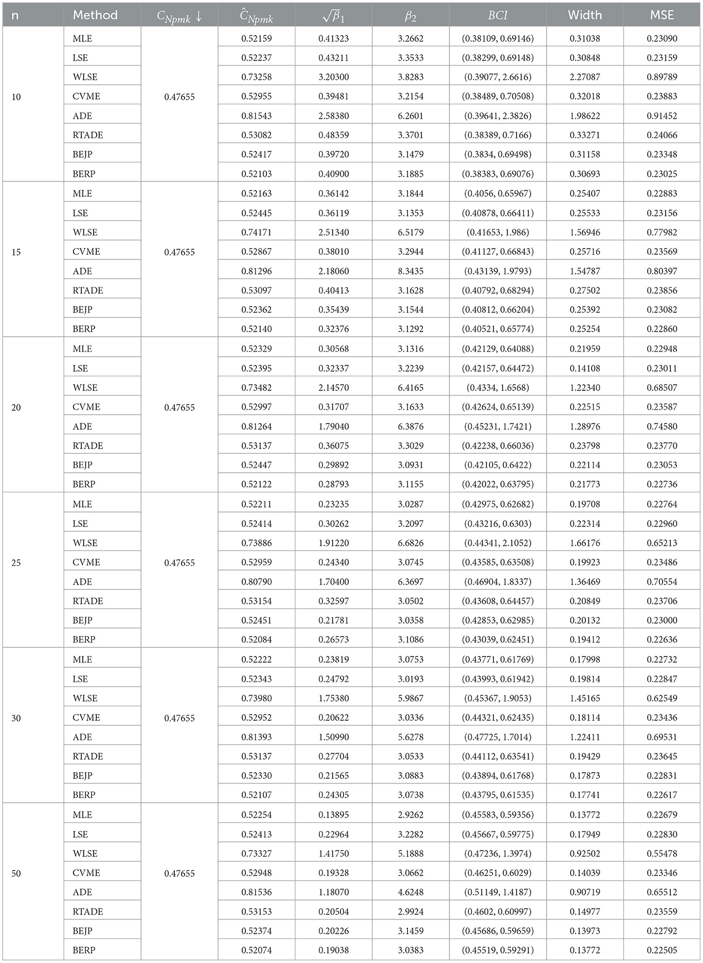
Table 9. Estimates of C_Npmk when α = 2.1 and β = 1.6.

The results presented in Tables 2–9, all demonstrate that with increase in sample size, both average width and MSE are reduced for all PCIs against all estimation methods, suggesting that a small sample size, n < 25 and moderately large (30, 50) sample produces better results.

If we look more closely, we can find that the BERP has minimum MSEs for small to moderate sample sizes when compared to MLE, LSE, WLSE, CVME, ADE, RTADE, and BEJP. Moreover, the MSE are least for BERP for both PCIs C_py and C_Npmk. Furthermore, in this investigation BERP outperformed other estimating methods by producing the least width of estimates for the configurations under consideration.

7 Real data illustration

This section examines the actual dataset comprising of the failure timings of 20 electric carts, as presented by Rao et al. [24], listed in Table 10. To evaluate the BCIs of PCIs the estimation methods ML, LS, WLS, CVM, AD, RTAD, BEJP, and BERP are utilized. Initially, we evaluate if the analyzed data set originates from a FD by examining the p-value of the Kolmogorov-Smirnov (KS) test, Anderson-Darling (AD) and Cramer-von Mises (CVM) test. The point estimates for the data set are α = 0.9070176, β = 5.2836813. The statistic along with p-values of corresponding goodness of fit test are summarized in Table 11 and complemented the analysis with graphical diagnostics, density and PP plots in Figure 2. Which are evident that this data set follows two parameter FD quite well. To estimate the PCIs, the USL and LSL, were set to 53.0 and 0.90 respectively and p₀ = 0.95. The mean of the data set, T = 26.95, is set as the target value. Table 12 shows the BCI widths of the PCIs C_py and C_Npmk based on the aforementioned estimation techniques for FD. It is clear from Table 12 that BERP has a narrow BCI than its counterparts. BERP is a more effective method for employing PCI interval estimations. For all PCIs, BERP outperformed MLE and BEJP and all aforementioned methods in terms of BCI width. The distribution shape of PCIs is approximately normal. This study suggests that BERP is more effective for examining observed PCIs.

Table 10

Table 10. Lifetime (in months) for failure of 20 electric carts.

Table 11

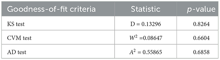
Table 11. The goodness-of-fit test for FD.

Figure 2

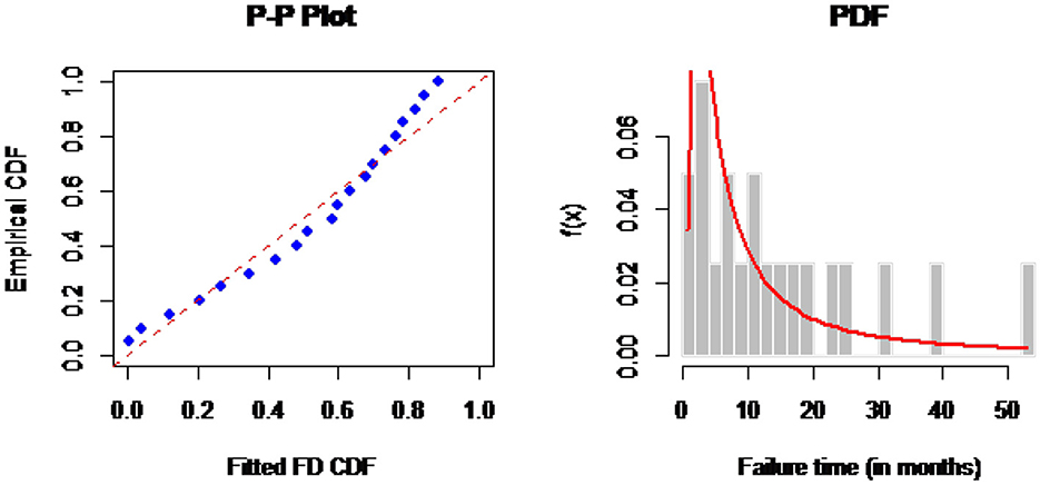
Figure 2. PP and density plots of FD.

Table 12

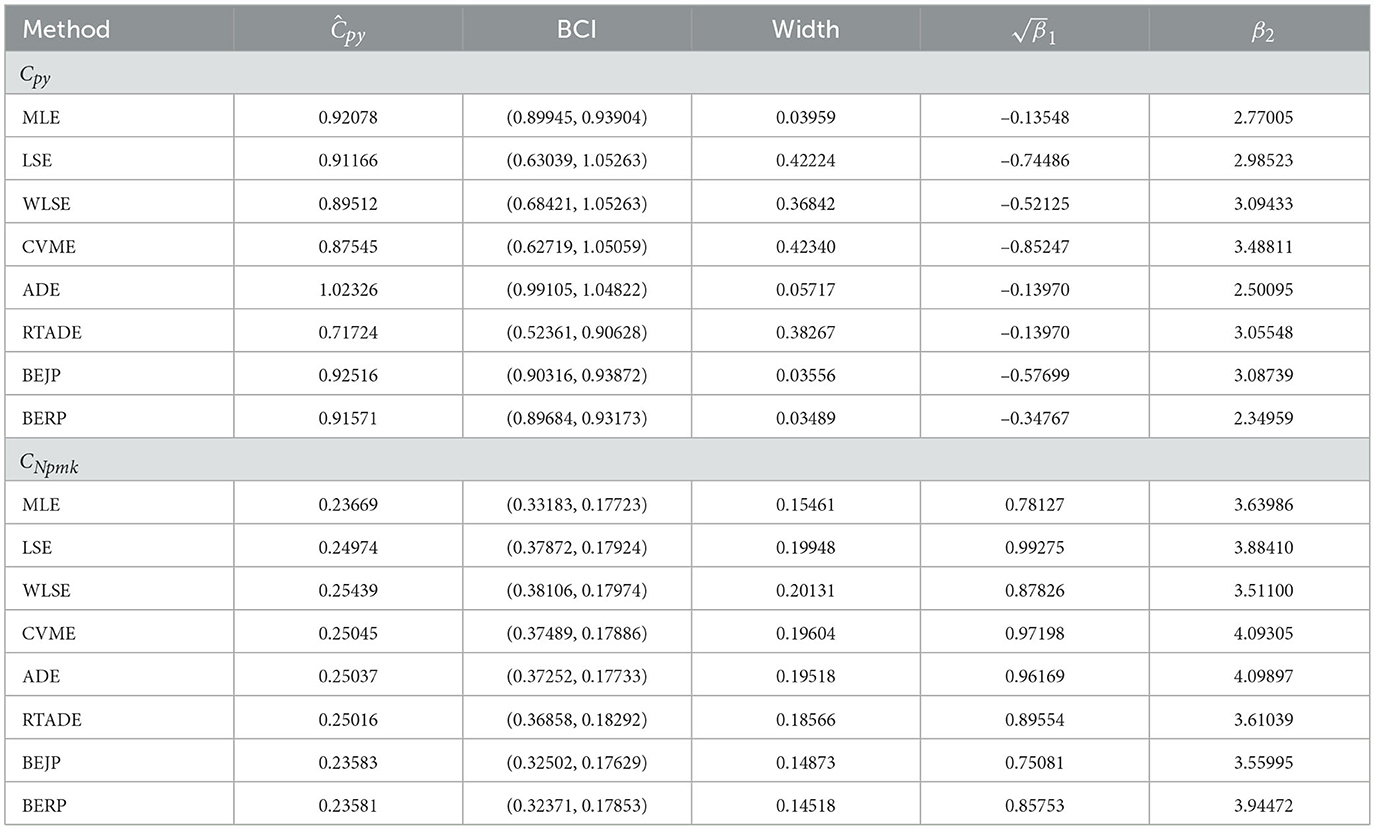
Table 12. Estimates of PCIs.

8 Conclusion

This article examines two PCIs: C_py and C_Npmk, using various estimating approaches for FD. In general, we used the MLE, LSE, WLSE, CVME, ADE, RTADE, BERP, and BEJP to produce estimates and BCIs for the aforementioned PCIs. Extensive simulation studies were conducted to compare these approaches with various small to moderately large sample sizes and parametric values. The average estimates for these PCIs, along with their coefficient of skewness, kurtosis, BCIs, and corresponding MSEs, have been acquired. The MSE of C_Npmk is significantly less than that of C_py. Furthermore, simulation findings indicated that BERP outperformed the other estimators for MSEs and the width of PCIs. The examination of the real data set validated this finding. This study aims to help engineering professionals and applied statisticians.

Data availability statement

The original contributions presented in the study are included in the article/supplementary material, further inquiries can be directed to the corresponding author.

Author contributions

TK: Formal analysis, Methodology, Software, Writing – original draft, Conceptualization. KA: Project administration, Supervision, Software, Writing – review & editing. MZ: Resources, Writing – review & editing. ZH: Writing – review & editing, Resources, Methodology.

Funding

The author(s) declare that no financial support was received for the research and/or publication of this article.

Conflict of interest

The authors declare that the research was conducted in the absence of any commercial or financial relationships that could be construed as a potential conflict of interest.

Generative AI statement

The author(s) declare that no Gen AI was used in the creation of this manuscript.

Any alternative text (alt text) provided alongside figures in this article has been generated by Frontiers with the support of artificial intelligence and reasonable efforts have been made to ensure accuracy, including review by the authors wherever possible. If you identify any issues, please contact us.

Publisher's note

All claims expressed in this article are solely those of the authors and do not necessarily represent those of their affiliated organizations, or those of the publisher, the editors and the reviewers. Any product that may be evaluated in this article, or claim that may be made by its manufacturer, is not guaranteed or endorsed by the publisher.

References

1. Kane VE. Process capability indices. J Quality Technol. (1986) 18:41–52. doi: 10.1080/00224065.1986.11978984

Crossref Full Text | Google Scholar

2. Chan LK, Cheng SW, Spiring FA. A new measure of process capability: CPM. J Quality Technol. (1988) 20:162–75. doi: 10.1080/00224065.1988.11979102

Crossref Full Text | Google Scholar

3. Pearn WL, Kotz S, Johnson NL. Distributional and inferential properties of process capability indices. J Quality Technol. (1992) 24:216–31. doi: 10.1080/00224065.1992.11979403

Crossref Full Text | Google Scholar

4. Choi BC, Owen DB. A study of a new process capably index. Commun Stat Theory Methods. (1990) 19:1231–45. doi: 10.1080/03610929008830258

Crossref Full Text | Google Scholar

5. Boyles RA. Process capability with asymmetric tolerances. Commun Stat Simul Comput. (1994) 23:615–35. doi: 10.1080/03610919408813190

Crossref Full Text | Google Scholar

6. Chou YM, Owen DB, Salvador A, Borrego A. Lower confidence limits on process capability indices. J Quality Technol. (1990) 22:223–9. doi: 10.1080/00224065.1990.11979242

Crossref Full Text | Google Scholar

7. Pearn WL, Chen KS, A. Bayesian-like estimator of CPK. Commun Stat Simul Comput. (1996) 25:321–9. doi: 10.1080/03610919608813316

Crossref Full Text | Google Scholar

8. Kashif M, Aslam M, Al-Marshadi AH, Jun CH. Capability indices for non-normal distribution using Ginis mean difference as measure of variability. IEEE Access. (2016) 4:7322–30. doi: 10.1109/ACCESS.2016.2620241

Crossref Full Text | Google Scholar

9. Panichkitkosolkul W. Confidence intervals for the process capability index CP based on confidence intervals for variance under non-normality. Malays J Mathem Sci. (2016) 10:101–15.

Google Scholar

10. Senvar O, Sennaroglu B. Comparing performances of clements, box-cox, Johnson methods with weibull distributions for assessing process capability. J Ind Eng Manag. (2016) 9:634–56. doi: 10.3926/jiem.1703

Crossref Full Text | Google Scholar

11. Piña-Monarrez MR, Ortiz-Yañez JF, Rodríguez-Borbón MI. Non-normal capability indices for the Weibull and lognormal distributions. Quality Reliab Eng Int. (2016) 32:1321–9. doi: 10.1002/qre.1832

Crossref Full Text | Google Scholar

12. Chan LK, Cheng SW, Spiring FA. The Robustness of the Process Capability Index CP to Departures From Normality. North Holland, Amsterdam: Statistical Theory and Data Analysis II (1988). p. 223–39.

Google Scholar

13. Gunter B. The use and abuse of CPK. Quality Progr. (1989) 22:86–7.

Google Scholar

14. English JR, Taylor GD. Process capability analysis - a robustness study. Int J Prod Res. (1993) 31:1621–35. doi: 10.1080/00207549308956813

Crossref Full Text | Google Scholar

15. Somerville SE, Montgomery DC. Process capability indices and non-normal distributions. Qual Eng. (1996) 9:305–16. doi: 10.1080/08982119608919047

Crossref Full Text | Google Scholar

16. Chen KS, Pearn WL. An application of non-normal process capability indices. Quality Reliab Eng Int. (1997) 13:355–60. doi: 10.1002/(SICI)1099-1638(199711/12)13:6<355::AID-QRE125>3.0.CO;2-V

Crossref Full Text | Google Scholar

17. Senvar O, Kahraman C. Type-2 fuzzy process capability indices for non-normal processes. J Intell Fuzzy Syst. (2014) 27:769–81. doi: 10.3233/IFS-131035

Crossref Full Text | Google Scholar

18. Pearn WL, Chen KS. Estimating process capability indices for non-normal pearsonian populations. Quality Reliab Eng Int. (1995) 11:386–8. doi: 10.1002/qre.4680110510

Crossref Full Text | Google Scholar

19. Tong LI, Chen JP. Lower confidence limits of process capability indices for non-normal process distributions. Int J Quality Reliab Manag. (1998) 15:907–19. doi: 10.1108/02656719810199006

Crossref Full Text | Google Scholar

20. Smithson M. Correct confidence intervals for various regression effect sizes and parameters: the importance of noncentral distributions in computing intervals. Educ Psychol Meas. (2001) 61:605–32. doi: 10.1177/00131640121971392

Crossref Full Text | Google Scholar

21. Hsiang TC, A. tutorial on quality control and assurance-the Taguchi methods. In: ASA Annual Meeting LA. (1985).

Google Scholar

22. Franklin LA, Gary W. Bootstrap confidence interval estimates of CPK: an introduction. Commun Stat Simul Comput. (1991) 20:231–42. doi: 10.1080/03610919108812950

Crossref Full Text | Google Scholar

23. Kashif M, Aslam M, Rao GS, AL-Marshadi AH, Jun CH. Bootstrap confidence intervals of the modified process capability index for Weibull distribution. Arabian J Sci Eng. (2017) 42:4565–73. doi: 10.1007/s13369-017-2562-7

Crossref Full Text | Google Scholar

24. Rao GS, Aslam M, Kantam RR. Bootstrap confidence intervals of C NPK for inverse Rayleigh and log-logistic distributions. J Stat Comput Simul. (2016) 86:862–73. doi: 10.1080/00949655.2015.1040799

Crossref Full Text | Google Scholar

25. Rao GS, Albassam M, Aslam M. Evaluation of bootstrap confidence intervals using a new non-normal process capability index. Symmetry. (2019) 11:484–92. doi: 10.3390/sym11040484

Crossref Full Text | Google Scholar

26. Peng C. Parametric lower confidence limits of quantile-based process capability indices. Quality Technol Quant Manag. (2010) 7:199–214. doi: 10.1080/16843703.2010.11673228

Crossref Full Text | Google Scholar

27. Dey S, Saha M, Maiti SS, Jun CH. Bootstrap confidence intervals of generalized process capability index CPYK for Lindley and power Lindley distributions. Commun Stat Simul Comput. (2018) 47:249–62. doi: 10.1080/03610918.2017.1280166

Crossref Full Text | Google Scholar

28. Dey S, Saha M. Bootstrap confidence intervals of generalized process capability index C PYK using different methods of estimation. J Appl Stat. (2019) 46:1843–69. doi: 10.1080/02664763.2019.1572721

Crossref Full Text | Google Scholar

29. Dey S, Saha M. Bootstrap confidence intervals of process capability index S PMK using different methods of estimation. J Stat Comput Simul. (2020) 90:28–50. doi: 10.1080/00949655.2019.1671980

Crossref Full Text | Google Scholar

30. Saha M, Dey S, Maiti SS. Parametric and non-parametric bootstrap confidence intervals of C NPK for exponential power distribution. J Ind Prod Eng. (2018) 35:160–9. doi: 10.1080/21681015.2018.1437793

Crossref Full Text | Google Scholar

31. Saha M, Dey S, Maiti SS. Bootstrap confidence intervals of C pTk for two parameter logistic exponential distribution with applications. Int J Syst Assur Eng Manag. (2019) 10:623–31. doi: 10.1007/s13198-019-00789-7

Crossref Full Text | Google Scholar

32. Weber S, Ressurreição T, Duarte C. Yield prediction with a new generalized process capability index applicable to non-normal data. IEEE Trans Comput-Aided Des Integr Circ Syst. (2015) 35:931–42. doi: 10.1109/TCAD.2015.2481865

Crossref Full Text | Google Scholar

33. Cheng SW, Spiring FA. Assessing process capability: a Bayesian approach. IIE Trans. (1989) 21:97–8. doi: 10.1080/07408178908966212

Crossref Full Text | Google Scholar

34. Shiau JJ, Chiang CT, Hung HN. A Bayesian procedure for process capability assessment. Quality Reliab Eng Int. (1999) 15:369–78. doi: 10.1002/(SICI)1099-1638(199909/10)15:5<369::AID-QRE262>3.0.CO;2-R

Crossref Full Text | Google Scholar

35. Shiau JJ, Hung HN, Chiang CT. A note on Bayesian estimation of process capability indices. Stat Probab Lett. (1999) 45:215–24. doi: 10.1016/S0167-7152(99)00061-9

Crossref Full Text | Google Scholar

36. Ramos PL, Louzada F, Ramos E, Dey S. The Frechet distribution: estimation and application-an overview. J Stat Manag Syst. (2020) 23:549–78. doi: 10.1080/09720510.2019.1645400

Crossref Full Text | Google Scholar

37. Kanwal T, Abbas K. Bootstrap confidence intervals of process capability indices SPMK, SPMKC and CS for Frechet distribution. Quality Reliab Eng Int. (2023) 39:2244–57. doi: 10.1002/qre.3333

Crossref Full Text | Google Scholar

38. Kanwal T, Abbas K. Comparative analysis of quantile-based control charts for Frechet distribution. Qual Eng. (2025) 2025:1–16. doi: 10.1080/08982112.2025.2543006

Crossref Full Text | Google Scholar

39. Maiti SS, Saha M, Nanda AK. On generalizing process capability indices. Quality Technol Quant Manag. (2010) 7:279–300. doi: 10.1080/16843703.2010.11673233

Crossref Full Text | Google Scholar

40. Vannman K. A Unified approach to capability indices. Statistica Sinika. (1995) 5:805–20.

Google Scholar

41. Dennis Jr JE, Schnabel RB. Numerical Methods for Unconstrained Optimization and Nonlinear Equations. Society for Industrial and Applied Mathematics. (1996). doi: 10.1137/1.9781611971200

Crossref Full Text | Google Scholar

42. Swain JJ, Venkatraman S, Wilson JR. Least-squares estimation of distribution functions in Johnson's translation system. J Stat Comput Simul. (1988) 29:271–97. doi: 10.1080/00949658808811068

Crossref Full Text | Google Scholar

43. Erto P. Genesis properties and identification of the inverse Weibull lifetime model. Statistica Appl. (1989) 1:117–28.

Google Scholar

44. Cramer H. On the composition of elementary errors: First paper: mathematical deductions. Scand Actuar J. (1928) 1928:13–74. doi: 10.1080/03461238.1928.10416862

Crossref Full Text | Google Scholar

45. Von Mises RE. Wahrscheinlichkeitsrechnung. Deuticke, Vienna.

Google Scholar

46. Boos DD. Minimum distance estimators for location and goodness of fit. J Am Stat Assoc. (1981) 76:663–70. doi: 10.1080/01621459.1981.10477701

Crossref Full Text | Google Scholar

47. Anderson TW, Darling DA. Asymptotic theory of certain" goodness of fit" criteria based on stochastic processes. Ann Mathem Stat. (1952) 1:193–212. doi: 10.1214/aoms/1177729437

Crossref Full Text | Google Scholar

48. Stephens MA. EDF statistics for goodness of fit and some comparisons. J Am Stat Assoc. (1974) 69:730–7. doi: 10.1080/01621459.1974.10480196

Crossref Full Text | Google Scholar

49. Pettitt AN. A two-sample Anderson-Darling rank statistic. Biometrika. (1976) 63:161–8. doi: 10.1093/biomet/63.1.161

Crossref Full Text | Google Scholar

50. Abbas K, Tang Y. Analysis of Frechet distribution using reference priors. Commun Stat Theory Methods. (2015) 44:2945–56. doi: 10.1080/03610926.2013.802351

Crossref Full Text | Google Scholar

51. Albert J. Bayesian Computation with R. New York, NY: Springer. (2009). doi: 10.1007/978-0-387-92298-0

Crossref Full Text | Google Scholar