 Joseph E. Borovsky
 Jasper S. Halekas2
- 1Center for Space Plasma Physics, Space Science Institute, Boulder, CO, United States
- 2Department of Physics and Astronomy, University of Iowa, Iowa City, IA, United States
- 3Space Science Lab, University of California, Berkeley, CA, United States
Time-series measurements of the number density ncore and temperature Tcore of the core-electron population of the solar wind are examined at 1 AU and at 0.13 AU using measurements from the WIND and Parker Solar Probe spacecraft, respectively. A statistical analysis of the ncore and Tcore measurements at 1 AU finds that the core-electron spatial structure of the solar wind is related to the magnetic-flux-tube structure of the solar wind; this electron structure is characterized by jumps in the values of ncore and Tcore when passing from one magnetic flux tube into the next. The same types of flux-tube jumps are seen for Tcore at 0.13 AU. Some models of the interplanetary electrical potential of the heliosphere predict that Tcore is a direct measure of the local electrical potential in the heliosphere. If so, then jumps seen in Tcore represent jumps in the electrical potential from flux tube to flux tube. This may imply that the interplanetary electrical potential (and its effect on the radial evolution away from the Sun of solar-wind ions and electrons) independently operates in each flux tube of the heliosphere.
Introduction
The magnetic structure of the solar wind at 1 AU is well observed, with ubiquitous strong current sheets (magnetic directional discontinuities) (Siscoe et al., 1968; Burlaga and Ness, 1969; Mariani et al., 1973; Vasquez et al., 2007) partitioning the magnetic field and plasma into numerous spatial domains. Over the years observations of the behavior of energetic-particles fluxes and anisotropies, the electron strahl, the proton plasma, the proton bulk flow, and the alpha-to-proton ion composition have led to a picture of the magnetic structure where the current sheets partition the field into filaments or a spaghetti of magnetic flux tubes (Bartley et al., 1966; McCracken and Ness, 1966; Michel, 1967; Bruno et al., 2001; Borovsky, 2008; Greco et al., 2008; Riazantseva et al., 2017; Pecora et al., 2019). There are, however, other depictions of the magnetic structure of the solar wind, for instance an admixture of flux tubes, plasmoids, magnetic islands, and localized magnetic structures (e.g., Khaborova et al., 2015; Khaborova et al., 2016; Adhikari et al., 2019; Malandraki et al., 2019; Khaborova et al., 2020), which is well depicted in Figure 24C of the review Khabarova et al. (2021). Certainly, it is well known that closed-field plasma blobs can be found in solar-wind plasma originating from coronal streamer stalks (Wang et al., 1999; Sheeley and Rouillard, 2010; Viall et al., 2010; Viall and Vourlidas, 2015; Kepko et al., 2016; Di Matteo et al., 2019). Relatedly, sector-reversal-region plasma (in which the heliospheric current sheet is found) tends to have magnetic fields that are less Parker-spiral oriented and tends to have a weaker electron strahl (Borovsky, 2021), both being indicative of impulsive emission of plasma from the Sun with poor magnetic connections back to the Sun. In the non-ejecta solar wind the magnetic flux tubes meander along the Parker-spiral direction (Borovsky, 2010). It is also known that there is a plasma structure to the solar wind at 1 AU that is related to the magnetic structure: changes (jumps) in plasma quantities are co-located with the strong current sheets that are the boundaries between magnetic flux tubes. This indicates that the plasma properties vary from magnetic-flux tube to magnetic flux tube.
The origins of the flux tube texture of the solar wind are uncertain: a major question is what portions of this structure are created locally in the solar wind far from the Sun and what portions are fossils from the solar corona (Neugebauer and Giacalone, 2010; Li and Qin, 2011; Owens et al., 2011; Neugebauer and Giacalone, 2015; Telloni et al., 2016; Tu et al., 2016; Viall and Borovsky, 2020). Ideas in the literature about the current-sheet origins include 1) current-sheet formation by nonlinear steepening of outward traveling Alfvén waves (Malara et al., 1996; Vasquez and Hollweg, 1999), 2) current-sheet formation and destruction in active MHD turbulence (Dmitruk et al., 2004; Greco et al., 2010, Greco et al., 2016), 3) fossil flux tubes from the corona advecting outward with the solar wind (Borovsky, 2008; Huang et al., 2014; Burkholder et al., 2019; Eselevich, 2019), and 4) the remnants of decayed near-Sun turbulence that are advected outward with the solar wind (e.g., Dobrowolny et al., 1980; Matthaeus et al., 2012; Servidio et al., 2014; Telloni et al., 2016). Mechanisms (1) and (2) have the structure created in situ in the solar wind; mechanism (4) has the structure created in the near-Sun solar wind; and mechanism (3) has the structure created in the corona.
For assessing the impact of the findings in this stud an item of consideration is the survivability of current sheets and flux tubes from the corona to 1 AU. In the upper solar corona, the plasma is partitioned into magnetic flux tubes by current sheets (Close et al., 2003; Close et al., 2005; DeForest et al., 2018; Burkholder et al., 2019). Three observations provide evidence for the survival of some current sheets. 1) Current sheets at 1 AU are seen that have strong jumps in the alpha-to-proton number-density ratio α/p across them (Borovsky, 2020a). Such α/p ion-composition boundaries in the ion composition can only be created in the corona, not in the solar wind away from the Sun: hence, those particular current sheets seen at 1 AU are fossils (relics) from the corona. 2) Similarly, current sheets at 1 AU are seen co-located with jumps in the intensity of the electron strahl (Borovsky, 2020a): for these current sheets the strahl jump is an indication that the current sheet is coherent back to the Sun (Gosling et al., 2004a,b; Borovsky, 2020a). The jumps in strahl intensity from tube to tube implies that different flux tubes in the magnetic spaghetti magnetically connect to different spots on the Sun (Gosling et al., 2004a,b; Borovsky, 2021). (Similarly, see Trenchi et al. (2013a,b) for coherence indicated by energetic-particle observations). 3) Examination of the compression and rarefaction of the magnetic structure in the solar wind at 1 AU (Borovsky and Denton, 2016; Borovsky, 2020d) indicates that the current sheets and flux tubes are long lived (many 10 s of hours to the age of the solar-wind plasma). If the flux tubes of the solar wind were to be destroyed, two possible mechanisms for their destruction are turbulence and reconnection. The notion that flux tubes from the Sun could be destroyed by the action of turbulence in the solar wind was tested by quantifying the amount of turbulent mixing (stretching and folding) that occurs in the solar wind between 0.3 and 1 AU (Borovsky, 2012b): no evidence for mixing was found. Similarly, periodic solar-wind structures with spatial scales in the “inertial subrange” survive to 1 AU and beyond without being destroyed by turbulence (Kepko and Spence, 2003; Viall et al., 2009; Di Matteo et al., 2019; Kepko and Viall, 2019; Birch and Hargreaves, 2020a,b). Reconnection also appears not to destroy the current sheets that are the walls of flux tubes. Solar-wind reconnection events are rare (Gosling et al., 2005; Phan et al., 2006; Gosling, 2012), unlike the ubiquitous current sheets. The strong current sheets of the solar wind are thick (several 100 s of km) (Siscoe et al., 1968; Vasquez et al., 2007; Miao et al., 2011; Borovsky and Steinberg, 2014) compared with the ion and electron kinetic scales (several 10 s of km) necessary to initiate reconnection in collisionless plasmas (Hesse et al., 2001; Pritchett, 2005). Further, the solar wind plasma is everywhere expanding with time (rather than driving structures together to initiate reconnection) and in the Alfvenic solar wind there are strong parallel-to-B velocity shears (Borovsky, 2020c) across the current sheets that tend to stabilize them to reconnection (Roth et al., 1996; Doss et al., 2015). The current-sheet evolution in the solar wind may be more consistent with Bohm and gyro-Bohm diffusion (Perkins et al., 1993; Hannum et al., 2001; Borovsky, 2006).
The electron distribution function in the solar wind generally exhibits three distinct components (e.g., Feldman et al., 1978; Maksimovic et al., 2005): lower-energy core electrons, higher-energy halo electrons, and a higher-energy magnetic-field-aligned strahl. It is generally accepted that the core electrons of the solar wind are a population that is “trapped” by (a) an interplanetary-electric-field potential barrier as the core electrons move away from the Sun and (b) the magnetic mirror force as the core electrons move toward the Sun (e.g., Lie-Svendsen and Leer, 2000; Marsch, 2006). This being the case, the temperature Tcore of a measured distribution of core electrons is related to the electrical potential difference between the measurement location and the distant-from-the-Sun heliosphere (Feldman et al., 1975; Boldyrev et al., 2020; Moncuquet et al., 2020) [For a different interpretation of Tcore, see Scudder (2019)]. On average, the core electron temperature of the solar wind decreases with distance from the Sun (Pilipp et al., 1990; McComas et al., 1992; Halekas et al., 2020; Moncuquet et al., 2020), in general agreement with exosphere models of the interplanetary electrical potential ϕ, with ϕ(r) decreasing in magnitude (with respect to infinity) with distance r from the Sun (Lemaire and Scherer, 1971; Meyer-Vernet and Issautier, 1998; Meyer-Vernet et al., 2003).
In the present study, we extend the analysis of the solar-wind plasma and magnetic structure to examine the core-electron structure of the solar wind and its relation to the magnetic structure. Jumps (boundaries) in the number density ncore and temperature Tcore of the core electrons will be examined, statistically at 1 AU using the WIND spacecraft and briefly at 0.13 AU using the Parker Solar Probe spacecraft. Of interest is the relation of the core-electron structure of the solar wind to the magnetic structure of the solar wind: it will be seen that the values of Tcore tend to vary from flux tube to flux tube.
If Tcore is a measure of the local electrical potential ϕ in the solar wind, then spatial changes in Tcore represent spatial changes in the electric potential. Changes in Tcore from flux tube to flux tube represent changes in the electrical potential ϕ from tube to tube. This may indicate that the interplanetary potential ϕ (r) (Jockers, 1970; Lemons and Feldman, 1983; Lacombe et al., 2002; Salem et al., 2003; Lemaire, 2010) and its affect on solar-wind ion and electron evolution (e.g., Lie-Svendsen and Leer, 2000; Meyer-Vernet et al., 2003) acts on a tube-by-tube basis.
This study organized as follows. In Data the data sets that will be used are described, along with a numerical algorithm used at 1 AU to identify jumps in the ncore and Tcore time series. The WIND Statistical Data Analysis at 1 AU describes the results of a statistical analysis of the WIND data set at 1 AU from the Sun and Examination of Parker Solar Probe Measurements Near the Sun describes a brief examination of Parker Solar Probe electron measurements at 0.13 AU. Summary and Discussion summarizes the findings and discusses implications of the observed core-electron structure of the solar wind.
Data
To examine the electron structure of the solar wind at 1 AU, 12-s time-resolution electron moments measurements from the SWE instrument (Ogilvie et al., 1995) on the WIND spacecraft are used in coordination with 3-s time-resolution magnetic-field measurements from the MFI instrument (Lepping et al., 1995) on WIND.
The first 120 days of the year 2005 were analyzed. This is the same time interval that was used for the analysis of the strahl structure and the alpha-to-proton number-density structure of the solar wind (Borovsky, 2020a). This is a time interval in the declining phase of the solar cycle that contains a good mix of the various types of plasma coming off the Sun with very few interplanetary shocks, which can confuse the categorization of the solar-wind plasma types. Using the Xu and Borovsky (2015) 1-AU solar-wind categorization scheme this 120-days interval was, by fraction of time, 40.2% coronal-hole-origin plasma, 30.0% streamer-belt-origin plasma, 14.5% sector-reversal-region plasma, and 15.4% ejecta. This is a variety that represents the solar-cycle-averaged variety of plasma types seen at 1 AU, with an emphasis on coronal-hole-origin plasma. It will be seen that this interval yields thousands of events for statistical analysis.
In the WIND time-series data, a numerical algorithm was used to locate jumps (shifts) in the magnitudes of the core-electron number density ncore and the core-electron temperature Tcore that are greater than the noise level in the data. These jumps are taken to be spatial boundaries in the electron density and in the electron temperature. For every suspected temporal jump, the four data points prior to the jump and the four data points after the jump are examined. To be accepted as a valid jump, 1) the maximum value of the four data points on one side of the jump must be less than the minimum value of the four data points on the other side of the jump. Further, 2) a minimum value of the shift must be exceeded before the jump is accepted: the absolute value of the change in the average of the logariths of the four points before the jump from the logarithmic average of the four points after the jump must exceed a threshold value Q. With the notation that a data point “value” v before the jump is vibefore and a data point value after the jump is viafter, this second condition is written for the two sets of four points
where log (A) + log (B) = log (AB) has been exploited in summing the four logarithms. For the density jumps Q = 0.0607 = log10 (1.15) is taken (corresponding to a greater-than-15% change in the 4-point logarithmic average across the jump) and for the temperature jumps Q = 0.414 = log10 (1.1) is taken (corresponding to a greater-than-10% change in the 4-point logarithmic average across the jump).
In the 120 days of WIND time-series measurements, 3,436 density jumps are identified (28.6 jumps per day on average) and 1,648 temperature jumps are identified (13.7 jumps per day). Five hundred-twenty six of the jumps are identified as both density jumps and temperature jumps.
Categorizing the solar-wind plasma type at the time of each ncore jump using the 1-AU Xu and Borovsky (2015) solar-wind categorization scheme, there are 1,382 ncore jumps in coronal-hole-origin plasma, 607 ncore jumps in streamer-belt-origin plasma, 256 ncore jumps in sector-reversal-region plasma, and 1,106 ncore jumps in ejecta plasma. Likewise, there are 903 Tcore jumps in coronal-hole-origin plasma, 108 Tcore jumps in streamer-belt-origin plasma, 29 Tcore jumps in sector-reversal-region plasma, and 517 Tcore jumps in ejecta plasma. Owing to absences of validated solar-wind-proton measurements, some of the ncore and Tcore jumps could not be plasma categorized.
At 0.13 AU, 14-s cadence measurements of the core-electron temperature from the Parker Solar Probe SWEAP SPAN electron instrument (Kasper et al., 2016; Whittlesey et al., 2020) are used in conjunction with magnetic-field measurements from the PSP FIELDS fluxgate magnetometers (Bale et al., 2016). The core-electron temperatures are obtained from fits to the measured electron distribution functions with the fitting procedure described in the Appendix of Halekas et al. (2020).
To look for the occurrence of strong current sheets in the solar wind, directional changes in the magnetic-field-vector time series will be used. The angular change in the field direction Δθ over a fixed time difference (30 s is used here for the WIND measurements) will be examined. Based on a simple Ampere’s-law argument (Colburn and Sonett, 1966) and tested with 4-spacecraft data sets (Knetter et al., 2003; Knetter et al., 2004), examining Δθ is a standard method for identifying current sheets in the solar wind (e.g., Siscoe et al., 1968; Burlaga, 1969; Burlaga and Ness, 1969; Li, 2008; Miao et al., 2011).
The WIND Statistical Data Analysis at 1 AU
Figure 1A plots the occurrence distribution of the 24-s change in log10 (ncore) in the first 120 days of 2005 (black points) and Figure 1B plots the occurrence distribution of the 24-s change in log10 (Tcore) in the first 120 days of 2005 (black points). Absolute values of the changes are used. Both occurrence distributions in Figure 1 exhibit two components: a population of small changes that is fit with a steep exponential (green dashed curves) and a second population of large changes that is fit with a shallower exponential (blue dashed curves). In both plots the sum of the two exponential fits is plotted as the red curve. Similar two-component distributions in the solar wind have been seen for changes in the magnetic-field strength Bmag, the proton specific entropy Sp, the intensity of the electron strahl, and the alpha-to-proton number-density ratio α/p [cf. Figure 3 of Borovsky (2008)], indicating spatial structure in those quantities: the larger-value components of those two-component distributions have been shown to be associated with crossings of current sheets. Below it will be shown that the large-change populations in Figures 1A,B are associated with the crossings of current sheets in the solar wind. Hence, the large-change population in Figure 1 is consistent with the crossings of boundaries of ncore in the solar wind and the population of large changes in Figure 1B is consistent with crossings of boundaries of Tcore in the solar wind, with those boundaries being co-located with current sheets. The small-change populations in both panels are consistent with small fluctuations in ncore and Tcore away from the boundaries, or with noise in the measurement values away from the boundaries.
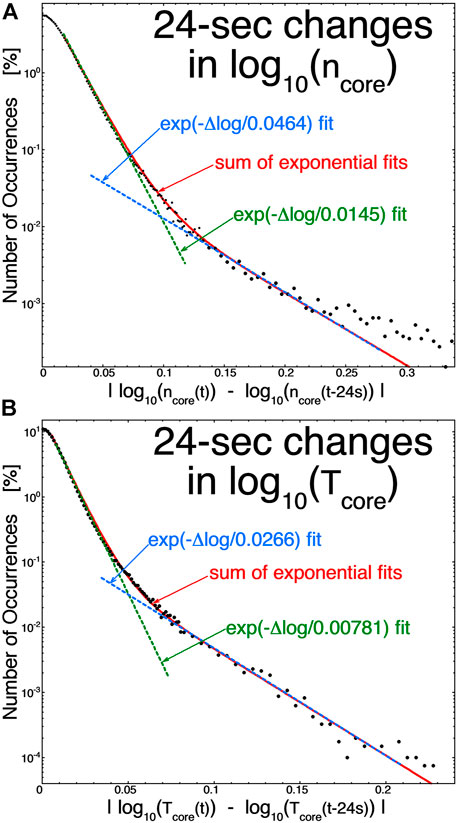
FIGURE 1. The occurrence distribution of the 24-s change in log10(ncore) [panel (A)] and in log10(Tcore) [panel (B)] are binned for 120 days of WIND measurements at 1 AU.
A question that will be addressed is whether or not the boundaries of ncore and of Tcore in the solar wind tend to be co-located with the current sheets of the solar-wind magnetic structure.
To determine whether or not there is a relationship between boundaries of the ncore and Tcore structure and strong current sheets in the solar wind, the 30-s angular change in the magnetic-field direction Δθ is examined when the WIND spacecraft crosses the boundaries. Writing b(t) = B(t)/|B(t)|, the 30-s angular change in the magnetic-field direction at time t is calculated from the magnetic-field vector time series as
In Figure 2 some occurrence distributions of the 30-s change in the magnetic-field direction Δθ are plotted. The black points in Figure 2 plot the distribution of Δθ values for all times during the first 120 days of 2005, with the exclusion of times when the WIND spacecraft was in ejecta plasma. Note the two components to the black-point Δθ distribution, a small-angle component fit by exp(−Δθ/7.67o) (green dashed curve) and a large-angle component fit by exp(−Δθ/25.5o) (purple dashed curve). The solid-red curve is the sum of the two exponential fits [See also Figure 2 of Borovsky (2008) and Figure 6 of Miao et al. (2011) for similar two-component Δθ distributions]. The large-Δθ portion of the distribution has been interpreted as representing crossings of strong current sheets in the solar wind (Burlaga and Ness, 1969; Knetter et al., 2004; Borovsky, 2008) (flux-tube walls between one flux tube and its neighbor) and the small-Δθ portion of the distribution has been taken to represent small magnetic-field fluctuations in the interiors of the flux tubes. The large Δθ component of the black-point distribution is expected to extend down to smaller values of Δθ below the breakpoint in the curve: the red solid curve matching the black points is the sum of the two exponential fits. In the spaghetti of magnetic flux tubes, the angle of the magnetic-field direction in one tube with vs. the neighboring flux tube is a function of the distance along a tube so that sometimes the Δθ value crossing between tubes is large and sometimes the Δθ value is small, even zero. Hence, using the large-Δθ criterion to find flux-tube walls will fail to locate some of the walls (The walls sometimes can be located via other properties, such as jumps in the plasma properties). The mean value of Δθ for the exp (−Δθ/25.5o) is <Δθ > = 25.5o and the mean value of Δθ for the entire black-point distribution (the sum of the two exponential fits) is <Δθ> = 10.2o. The blue points in Figure 2 plot the distribution of 30-s Δθ values during the times when jumps (boundaries) in ncore are seen. Those blue data points are fit with an exponential function exp(−Δθ/25.8o) (dark-blue dashed curve), which is similar to the exp(−Δθ/25.5o) large-Δθ fit of the current-sheet crossings for the black-point distribution in Figure 2. Note that this blue-point distribution extends down into small-Δθ values, which probably represents crossings between flux tubes that are locally nearly aligned at the crossing point. Hence, the Δθ values seen at the times of crossing ncore boundaries in the solar wind (blue points) are consistent with crossings of strong current sheets in the solar wind. The red points in Figure 2 plot the distribution of 30-s Δθ values during the times when jumps (boundaries) in Tcore are seen. Those data points are fit with an exponential function exp(−Δθ/29.6o) (dark-red dashed curve), which is also similar to the exp(−Δθ/25.5o) fit of the current-sheet crossings for the black-point distribution in Figure 2. And note again that this red-point distribution extends down into small Δθ values. Hence, the Δθ values seen at the times of crossing Tcore boundaries in the solar wind are consistent with crossings of strong current sheets in the solar wind (Note, in the collection of ncore and Tcore boundaries, the two boundaries are often co-located).
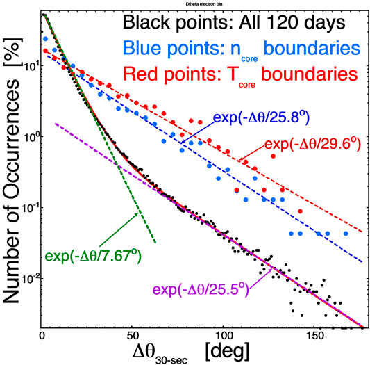
FIGURE 2. Distributions of the 30-s change in the magnetic field direction Δθ are plotted using WIND magnetic-field measurements. The black points are the distribution of all values in the first 120 days of 2005. The blue points are the Δθ values at the times that WIND was crossing boundaries in the core-electron number density and the red points are the Δθ values at the times that WIND was crossing boundaries in the core-electron temperature. The exponential fits are described in the text.
In Figure 3 the superposed epoch average value of the magnetic-field-direction change Δθ is plotted as a function of the time from the identified jumps in the values of ncore. A time shift τshift = 0 in the plot means the 30-s change Δθ in the magnetic-field direction is centered at the times of the ncore jumps, and time shifts away from 0 have the 30-s change Δθ centered at a time τshift away from the jumps in ncore. The individual curves in Figure 3 pertain to the sets of identified ncore boundaries in the different types of solar-wind plasma, as determined using the Xu and Borovsky (2015) plasma-categorization scheme. Excluded in Figure 3 are ncore boundaries found in ejecta plasma; ejecta plasma is often characterized by a smoothly varying magnetic-field direction (Klein and Burlaga, 1982; Cane and Richardson, 2003), a low level of field fluctuations (Lepping et al., 2005; Borovsky et al., 2019), and by a dearth of strong current sheets (Borovsky, 2008; Borovsky, 2012a). Note in Figure 3 that the average value of Δθ is much greater at the time of boundary crossings (τshift = 0) than it is away from the boundaries (τshift ≠ 0): this indicates that the ncore boundaries in the solar wind tend to be co-located with strong current sheets in the solar wind, as was also indicted in Figure 2. The values of Δθ at τshift = 0 in Figure 3 are consistent with the mean value <Δθ> = 25.5o for the exp(−Δθ/25.5o) portion of the black-point distribution in Figure 2. The values of Δθ away from τshift = 0 in Figure 3 are consistent with the <Δθ> = 10.2o found for the total black-point (sheets and not sheets) distribution in Figure 2. Hence, changes in ncore tend to occur when crossing from one magnetic flux tube into another tube. Note in Figure 3 the systematically differing amplitude of Δθ in the different categories of solar-wind plasma (in the different colored curves); these systematic differences in the “wiggle angle” of the magnetic field in the differing plasma types have been explored in prior studies [cf. Figure 11 of Borovsky and Denton (2010) or Figure 8a of Borovsky et al. (2019)].
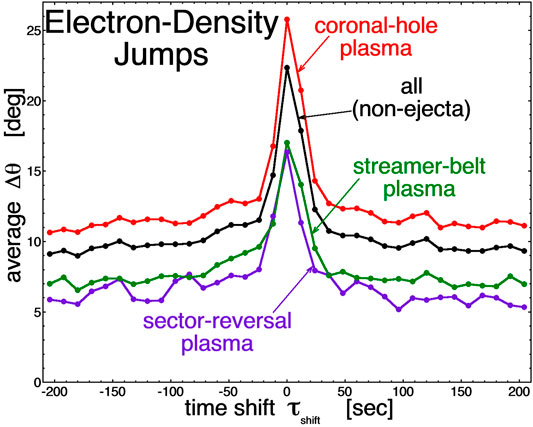
FIGURE 3. The superposed epoch average value of the 30-s change in the magnetic-field direction is plotted as a function of time from the identified core-electron density boundaries in the WIND data set at 1 AU.
Similarly, in Figure 4 the superposed epoch average of Δθ is plotted as a function of the time from the identified jumps in the values of Tcore, with τshift = 0 meaning the 30-s change Δθ in the magnetic-field direction is centered at the times of the Tcore jumps. The individual curves in Figure 4 pertain to the sets of identified Tcore boundaries in the different types of solar-wind plasma. Again, excluded are Tcore boundaries found in ejecta plasma. In Figure 4 the average value of Δθ is much greater at the time of Tcore boundary crossings (τshift = 0) than it is away from the Tcore boundaries (τshift ≠ 0). The values of Δθ at τshift = 0 in Figure 4 are again consistent with the mean value <Δθ> = 25.5o for the exp(−Δθ/25.5o) portion of the black-point distribution in Figure 2, and the values of Δθ away from τshift = 0 in Figure 4 are again consistent with the <Δθ> = 10.2o found for the total black-point (sheets and not sheets) distribution in Figure 2. Figure 4 indicates that the Tcore boundaries in the solar wind tend to be co-located with strong current sheets in the solar wind, as was also indicted in Figure 2. Hence, Tcore changes tend to occur when crossing from one magnetic flux tube into another tube.
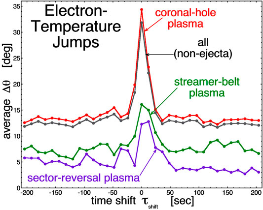
FIGURE 4. The superposed epoch average value of the 30-s change in the magnetic-field direction is plotted as a function of time from the identified core-electron temperature boundaries in the WIND data set at 1 AU. Note that the statistics of the purple sector-reversal-region-plasma curve are poor with only 29 identified temperature-boundary events.
Going back to the two component Δθ distribution of Figure 2, one can ask the question: What fraction of current-sheet crossings do not have Δθ values large enough to be detected out of the noise of the small-Δθ distribution. For the small-Δθ component of the black-point distribution of Figure 2 that is fit by exp (−Δθ/7.67o), 95% of the points in that distribution have Δθ < 23.0o. A Δθ value for an electron boundary that is greater than 23.0o would probably stand out in a time series from the values of the background. Assuming that the exp(−Δθ/25.5o) distribution of current-sheet crossings extends down to Δθ = 0o (as do the red-point and blue-point distributions in Figure 2), then 41% of the points in the exp(−Δθ/25.5o) distribution have Δθ > 23.0o. Hence, about half (41%) of the cold-electron boundaries are expected to be individually identified as current-sheet crossings and about half (59%) are expected to have Δθ values too low to be clearly identified as current-sheet crossings, although they probably are.
In Figure 5 the amplitudes of the identified jumps in ncore (Figure 5A) and the identified jumps in Tcore (Figure 5B) are examined. Here the occurrence distributions of the jump amplitudes are plotted, where the amplitudes are binned with linear bin sizes but plotted logarithmically. The jump amplitude here is measured by the absolute value of the difference between the average of the values of the four data points before the jump and the average of the values of the four data points after the jump. As seen in Figure 5A, typical jump values of ncore are ∼1 cm−3, with values as large as 5 cm−3 being not uncommon. Figure 5B displays the distribution of jump amplitudes for Tcore: typical values are ∼1 eV and values of 5 eV or so are not uncommon.
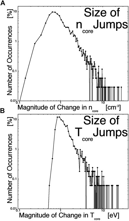
FIGURE 5. The distributions of jump sizes for the identified number-density boundaries [panel (A)] and for the identified temperature boundaries [panel (B)] are plotted. Note that the binning used linear bi sizes (horizontal axis), but the bin values are plotted logarithmically.
Examination of Parker Solar Probe Measurements Near the Sun
A brief, non-statistical examination is made of core electron measurements by the Parker Solar Probe spacecraft during the January-2020 close encounter with the Sun. Figures 6, 7 plot two time series of the temperature Tcore of the core-electron population (blue) along with the 10-s change in the magnetic-field direction Δθ (green). Jumps in the value of Tcore are indicated by vertical dashed line segments: these jumps are identified by visual inspection of the time series and they are not identified with the 8-point numerical algorithm [expression (1)] that was used to identify jumps in the WIND time series at 1 AU. Jumps in the value of Tcore that are associated with strong changes Δθ in the field direction are denoted with red vertical dashed line segments and jumps in the value of Tcore that are not associated with strong changes Δθ in the field direction are denoted with light-blue vertical dashed line segments. Figure 6 plots 48 min of measurements at 0.13 AU on January 29, 2020 and Figure 7 plots 15.6 min of measurements at 0.13 AU on January 30, 2020. In Figure 6 six jumps in Tcore are marked with red vertical segments indicating that they are associated with localized large Δθ values, i.e., these shifts in the Tcore value are associated with crossings of strong current sheets in the solar wind. In Figure 6 six jumps in Tcore are marked with light-blue vertical segments indicating that they are not associated with crossings of current sheets in the solar wind that are strong enough to have Δθ values larger than the background values. (This is also the case for Tcore jumps at 1 AU, as discussed in The WIND Statistical Data Analysis at 1 AU and as shown by the red-point distribution in Figure 2, where the distribution of Δθ values for Tcore jumps extends down to low Δθ values.) Those low-Δθ Tcore jumps could be interpreted as jumps associated with flux tubes that are locally near parallel where the spacecraft crosses from one tube into the next. In Figure 7 all six observed shifts in Tcore are associated with strong current-sheet crossings (red dashed line segments). Note in Figure 7 the magnitude of the Δθ values at the times of the Tcore jumps, often showing a magnetic-field rotation of more than 90o across the current sheets. The examination of the two time series in Figures 6, 7 indicates that, at 0.13 AU, the spatial structure of the core electron temperature Tcore is related to the magnetic-flux-tube structure, as it is at 1 AU.
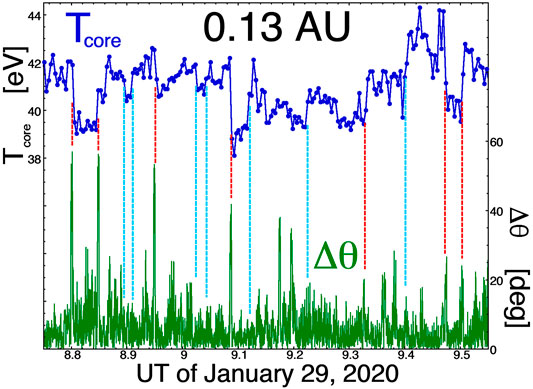
FIGURE 6. For 48 min of time-series measurements by Parker Solar Probe on January 29, 2020 the relationship between jumps in the core-electron temperature (blue curve) and current-sheet crossings as indicated by strong temporal changes in the magnetic-field direction (green curve) are examined.
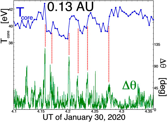
FIGURE 7. For 15.6 min of time-series measurements by Parker Solar Probe on January 30, 2020 the relationship between jumps in the core-electron temperature (blue curve) and current-sheet crossings as indicated by strong temporal changes in the magnetic-field direction (green curve) are examined.
Note that none of the Tcore changes flagged in Figures 6, 7 are associated with magnetic switchbacks (field foldings or field inversions), which at times are prevalent in the Parker Solar Probe data set (Dudok de Wit et al., 2020; Macneil et al., 2020). The closest is the event at 4.203 UT in Figure 7, where the magnetic field makes a transition to a near-radial orientation from a transverse-to-radial orientation.
Typical changes in the value of Tcore in the jumps marked in Figures 6, 7 are 2–3 eV.
Summary and Discussion
A statistical analysis of 120 days of solar-wind measurements at 1 AU show that the density structure and temperature structure of the core electrons of the solar wind are both related to the magnetic-flux-tube structure of the solar wind; in this structure the number density ncore and temperature Tcore of the core-electron population tend to jump in value from flux tube to flux tube. An examination of Tcore measurements at 0.13 AU shows the same features related to the magnetic structure, with Tcore jumps associated with current-sheet crossings.
The relationship between the electron number density ncore and the magnetic flux tubes is no surprise in light of quasi-neutrality considerations, since it is known that the proton number density structure of the solar wind reflects the magnetic structure (Borovsky, 2012b; Borovsky, 2020b). The variations in Tcore that are related to the magnetic-flux-tube structure are more interesting. If a local value of Tcore represents a measurement of the local electrical potential ϕ, then Tcore varying from tube to tube means ϕ varies from tube to tube. If ϕ(r) is (as in an exosphere model) determined by the evolution of the solar-wind ions and electrons away from the Sun, then variations of ϕ from tube to tube might mean that exosphere models apply tube by tube, i.e., that the solar-wind evolution is to some degree independent from tube to tube. There is no reason to argue that the differing flux tubes should not act independently. At 1 AU it is seen that the intensity of the electron stralh can vary from flux tube to flux tube (Borovsky, 2021): this strahl variation is an indication that different flux tubes at 1 AU are connected to different features in the corona (Gosling et al., 2004a,b; Borovsky, 2021). The differences in connection to the corona could result in independent exospheric scenarios in the different flux tubes.
If the solar-wind plasma is an admixture of open flux tubes plus other magnetic structures (e.g., Figure 24C of Khabarova et al., 2021) then the exosphere-model picture is more complicated. Further investigation of field and core-electron measurements at 1 AU, guided with measurements of the strahl intensity to judge magnetic connectivity to the Sun (Borovsky, 2021), is called for. In any closed-magnetic structure, the interpretation of Tcore as an indication of the local electrical potential ϕ (e.g., Feldman et al., 1975; Boldyrev et al., 2020; Moncuquet et al., 2020) might no longer be possible.
At both 1 and 0.13 AU, the fractional variation of Tcore in a typical jump is about 10% of the value of Tcore, although occasional much-larger jumps (several tens of percent) can be found. This indicates a variation of the interplanetary potential of about 10% from tube to tube, although not every tube-wall crossing shows a jump in Tcore.
At 1 AU typical Tcore changes across flux-tube walls are ∼1 eV, although larger potentials can be found. This represents a change in electrical potential of ∼1 V across the boundary between adjacent flux tubes. If at 1 AU a current sheet (flux-tube wall) is 1,000-km thick (e.g., Siscoe et al., 1968; Vasquez et al., 2007) and the potential change is 1 V, then the electric field of this potential change is E = 1 × 10⁻⁶ V/m. For a magnetic field strength of 5 nT, this corresponds to an E × B drift speed of 0.2 km/s [Note that if the potential is a few times the core-electron temperature (cf. Maksimovic et al., 1997), then these electric-field values and drift speeds are a few times larger].
In future, a statistical analysis of the changes in Tcore in the Parker Solar Probe data is needed accounting for the types of plasma being observed and the rapid longitudinal motion of the spacecraft. In particular this will be interesting when future closer passes to the Sun have occurred and the variations of the interplanetary electric potential can be examined where the potentials are anticipated to be greater in magnitude nearer to the Sun.
Data Availability Statement
Publicly available datasets were analyzed in this study. This data can be found here: https://cdaweb.gsfc.nasa.gov/index.html/.
Author Contributions
JB initiated this project, performed the data analysis, and wrote the initial draft of the manuscript. JH and PW prepared the Solar Probe Data and contributed to the final version of the manuscript.
Funding
This work was supported by the NSF SHINE program via grant no AGS-1723416, by the NASA Heliophysics Guest Investigator Program via award NNX17AB71G, by the NSF GEM Program via grant no AGS-2027569, and by the NASA Heliophysics LWS program via award NNX16AB75G. JH and PW were supported by the PSP SWEAP contract NNN06AA01C.
Conflict of Interest
The authors declare that the research was conducted in the absence of any commercial or financial relationships that could be construed as a potential conflict of interest.
Acknowledgments
The authors thank Stas Boldyrev and Vadim Roytershteynure for helpful conversations.
References
Adhikari, L., Khabarova, O., Zank, G. P., and Zhao, L.-L. (2019). The Role of Magnetic Reconnection-Associated Processes in Local Particle Acceleration in the Solar Wind. ApJ 873, 72. doi:10.3847/1538-4357/ab05c6
Bale, S. D., Goetz, K., Harvey, P. R., Turin, P., Bonnell, J. W., de Wit, T. D., et al. (2016). The FIELDS Instrument Suite for Solar Probe Plus: Measuring the Coronal Plasma and Magnetic Field, Plasma Waves and Turbulence, and Radio Signatures of Solar Transients. Space Sci. Rev. 204, 49–82. doi:10.1007/s11214-016-0244-5
Bartley, W. C., Bukata, R. P., McCracken, K. G., and Rao, U. R. (1966). Anisotropic Cosmic Radiation Fluxes of Solar Origin. J. Geophys. Res. 71, 3297–3304. doi:10.1029/jz071i013p03297
Birch, M. J., and Hargreaves, J. K. (2020a). Quasi-periodic Ripples in High-Latitude Electron Content, the Geomagnetic Field, and the Solar Wind. Nat. Scienific Rep 10, 1313. doi:10.1038/s41598-019-57201-4
Birch, M. J., and Hargreaves, J. K. (2020b). Quasi-periodic Ripples in the Heliosphere from 1 to 40 AU. Adv. Space Res. 67, 678.
Boldyrev, S., Forest, C., and Egedal, J. (2020). Electron Temperature of the Solar Wind. Proc. Natl. Acad. Sci. USA 117, 9232–9240. doi:10.1073/pnas.1917905117
Borovsky, J. E., and Denton, M. H. (2010). Solar Wind Turbulence and Shear: A Superposed-Epoch Analysis of Corotating Interaction Regions at 1 AU. J. Geophys. Res. 115, A10101. doi:10.1029/2009ja014966
Borovsky, J. E., and Denton, M. H. (2016). The Trailing Edges of High-Speed Streams at 1 AU. J. Geophys. Res. Space Phys. 121, 6107–6140. doi:10.1002/2016ja022863
Borovsky, J. E., and Steinberg, J. T. (2014). No Evidence for the Localized Heating of Solar Wind Protons at Intense Velocity Shear Zones. J. Geophys. Res. Space Phys. 119, 1455–1462. doi:10.1002/2013ja019746
Borovsky, J. E., Denton, M. H., and Smith, C. W. (2019). Some Properties of the Solar-Wind Turbulence at 1 AU Statistically Examined in the Different Types of Solar-Wind Plasma. J. Geophys. Res. 124, 2406. doi:10.1029/2019JA026580
Borovsky, J. E. (2006). The Eddy Viscosity and Flow Properties of the Solar Wind: CIRs, CME Sheaths, and Solar-Wind/magnetosphere Coupling. Phys. Plasmas 13, 056505. doi:10.1063/1.2200308
Borovsky, J. E. (2008). Flux Tube Texture of the Solar Wind: Strands of the Magnetic Carpet at 1 AU?. J. Geophys. Res. 113, A08110. doi:10.1029/2007ja012684
Borovsky, J. E. (2010). On the Variations of the Solar Wind Magnetic Field about the Parker Spiral Direction. J. Geophys. Res. 115, A09101. doi:10.1029/2009ja015040
Borovsky, J. E. (2012a). The Velocity and Magnetic Field Fluctuations of the Solar Wind at 1 AU: Statistical Analysis of Fourier Spectra and Correlations with Plasma Properties. J. Geophys. Res. 117, A05104. doi:10.1029/2011ja017499
Borovsky, J. E. (2012b). Looking for Evidence of Mixing in the Solar Wind from 0.31 to 0.98 AU. J. Geophys. Res. 117, A06107. doi:10.1029/2012ja017525
Borovsky, J. E. (2020a). The Magnetic Structure of the Solar Wind: Ionic Composition and the Electron Strahl. Geophys. Res. Lett. 47, e2019GL084586. doi:10.1029/2019gl084586
Borovsky, J. E. (2020b). Plasma and Magnetic-Field Structure of the Solar Wind at Inertial-Range Scale Sizes Discerned from Statistical Examinations of the Time-Series Measurements. Front. Astron. Space Sci. 7, 20. doi:10.3389/fspas.2020.00020
Borovsky, J. E. (2020c). On the Motion of the Heliospheric Magnetic Structure through the Solar Wind Plasma. J. Geophys. Res. 125, e2019JA027377. doi:10.1029/2019ja027377
Borovsky, J. E. (2020d). Compression of the Heliospheric Magnetic Structure by Interplanetary Shocks: Is the Structure at 1 AU a Manifestation of Solar-Wind Turbulence or Is it Fossil Structure from the Sun?. Front. Astron. Space Sci. 7, 582546. doi:10.3389/fspas.2020.582564
Borovsky, J. E. (2021). Exploring the Properties of the Electron Strahl at 1 AU as an Indicator of the Quality of the Magnetic Connection between the Earth and the Sun. Front. Astron. Space Sci. 8, 646443. doi:10.3389/fspas.2021.646443
Bruno, R., Carbone, V., Veltri, P., Pietropaolo, E., and Bavassano, B. (2001). Identifying Intermittency Events in the Solar Wind. Planet. Space Sci. 49, 1201–1210. doi:10.1016/s0032-0633(01)00061-7
Burkholder, B. L., Otto, A., Delamere, P. A., and Borovsky, J. E. (2019). Magnetic Connectivity in the corona as a Source of Structure in the Solar Wind. J. Geophys. Res. Space Phys. 124, 32–49. doi:10.1029/2018ja026132
Burlaga, L. F., and Ness, N. F. (1969). Tangential Discontinuities in the Solar Wind. Sol. Phys. 9, 467–477. doi:10.1007/bf02391672
Burlaga, L. F. (1969). Directional Discontinuities in the Interplanetary Magnetic Field. Sol. Phys. 7, 54–71. doi:10.1007/bf00148406
Cane, H. V., and Richardson, I. V. (2003). Interplanetary Coronal Mass Ejections in the Near-Earth Solar Wind during 1996-2002. J. Geophys. Res. 108, 1156. doi:10.1029/2002ja009817
Close, R. M., Parnell, C. E., MacKay, D. H., and Priest, E. R. (2003). Statistical Flux Tube Properties of 3D Magnetic Carpet fields. Solar Phys. 212, 251–275. doi:10.1023/a:1022961913168
Close, R. M., Parnell, C. E., and Priest, E. R. (2005). Separators in 3D Quiet-Sun Magnetic fields. Solar Phys. 225, 21. doi:10.1023/A:1022961913168
Colburn, D. S., and Sonett, C. P. (1966). Discontinuities in the Solar Wind. Space Sci. Rev. 5, 439. doi:10.1007/bf00240575
DeForest, C. E., Howard, R. A., Velli, M., Viall, N., and Vourlidas, A. (2018). The Highly Structured Outer Solar corona. ApJ 862, 18. doi:10.3847/1538-4357/aac8e3
Di Matteo, S., Viall, N. M., Kepko, L., Wallace, S., Arge, C. N., and MacNeice, P. (2019). Helios Observations of Quasiperiodic Density Structures in the Slow Solar Wind at 0.3, 0.4, and 0.6 AU. J. Geophys. Res. Space Phys. 124, 837–860. doi:10.1029/2018ja026182
Dmitruk, P., Matthaeus, W. H., and Seenu, N. (2004). Test Particle Energization by Current Sheets and Nonuniform fields in Magnetohydrodynamic Turbulence. ApJ 617, 667–679. doi:10.1086/425301
Dobrowolny, M., Mangeney, A., and Veltri, P. (1980). Fully Developed Anisotropic Hydromagnetic Turbulence in Interplanetary Space. Phys. Rev. Lett. 45, 144–147. doi:10.1103/physrevlett.45.144
Doss, C. E., Komar, C. M., Cassak, P. A., Wilder, F. D., Eriksson, S., and Drake, J. F. (2015). Asymmetric Magnetic Reconnection with a Flow Shear and Applications to the Magnetopause. J. Geophys. Res. Space Phys. 120, 7748–7763. doi:10.1002/2015ja021489
Dudok de Wit, T., Krasnoselskikh, V. V., Bale, S. D., Bonnell, J. W., Bowen, T. A., Chen, C. H. K., et al. (2020). Switchbacks in the Near-Sun Magnetic Field: Long Memory and Impact on the Turbulence cascade. ApJS 246, 39. doi:10.3847/1538-4365/ab5853
Eselevich, V. G. (2019). Diamagnetic Structures as a Basis of Quasi-Stationary Slow Solar Wind. Solar-terr. Phys. 5 (3), 29.
Feldman, W. C., Asbridge, J. R., Bame, S. J., Montgomery, M. D., and Gary, S. P. (1975). Solar Wind Electrons. J. Geophys. Res. 80, 4181–4196. doi:10.1029/ja080i031p04181
Feldman, W. C., Asbridge, J. R., Bame, S. J., Gosling, J. T., and Lemons, D. S. (1978). Characteristic Electron Variations across Simple High-Speed Solar Wind Streams. J. Geophys. Res. 83, 5285. doi:10.1029/ja083ia11p05285
Gosling, J. T., de Koning, C. A., Skoug, R. M., Steinberg, J. T., and McComas, D. J. (2004a). Dispersionless Modulations in Low-Energy Solar Electron Bursts and Discontinuous Changes in the Solar Wind Electron Strahl. J. Geophys. Res. 109, A05102. doi:10.1029/2003ja010338
Gosling, J. T., Skoug, R. M., McComas, D. J., and Mazur, J. E. (2004b). Correlated Dispersionless Structure in Suprathermal Electrons and Solar Energetic Ions in the Solar Wind. ApJ 614, 412–419. doi:10.1086/423368
Gosling, J. T., Skoug, R. M., McComas, D. J., and Smith, C. W. (2005). Direct Evidence for Magnetic Reconnection in the Solar Wind Near 1 AU. J. Geophys. Res. 110, A01107. doi:10.1029/2004ja010809
Gosling, J. T. (2012). Magnetic Reconnection in the Solar Wind. Space Sci. Rev. 172, 187–200. doi:10.1007/s11214-011-9747-2
Greco, A., Chuychai, P., Matthaeus, W. H., Servidio, S., and Dmitruk, P. (2008). Intermittent MHD Structures and Classical Discontinuities. Geophys. Res. Lett. 35, L19111. doi:10.1029/2008gl035454
Greco, A., Matthaeus, W. H., Servidio, S., Dmitruk, P., Wan, M., Oughton, S., et al. (2010). Statistical Propertie of Solar Wind Discontinuities, Intermittent Turbulence, and Rapid Emergence of Non-gaussian Distribution. AIP Conf. Proc. 1216, 202. doi:10.1063/1.3395836
Greco, A., Perri, S., Servidio, S., Yordanova, E., and Veltri, P. (2016). The Complex Structure of Magnetic Field Discontinuities in the Turbulent Solar Wind. ApJ 823, L39. doi:10.3847/2041-8205/823/2/l39
Halekas, J. S., Whittlesey, P., Larson, D. E., McGinnis, D., Maksimovic, M., Berthomier, M., et al. (2020). Electrons in the Young Solar Wind: First Results from the Parker Solar Probe. ApJS 246, 22. doi:10.3847/1538-4365/ab4cec
Hannum, D., Bateman, G., Kinsey, J., Kritz, A. H., Onjun, T., and Pankin, A. (2001). Comparison of High-Mode Predictive Simulations Using Mixed Bohm/gyro-Bohm and Multi-Mode (MMM95) Transport Models. Phys. Plasmas 8, 964–974. doi:10.1063/1.1338534
Hesse, M., Birn, J., and Kuznetsova, M. (2001). Collisionless Magnetic Reconnection: Electron Processes and Transport Modeling. J. Geophys. Res. 106, 3721–3735. doi:10.1029/1999ja001002
Huang, C., Yan, Y., Li, G., Deng, Y., and Tan, B. (2014). Tracking Back the Solar Wind to its Photospheric Footpoints from Wind Observations - A Statistical Study. Sol. Phys. 289, 3109–3119. doi:10.1007/s11207-014-0508-8
Kasper, J. C., Abiad, R., Austin, G., Balat-Pichelin, M., Bale, S. D., Belcher, J. W., et al. (2016). Solar Wind Electrons Alphas and Protons (SWEAP) Investigation: Design of the Solar Wind and Coronal Plasma Instrument Suite for Solar Probe Plus. Space Sci. Rev. 204, 131–186. doi:10.1007/s11214-015-0206-3
Kepko, L., and Spence, H. E. (2003). Observations of Discrete, Global Magnetospheric Oscillations Directly Driven by Solar Wind Density Variations. J. Geophys. Res. 108, 1257. doi:10.1029/2002ja009676
Kepko, L., and Viall, N. M. (2019). The Source, Significance, and Magnetospheric Impact of Periodic Density Structures within Stream Interaction Regions. J. Geophys. Res. 124, 2019JA026962. doi:10.1029/2019ja026962
Kepko, L., Viall, N. M., Antiochos, S. K., Lepri, S. T., Kasper, J. C., and Weberg, M. (2016). Implications of L1 Observations for Slow Solar Wind Formation by Solar Reconnection. Geophys. Res. Lett. 43, 4089–4097. doi:10.1002/2016gl068607
Khabarova, O., Zharkova, V., Xia, Q., and Malandraki, O. E. (2020). Counterstreaming Strahls and Heat Flux Dropouts as Possible Signatures of Local Particle Acceleration in the Solar Wind. ApJ 894, L12. doi:10.3847/2041-8213/ab8cb8
Khabarova, O., Malandraki, O., malova, H., Kislov, R., Greco, A., Bruno, R., et al. (2021). Current Sheets, Plasmoids and Flux Ropes in the Heliosphere. Space Sci. Rev. 217, 38. doi:10.1007/s11214-021-00814-x
Khaborova, O., Zank, G., Li, G., Le Roux, J. A., Webb, G. M., Dosch, A., et al. (2015). Small-scale Magnetic Islands in the Solar Wind and Their Role in Particle Acceleration. I. Dynamics of Magnetic Islands Near the Heliospheric Current Sheet. Astrophys. J. 808, 181. doi:10.1088/0004-637X/808/2/181
Khaborova, O., Zank, G., Li, G., MalandrakiLe Roux, O. E. J. A., and Webb, G. M. (2016). Small-scale Magnetic Islands in the Solar Wind and Their Role in Particle Acceleration. II. Particle Energization inside Magnetically Confined Cavities. Astrophys. J. 827, 122. doi:10.3847/0004-637X/827/2/122
Klein, L. W., and Burlaga, L. F. (1982). Interplanetary Magnetic Clouds at 1 AU. J. Geophys. Res. 87, 613. doi:10.1029/ja087ia02p00613
Knetter, T., Neubauer, F. M., Horbury, T., and Balogh, A. (2003). Discontinuity Observations with Cluster. Adv. Space Res. 32 (4), 543–548. doi:10.1016/s0273-1177(03)00335-1
Knetter, T., Neubauer, F. M., Horbury, T., and Balogh, A. (2004). Four-point Discontinuity Observations Using Cluster Magnetic Field Data: A Statistical Survey. J. Geophys. Res. 109, A06102. doi:10.1029/2003ja010099
Lacombe, C., Salem, C., Mangeney, A., Hubert, D., Perche, C., Bougeret, J.-L., et al. (2002). Evidence for the Interplanetary Electric Potential? WIND Observations of Electrostatic Fluctuations. Ann. Geophys. 20, 609–618. doi:10.5194/angeo-20-609-2002
Lemaire, J., and Scherer, M. (1971). Simple Model for an Ion-Exosphere in an Open Magnetic Field. Phys. Fluids 14, 1683. doi:10.1063/1.1693664
Lemaire, J. (2010). Half a century of Kinetic Solar Wind Models. AIP Conf. Proc. 1216, 8. doi:10.1063/1.3395971
Lemons, D. S., and Feldman, W. C. (1983). Collisional Modification to the Exospheric Theory of Solar Wind Halo Electron Pitch Angle Distributions. J. Geophys. Res. 88, 6881. doi:10.1029/ja088ia09p06881
Lepping, R. P., Acũna, M. H., Burlaga, L. F., Farrell, W. M., Slavin, J. A., Schatten, K. H., et al. (1995). The WIND Magnetic Field Investigation. Space Sci. Rev. 71, 207–229. doi:10.1007/bf00751330
Lepping, R. P., Wu, C.-C., and Berdichevsky, D. B. (2005). Automatic Identification of Magnetic Clouds and Cloud-like Regions at 1 AU: Occurrence Rate and Other Properties. Ann. Geophys. 23, 2687–2704. doi:10.5194/angeo-23-2687-2005
Li, G. (2008). Identifying Current-sheet-like Structures in the Solar Wind. ApJ 672, L65–L68. doi:10.1086/525847
Lie-Svendsen, Ø., and Leer, E. (2000). The Electron Velocity Distribution in the High-Speed Solar Wind: Modeling the Effects of Protons. J. Geophys. Res. 105, 35–46. doi:10.1029/1999ja900438
Macneil, A. R., Owens, M. J., Wicks, R. T., Lockwood, M., Bentley, S. N., and Lang, M. (2020). The Evolution of Inverted Magnetic fields through the Inner Heliosphere. Mon. Not. R. Astron. Soc. 494, 3655. doi:10.1093/mnras/staa951
Maksimovic, M., Pierrard, V., and Lemaire, J. F. (1997). A Kinetic Model of the Solar Wind with Kappa Distribution Functions in the corona. Astron. Astrophys. 324, 725.
Maksimovic, M., Zouganelis, I., Chaufray, J.-Y., Issautier, K., Scime, E. E., Littleton, J. E., et al. (2005). Radial Evolution of the Electron Distribution Functions in the Fast Solar Wind between 0.3 and 1.5 AU. J. Geophys. Res. 110, A09104. doi:10.1029/2005ja011119
Malandraki, O., Khabarova, O., Bruno, R., Zank, G. P., Li, G., Jackson, B., et al. (2019). Current Sheets, Magnetic Islands, and Associated Particle Acceleration in the Solar Wind as Observed by Ulysses Near the Ecliptic Plane. ApJ 881, 116. doi:10.3847/1538-4357/ab289a
Malara, F., Primavera, L., and Veltri, P. (1996). Gompressive Fluctuations Generated by Time Evolution of Alfvénic Perturbations in the Solar Wind Current Sheet. J. Geophys. Res. 101, 21597–21617. doi:10.1029/96ja01637
Mariani, F., Bavassano, B., Villante, U., and Ness, N. F. (1973). Variations of the Occurrence Rate of Discontinuities in the Interplanetary Magnetic Field. J. Geophys. Res. 78, 8011–8022. doi:10.1029/ja078i034p08011
Marsch, E. (2006). Kinetic Physics of the Solar corona and Solar Wind. Living Rev. Solar Phys. 3, 1. doi:10.12942/lrsp-2006-1
Matthaeus, W. H., Montgomery, D. C., Wan, M., and Servidio, S. (2012). A Review of Relaxation and Structure in Some Turbulent Plasmas: Magnetohydrodynamic and Related Models. J. Turb. 37, 1.
McComas, D. J., Bame, S. J., Feldman, W. C., Gosling, J. T., and Phillips, J. L. (1992). Solar Wind Halo Electrons from 1-4 AU. Geophys. Res. Lett. 19, 1291–1294. doi:10.1029/92gl00631
McCracken, K. G., and Ness, N. F. (1966). The Collimation of Cosmic Rays by the Interplanetary Magnetic Field. J. Geophys. Res. 71, 3315–3318. doi:10.1029/jz071i013p03315
Meyer-Vernet, N., and Issautier, K. (1998). Electron Temperature in the Solar Wind: Generic Radial Variation from Kinetic Collisionless Models. J. Geophys. Res. 103, 29705–29717. doi:10.1029/98ja02853
Meyer-Vernet, N., Mangeney, A., Maksimovic, M., Pantellini, F., and Issaurtier, K. (2003). Some Basic Aspects of Solar Wind Acceleration. AIP Conf. Proc. 679, 263. doi:10.1063/1.1618591
Miao, B., Peng, B., and Li, G. (2011). Current Sheets from Ulysses Observation. Ann. Geophys. 29, 237–249. doi:10.5194/angeo-29-237-2011
Michel, F. C. (1967). Model of Solar Wind Structure. J. Geophys. Res. 72, 1917–1932. doi:10.1029/jz072i007p01917
Moncuquet, M., Meyer-Vernet, N., Issautier, K., Pulupa, M., Bonnell, J. W., Bale, S. D., et al. (2020). First In Situ Measurements of Electron Density and Temperature from Quasi-thermal Noise Spectroscopy with Parker Solar Probe/FIELDS. ApJS 246, 44. doi:10.3847/1538-4365/ab5a84
Neugebauer, M., and Giacalone, J. (2010). Progress in the Study of Interplanetary Discontinuities. AIP Conf. Proc. 1216, 194. doi:10.1063/1.3395834
Neugebauer, M., and Giacalone, J. (2015). Energetic Particles, Tangential Discontinuities, and Solar Flux Tubes. J. Geophys. Res. Space Phys. 120, 8281–8287. doi:10.1002/2015ja021632
Ogilvie, K. W., Chornay, D. J., Fritzenreiter, R. J., Hunsaker, F., Keller, J., Lobell, J., et al. (1995). SWE, a Comprehensive Plasma Instrument for the WIND Spacecraft. Space Sci. Rev. 71, 55–77. doi:10.1007/bf00751326
Owens, M. J., Wicks, R. T., and Horbury, T. S. (2011). Magnetic Discontinuities in the Near-Earth Solar Wind: Evidence of In-Transit Turbulence or Remnants of Coronal Structure?. Sol. Phys. 269, 411–420. doi:10.1007/s11207-010-9695-0
Pecora, F., Greco, A., Hu, Q., Servidio, S., Chasapis, A. G., and Matthaeus, W. H. (2019). Single-spacecraft Identification of Flux Tubes and Current Sheets in the Solar Wind. ApJ 881, L11. doi:10.3847/2041-8213/ab32d9
Perkins, F. W., Barnes, C. W., Johnson, D. W., Scott, S. D., Zarnstorff, M. C., Bell, M. G., et al. (1993). Nondimensional Transport Scaling in the Tokamak Fusion Test Reactor: Is Tokamak Transport Bohm or gyro‐Bohm?. Phys. Fluids B: Plasma Phys. 5, 477–498. doi:10.1063/1.860534
Phan, T. D., Gosling, J. T., Davis, M. S., Skoug, R. M., Øieroset, M., Lin, R. P., et al. (2006). A Magnetic Reconnection X-Line Extending More Than 390 Earth Radii in the Solar Wind. Nature 439, 175–178. doi:10.1038/nature04393
Pilipp, W. G., Miggenrieder, H., Mühläuser, K.-H., Rosenbauer, H., and Schwenn, R. (1990). Large-scale Variations of thermal Electron Parameters in the Solar Wind between 0.3 and 1 AU. J. Geophys. Res. 95, 6305. doi:10.1029/ja095ia05p06305
Pritchett, P. L. (2005). The “Newton Challenge”: Kinetic Aspects of Forced Magnetic Reconnection. J. Geophys. Res. 110, A10213. doi:10.1029/2005ja011228
Riazantseva, M. O., Budaev, V., Rakhmanova, L., Zastenker, G., Yermolaev, Y., Lodkina, I., et al. (2017). Variety of Shapes of Solar Wind Ion Flux Spectra: Spektr-R Measurements. J. Plasma Phys. 83, 705830401. doi:10.1017/s0022377817000502
Roth, M., De Keyser, J., and Kuznetsova, M. M. (1996). Vlasov Theory of the Equilibrium Structure of Tangential Discontinuities in Space Plasmas. Space Sci. Rev. 76, 251–317. doi:10.1007/bf00197842
Salem, C., Lacombe, C., Mangeney, A., Kellogg, P. J., and Bougeret, J.-L. (2003). Weak Double Layers in the Solar Wind and Their Relation to the Interplanetary Electric Field. AIP Conf. Proc. 679, 513. doi:10.1063/1.1618647
Scudder, J. D. (2019). Steady Electron Runaway Model SERM: Astrophysical Alternative for the Maxwellian assumption. ApJ 885, 138. doi:10.3847/1538-4357/ab4882
Servidio, S., Gurgiolo, C., Carbone, V., and Goldstein, M. L. (2014). Relaxation Processes in Solar Wind Turbulence. ApJ 789, L44. doi:10.1088/2041-8205/789/2/l44
Sheeley, N. R., and Rouillard, A. P. (2010). Tracking Streamer Blobs into the Heliosphere. ApJ 715, 300–309. doi:10.1088/0004-637x/715/1/300
Siscoe, G. L., Davis, L., Coleman, P. J., Smith, E. J., and Jones, D. E. (1968). Power Spectra and Discontinuities of the Interplanetary Magnetic Field: Mariner 4. J. Geophys. Res. 73, 61–82. doi:10.1029/ja073i001p00061
Telloni, D., Perri, S., Carbone, V., and Bruno, R. (2016). Selective Decay and Dynamic Alignment in the MHD Turbulence: the Role of the Rugged Invariants. AIP Conf. Proc. 1720, 040015. doi:10.1063/1.4943826
Trenchi, L., Bruno, R., Telloni, D., D'amicis, R., Marcucci, M. F., Zurbuchen, T. H., et al. (2013a). Solar Energetic Particle Modulations Associated with Coherent Magnetic Structures. ApJ 770, 11. doi:10.1088/0004-637x/770/1/11
Trenchi, L., Bruno, R., D'Amicis, R., Marcucci, M. F., and Telloni, D. (2013b). Observations of IMF Coherent Structures and Their Relationship to SEP Dropout Events. Ann. Geophys. 31, 1333–1341. doi:10.5194/angeo-31-1333-2013
Tu, C. Y., Wang, X., He, J., Marsch, E., and Wang, L. (2016). Two Cases of Convecting Structure in the Slow Solar Wind Turbulence. AIP Conf. Proc. 1720, 040017. doi:10.1063/1.4943828
Vasquez, B. J., and Hollweg, J. V. (1999). Formation of Pressure-Balanced Structures and Fast Waves from Nonlinear Alfvén Waves. J. Geophys. Res. 104, 4681–4696. doi:10.1029/1998ja900090
Vasquez, B. J., Abramenko, V. I., Haggerty, D. K., and Smith, C. W. (2007). Numerous Small Magnetic Field Discontinuities of Bartels Rotation 2286 and the Potential Role of Alfvénic Turbulence. J. Geophys. Res. 112, A11102. doi:10.1029/2007ja012504
Viall, N. M., and Borovsky, J. E. (2020). Nine Outstanding Questions of Solar Wind Physics. J. Geophys. Res. 125, e2018JA026005. doi:10.1029/2018ja026005
Viall, N. M., and Vourlidas, A. (2015). Periodic Density Structures and the Origin of the Slow Solar Wind. ApJ 807, 176. doi:10.1088/0004-637x/807/2/176
Viall, N. M., Kepko, L., and Spence, H. E. (2009). Relative Occurrence Rates and Connection of Discrete Frequency Oscillations in the Solar Wind Density and Dayside Magnetosphere. J. Geophys. Res. 114, A01201. doi:10.1029/2008ja013334
Viall, N. M., Spence, H. E., Vourlidas, A., and Howard, R. (2010). Examining Periodic Solar-Wind Density Structures Observed in the SECCHI Heliospheric Imagers. Sol. Phys. 267, 175–202. doi:10.1007/s11207-010-9633-1
Wang, Y.-M., Sheeley, N. R., Howard, R. A., Rich, N. B., and Lamy, P. L. (1999). Streamer Disconnection Events Observed with the LASCO Coronagraph. Geophys. Res. Lett. 26, 1349–1352. doi:10.1029/1999gl900177
Whittlesey, P. L., Larson, D. E., Kasper, J. C., Halekas, J., Abatcha, M., Abiad, R., et al. (2020). The Solar Probe ANalyzers-Electrons on the Parker Solar Probe. ApJS 246, 74. doi:10.3847/1538-4365/ab7370
Keywords: solar wind, heliosphere, interplanetary potential, corona, magnetic structure
Citation: Borovsky JE, Halekas JS and Whittlesey PL (2021) The Electron Structure of the Solar Wind. Front. Astron. Space Sci. 8:690005. doi: 10.3389/fspas.2021.690005
Received: 01 April 2021; Accepted: 24 May 2021;
Published: 08 June 2021.
Edited by:
Daniele Telloni, National Institute of Astrophysics (INAF), ItalyReviewed by:
Tommaso Alberti, Institute for Space Astrophysics and Planetology (INAF), ItalyOlga Malandraki, National Observatory of Athens, Greece
Copyright © 2021 Borovsky, Halekas and Whittlesey. This is an open-access article distributed under the terms of the Creative Commons Attribution License (CC BY). The use, distribution or reproduction in other forums is permitted, provided the original author(s) and the copyright owner(s) are credited and that the original publication in this journal is cited, in accordance with accepted academic practice. No use, distribution or reproduction is permitted which does not comply with these terms.
*Correspondence: Joseph E. Borovsky, amJvcm92c2t5QHNwYWNlc2NpZW5jZS5vcmc=