Statistical analysis of overlapping double ion energy dispersion events in the northern cusp

This article presents a statistical analysis of overlapping double ion-energy dispersion events in the northern cusp (“double dispersion”). Double dispersion in either cusp is a phenomenon associated with multiple reconnections occurring on the dayside magnetosphere as a result of its constant interaction with the variable solar wind. Using observations from a low Earth orbiting (LEO) Defense Meteorological Satellite Program (DMSP) satellite, we analyze 138 dayside events selected by the automatic algorithm extended from our previous work. We conducted a correlation study between the number of detected double dispersion events and 1) the month of the year to analyze the seasonal response of the cusp, and 2) solar wind interplanetary magnetic field (IMF) components and clock/cone angles to investigate its relationship with magnetic reconnection. We found that dispersion events occur more frequently during the northern summer months (i.e., when the dipole is tilted Sunward) and when the B_y component of IMF is positive. In addition, we provide a machine-readable list of the events and the code used to automatically detect the events.

1 Introduction

Magnetic reconnection is an important fundamental process that occurs in the magnetosphere and is responsible for phenomena on multiple scales, including geomagnetic storms, aurora, and radiation belt enhancement. However, detailed knowledge of precisely when, where, and how it occurs has challenged the research community since the dawn of the space age. The largest scale reconnection occurs between solar wind and the Earth’s magnetic field. This interaction is theorized to occur on the dayside magnetopause from where energetic particles precipitate to the northern and southern cusps (Reiff et al., 1977; Burch et al., 1982).

The most direct method of studying magnetopause reconnection in the magnetosphere is accomplished by flying appropriately instrumented spacecraft through the daysidemagnetopause, as performed many times during the Magnetospheric Multiscale (MMS) Mission era (Burch et al., 2016a; Burch et al., 2016b) and with the previous missions such as Cluster (Escoubet et al., 2001; Retinò et al., 2006; Pitout and Bogdanova, 2021), THEMIS (Sibeck and Angelopoulos, 2008), Geotail (Nishida, 1994), and ISEE (Paschmann et al., 1979; Sonnerup et al., 1981). The catalog of events collected through this approach is notable but limited, owing to the long orbital period (with scales of days to a week) required to visit the magnetopause. Furthermore, there is a low probability that reconnection occurs within the proximity to a spacecraft rapidly crossing the magnetopause. Furthermore, most missions designed to sample the dayside magnetopause are highly elliptical and undergo orbital precession during the year, leading to seasons when the spacecraft does not sample the dayside magnetosphere at all. Major missions subject to this precession effect include MMS (Fuselier et al., 2016) and Time History of Events and Macroscale Interactions during Substorms (THEMIS) (Frey et al., 2008). To begin answering questions regarding when, where, and how often different types of magnetopause reconnection scenarios occur through a statistical analysis, it is desirable to use a method with more frequent observation opportunities to prepare event catalogs.

Russell and Elphic (1978); Dunlop et al. (2011); Lockwood and Smith, (1989); Lockwood and Smith, (1994), (Frank and Craven, 1988; Frey et al., 2019).

We direct our attention to a signature of magnetopause reconnection, which can be encountered in low Earth orbits (LEOs), and can be measured approximately 1–2 times every 90–100 min. We call this signature ion-energy dispersion in the cusp or simply a “dispersion event” (Basinska et al., 1992; Lavraud and Trattner, 2021). In this paper, we discuss two different types of dispersion, single dispersion and double dispersion, with double dispersion being rarer and the main focus of this paper. We will start by describing the features common to both.

The lifetime of dispersion events starts at the reconnection site, as shown in Figure 1. At the reconnection site, particles are accelerated by a reconnection electric field, and ions and electrons are moved along the cusp field line. As these particles move down the magnetic field lines at speed v_‖(t), the field lines also move as part of the global magnetic reconfiguration process (Lockwood and Smith, 1992). Some particles will mirror before reaching the LEO cusp, and some will not. Those that do not mirror prior to those points are then available to be detected by a spacecraft flying through the LEO cusp. We note that in LEO, the thermosphere and exosphere are sparse enough that particle loss due to absorption into the atmosphere occurs at a zero to negligible rate.

FIGURE 1

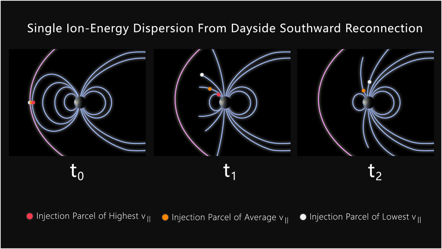
FIGURE 1. Ion-energy single dispersion process, which is well-understood. This process produces a single dispersed population, in contrast to the less understood double dispersion process that produces two dispersion populations, which we focus on in this work.

Previous studies of dispersion events established the groundwork for the analysis of the dispersion structure. In Lockwood and Smith (1992), it was shown that the slope of the dispersion in the spectrogram could be related to the upstream reconnection rate at the magnetopause. Wing et al. (2001) utilized modeling techniques to show that the double cusp structure can be predicted as a result of the differences in the $\vec{E}\times \vec{B}$ structure during strongly duskward/dawnward and weakly southward IMFs. Later in Trattner et al. (2015), dispersion signatures were used to distinguish between pulsed and continuous reconnections at the dayside magnetopause.

Cusp ion dispersions sometimes show overlapping signatures (Trattner et al. 1998; Trattner et al. 2012a). The leading interpretation has since become that multiple reconnection sites formed during the reconnection process generate this effect, wherein each simultaneous reconnection is responsible for a single injection (Lockwood, 1995). This is particularly because, in overlapping dispersion, the delay between each injection happens on a timescale understood to be significantly shorter than the accepted cadence of magnetically disjointed individual injections. This warrants a link to multiple reconnections, wherein the two injections are magnetically coupled, originating from the same global phenomenon and creating double injections very close to each other in time. Observationally, this is supported by direct measurements from the MMS era, which linked multiple reconnections to flux transfer events and the subsequent detection of overlapping dispersion in the cusp using MMS (Fuselier et al., 2018). More recently, direct measurements reported in Fuselier et al. (2022) observed multiple reconnection sites on the magnetopause with MMS and then, several hours later (during similar IMF conditions), double dispersion at the northern cusp with the Twin Rocket Investigation of Cusp Electrodynamics-2 (TRICE-2) rocket experiment.

Figure 2 shows an example of overlapping dispersion signatures in LEO (specifically 840–860 km) taken from the F-16 Satellite of the Defense Meteorological Satellite Program (DMSP) (Dickinson, 1974; Redmann, 1985). During this time, the satellite observes two plasma populations, where each of them displays energy dispersions (sorted over space by energy). This takes place between 10:13:00 UTC and 10:14:30 UTC. The key feature of this plot is that the central energy of each population decreases in energy with the increasing magnetic latitude. The satellite crosses the cusp region at a magnetic local time (MLT) of approximately 13.5 and magnetic latitudes (MLAT) between 74° and 77°.

FIGURE 2

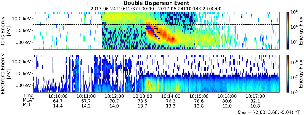
FIGURE 2. Example of a double dispersion event, acquired from the DMSP F-16 satellite. The top spectrogram illustrates the double dispersion occurring between 10:13:00 and 10:14:30. The satellite crosses through the two injections in the dayside northern cusp when the magnetic local time (MLT) is ≈13.5 h and the magnetic latitudes (MLAT) are between 74° and 77°. The blue line on top of the first dispersion population highlights their peak fluxes. Similarly, the black line emphasizes the peak flux of the second population during a period of overlap with the first population.

The contributions of this paper include extensions to the existing methodology and the use of these new techniques to observe statistical correlations. When we apply the methodology, we produce quantitative statistics of double dispersion in the dayside northern cusp during southward IMF. In the methodology section, we extend the algorithm developed in da Silva et al. (2022), originally for the automatic detection of single dispersion events. The algorithm is extended to detect double dispersion using the same general approach. We apply our new algorithm to the time period between January 2011 and August 2022. We report the number of detected double dispersion events with respect to the month of the year, the three IMF components (B_x, B_y, and B_z), and the IMF clock and cone angles. The relevant background to place each relationship in the proper context is reviewed, and the different ways to interpret the data are discussed.

In Section 2, we describe the DMSP mission, its associated instrument used to measure particle precipitation, and the OMNI dataset used for IMF measurements. In Section 3, we describe the new features implemented in our previously established single dispersion algorithm to enable double dispersion detection. Section 4 describes the preparation and hand review process conducted to remove false positives and curate the dataset quality. In Section 5, we present the findings of the rate with respect to the aforementioned variables. Finally, in Section 6, we review the contributions of this work and the progress made toward understanding double dispersion.

2 Data

In this study, we utilize data from the F-16 satellite of the DMSP mission (Dickinson, 1974; Redmann, 1985). Overall, the DMSP mission provides four decades of coverage of precipitating plasma data, acquired by multiple spacecraft in flight at any given time. DMSP utilizes a mission design wherein multiple spacecraft are placed in different LEOs and Sun-synchronous orbits, and a replacement strategy is used to ensure continuous coverage when a satellite reaches its end-of-life. We utilize data from the F-16 satellite (launched in 2003) because we found that the F-16 satellite provides more distinct dispersed cusp particle precipitation signatures. The F-16 satellite has an orbital period of 101 min, an inclination of 98.9°, and a nominal local time of ascending/descending nodes of 19:54/07:54.

The DMSP spacecraft includes top-facing electron and ion instruments with a 90° field of view, known as Special Sensor J (SSJ) instruments (Redmon et al., 2017). Because they are top-facing, the spectrograms measure only downward precipitating particles, excluding particles traveling upward due to the bounce motion. The SSJ instrument used in this study is of the fifth generation, known as SSJ/5, and comprises 16 log-spaced energies between 30 eV and 30 keV (similar to the previous generation SSJ/4, described in Hardy (1984)). In this study, we utilize the ion and electron differential energy flux data in units of eVcm⁻²s⁻¹sr⁻¹eV⁻¹.

In addition to the ion and electron differential energy flux data from SSJ/5, we also utilize estimates of IMF at the bow shock provided by the OMNI dataset (Papitashvili et al., 2014). OMNI provides high-resolution (1-min cadence) estimates of the IMF vector, solar wind velocity, and solar wind density. These variables are measured in situ at L₁ and are subsequently propagated to the bow shock during post-processing for magnetospheric applications (Chiu et al., 1998; Ogilvie et al., 1995;Ogilvie and Desch, 1997).

3 Methods

The methodology for automatically detecting double dispersion is built upon the previous work to detect single dispersion (da Silva et al., 2022). Here, we define a numerical criterion which is used to detect events. We begin with modeling the criteria around single dispersion events and then generalizing them to double dispersion events.

The modeling approach focuses on simplifying a spectrogram problem into a time series problem. This is carried out by characterizing an entire energy spread into a single time series variable E_p(t), where the variable’s value is located at the energy of peak flux (“p” stands for peak). Through this simplification, the problem of identifying a single dispersion curve becomes about characterizing patterns in one variable.

Our approach moves a sliding window through time, calculating an instantaneous score at each point in time. When the total score over a window is above a threshold, we mark that window as having an event. The equation for the selection criteria for single dispersion is then generally written as follows:

${\int }_{\mathit{window}}D\left(t\right)dt>\tau ,(1)$

where D(t) is the instantaneous scoring function and τ is the threshold. The threshold τ is itself a type of sensitivity, wherein lower thresholds are stricter and select fewer events. The scoring function is given by the following expression:

$D\left(t\right)=-\mathrm{sgn}\left(\frac{d|MLAT|}{dt}\right)\left[\frac{d{\left[\mathrm{L}\mathrm{o}\mathrm{g}E\right]}_{\mathit{smoothed}}}{dt}\right]b_{\mathit{south}}\left(t\right)e\left(t\right)g\left(t\right),(2)$

where MLAT is the magnetic latitude, b_south(t) has a value of 1 when B_z <0 (zero otherwise), e(t) has a value of 1 on the dayside (zero otherwise), and g(t) has a value of 1 when MLAT >50° (zero otherwise). The term $\frac{d{[\mathrm{L}\mathrm{o}\mathrm{g}E]}_{\mathit{smoothed}}}{dt}$ is used to tie the score to log-scale changes in E(t). The term $-\mathrm{sgn}\left(\frac{d|MLAT|}{dt}\right)$ is used to tie this change to the north–south vs. south–north path of the satellite, and overall produces a positive score when the pattern is indicative of southward IMF dispersion on the dayside. The variable [LogE]_smoothed is obtained by smoothing E(t) using a box-car averaging scheme with five points on each side. A window size of 60 s is used.

To generalize it to double dispersion, we use dual peak-finding methods to find two nominal energy curves, E_p1(t) and E_p2(t). A bimodal energy curve is illustrated in Figure 3. The criteria in Equation 1 are then generalized to the following:

${\int }_{\mathit{window}}{D}_{p1}\left(t\right)dt>\tau \mathrm{and}{\int }_{\mathit{window}}{D}_{p2}\left(t\right)dt>\tau ,(3)$

where D_p1(t) corresponds to E_p1(t) and D_p2(t) corresponds to E_p2(t). Details of the peak-finding and peak-labeling processes are subtle and complex; the full details are disclosed for those interested in the Appendix.

FIGURE 3

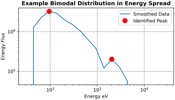
FIGURE 3. Example of energy spread at a single time step from DMSP SSJ/5 data, displaying a clean bimodal distribution over energy after the data are smoothed. A red dot is drawn at each of the identified peaks using our method.

Because double dispersion events are much rarer, finding a large set of hand-picked examples to validate against was not feasible. Four events were hand-picked from a study of the 20 December 2015 storm, and the algorithm was tuned until it was able to autonomously select all of them.

4 Double dispersion dataset

The automated double dispersion detection algorithm was run over the period of January 2011 and August 2022 using the DMSP F-16 satellite, with the intention of covering approximately one solar cycle. As outlined in Section 3, our search is confined to the northern cusp on the dayside and B_z <0. Following the automated selection of events, the detections were individually reviewed by hand and detections identified as double dispersions that were not real events (false positives) were filtered out. After this review process, the final collection resulted in a total of 138 events.

In particular, during the review process, we searched for events that met the following qualitative criteria:

1) The event showed two clear populations dispersed in ion energy over the magnetic latitude.

2) The event showed at least a partial overlap between the two dispersion populations.

3) The ion energy dispersion occurred at the same time as an increased flux of electrons.

In this collection of events, we discard those cases with double injections that (a) do not show dispersion features or (b) do not present an overlap. Non-overlapping injections are more consistent with the double cusp model developed in Wing et al. (2001), where $\vec{E}\times \vec{B}$ drift causes particles to arrive at two distinct locations.

Figure 4 shows the coverage of the satellite in magnetic coordinates over the time period studied. We identify two features which should be considered in the subsequent statistical report: (a) the coverage in the magnetic local time is not symmetric across noon, and the regions closer to dusk are more sampled than those close to dawn, and (b) the magnetic latitudes under 60° are similarly sampled closer to dusk. According to the cusp location model of Petrinec et al. (2023), compiled from published studies and applied to the recent TRICE-2 campaign of cusp region observations during southward IMF, the cusp is (a) centered at 12.6 h when B_y = 0, (b) moves duskward with increasing B_y (by a MLT factor of approximately 0.120 h/nT), (c) has a full extent of 6 h, and (d) has a magnetic latitude extent of 21.7 exp (0.1 B_z) + 58.2 + ψ/15 ± 1.00°, where ψ is the dipole tilt in degrees.

FIGURE 4

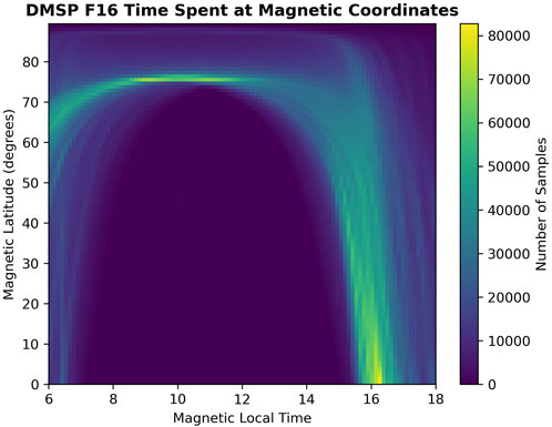
FIGURE 4. Coverage of the DMSP F-16 satellite in magnetic coordinates throughout the dataset studied. This plot should be consulted for considerations of the orbital bias. The bin sizes used in this plot are 0.01 h in the magnetic local time and 0.1° in the magnetic latitude.

The selected events are made available as both plots and a list of start/stop times in a computer-readable comma-separated value (CSV) format. Readers who wish to compare their understanding of the aforementioned criteria with the final selections may download the events to find the examples. The software application is also made available to repeat the initial search, with the option available to modify parameters, thresholds, and the core algorithm itself. Links to these can be found at the end of this paper.

5 Statistical report and discussion

The results collected from the previous section were organized to compare the detected event distributions as a function of various parameters. In particular, we focused on the detection rate with respect to the month of the year; the IMF components B_x, B_y, and B_z as provided by OMNI; and the IMF clock and cone angles.

5.1 Seasonal distribution of double dispersion events

The relationship between the number of detected events and the month of the year and the dipole tilt is shown in Figure 5. The month-of-the-year dependence reflects the average dipole tilt variability; during the northern hemisphere summer, the dipole is primarily tilted toward the Sun, and during the northern hemisphere winter, the dipole is primarily tilted away from the Sun.

FIGURE 5

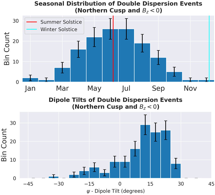
FIGURE 5. Seasonal month-by-month and dipole tilt distributions of hand-validated double dispersion events in the northern cusp, which show a strong preference for events during the summer months and high-dipole tilts. During the summer months, Earth’s dipole is tilted toward the Sun. The error bars displayed on the histogram bars correspond to the 1σ error inferred from Poisson counting statistics (${\sigma }_i\approx \sqrt{H_i}$, where H_i is the bin count for bin i) and are meant to give a ballpark scale of the error associated with our sample size and binning.

The dependence on dipole tilt is put in context with other correlations among the dipole tilt, the cusp, and magnetic reconnection. First, we look at the preferred location of the x-line dictated by non-multiple reconnection models as this should be considered when preparing interpretations about the multiple reconnection formation process (Fu and Lee, 1985; Lee and Fu, 1985). It is determined by the observation-derived Maximum Magnetic Shear (MaxMS) model, which states that increasing the dipole tilt will move the x-line southward on the magnetopause (Fuselier et al., 2021; Trattner et al. 2012b; Trattner et al. 2017; Trattner et al. 2021). This is supported by MHD simulations of the dipole tilt effect on magnetic reconnection during B_z south (Eggington et al., 2020). Related to this are remote-sensing imaging observations of energetic neutral atoms (ENAs) in the cusps. ENAs, which are often but not always caused by participle precipitation, show an increased flux in the northern cusp during the summer months, as well as an asymmetric increase in the flux in the southern cusp during the northern hemisphere winter (Petrinec et al., 2011). This is relevant because increased ENA signatures are indicative (although not completely conclusively indicative) of increased precipitation (Fear et al. (2012); Raeder (2006)).

5.2 IMF distribution of double dispersion events

Figure 6 shows the relationship between the number of detected events and the IMF $\vec{B}$ components provided by OMNI at the time of each event, normalized to all IMF conditions (i.e., the distribution of $\vec{B}$ components over the full period).

FIGURE 6

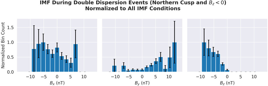
FIGURE 6. IMF component values during each of the detected events from the northern cusp during B_z <0, normalized to all IMF conditions. These coordinates are in the GSM coordinate system. This plot indicates a noticeably higher number of detected events when (a) IMF has a positive B_y component and (b) when B_z is more negative. The error bars displayed on the histogram correspond to the 1σ error inferred from Poisson counting statistics (${\sigma }_i\approx \alpha \sqrt{H_i}$, where H_i is the bin count for bin i and α is the normalization scale factor) and is meant to give a ballpark scale of the error associated with our sample size and binning.

The strongest features of this plot are the higher normalized bin counts for events during B_y >0, generally increasing with a more positive B_y value. Although the normalized bin count increases with a more positive B_y value, there is a drop of approximately 7 nT before the final bin with a large error bar (this was a single detection scaled by normalization). The preference for positive B_y will be displayed later in terms of IMF clock and cone angles.

We also note that there is a preference for B_y-dominant IMFs. Out of all the detected events, 68% occur during B_y-dominant IMFs, compared to 34% of all IMF conditions with B_y being dominant. Within the subset of detections where B_y >0, 88% occur during B_y-dominant IMFs, compared to 60% of all IMF conditions, which are B_y >0.

We must also consider whether the orbit of the satellite has an impact on the observed preference for positive B_y. The structure of the time spent at each magnetic coordinate, shown in Figure 4, combined with the cusp location model of Petrinec et al. (2023), indicates the satellite over the sample cusp locations for a positive B_y. We are, therefore, unable to definitely conclude whether this bias contributes to exaggerating the preference for B_y, or whether this bias generates a false appearance of a preference altogether.

We constrained the search to B_z <0 specifically, so we necessarily only observe that range here. We see that the normalized bin count increases with a more negative B_z value.

According to the Russell–McPherron effect, southward IMFs preferentially occur for several weeks surrounding the autumn equinox for B_y >0. In contrast, southward IMFs preferentially occur for several weeks surrounding the vernal equinox for B_y <0. However, as seen in Figure 5, there are fewer events from March to May than from July to September. This could be an explanation for why B_y is asymmetric toward B_y >0. IMF is also statistically oriented along the Parker spiral angle, favoring cases with B_y >0 and B_x <0 or B_y <0 and B_x >0. From this general distribution, an asymmetry toward B_y >0 should also include a weaker but still significant asymmetry toward B_x <0, which is seen in Figure 6.

5.3 IMF clock and cone angle distributions of double dispersion events

The IMF clock and cone angles are the most fundamental inputs into the magnetosphere when it comes to particle precipitation and magnetic reconnection. We also report the relationship between the normalized bin counts and the IMF clock and cone angles (Figure 7). We compute the IMF clock angle θ_clock as the angle $\vec{B}$ makes with the GSM $\widehat{z}$ axis when projected on the B_y/B_z plane (Cheng et al., 2013) and the IMF cone angle as the angle between $B_x\widehat{x}$ and $\vec{B}$. All coordinates are in the GSM coordinate system. To allow for values of θ_clock between −180° and 180° instead of −90° and 90°, we then use a two argument function tan⁻¹(B_y, B_z) instead of tan⁻¹(B_y/B_z) as it considers the direction of the angle separately as to whether it opens from the left or right. This two-argument version is sometimes called arctan2 or atan2.

FIGURE 7

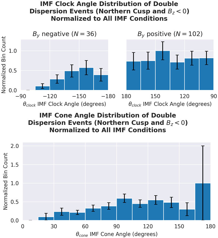
FIGURE 7. Distribution of the IMF clock and cone angles over the detected double dispersion events, normalized to account for all IMF conditions and a spherical geometry consideration. The spherical geometry consideration is the normalization to sin(θ_cone). The IMF data are taken from OMNI, which is derived from the L₁ in situ satellite measurements propagated to the bow shock for magnetospheric applications. We note that θ =−180° and θ =180° correspond to the same clock angle.

The equations used to compute the clock and cone angles are as follows:

${\theta }_{\mathit{clock}}={\tan }^{-1}\left(B_y,B_z\right)(4)$

and

${\theta }_{\mathit{cone}}={\cos }^{-1}\left(B_x/B\right).(5)$

The distribution of cone angles is normalized to the overall occurrence of IMF and sin (θ_cone) to account for the bias of the subtended area of the unit sphere covered by each cone angle (consider in this analogy that there is less area on Earth between 80° and 85° latitude than that between −5° and +5° latitude). The error bars are updated to reflect this normalization.

The higher normalized bin counts for positive B_y are visible in the relationship with the clock angle as well. It is noticed that all normalized bin counts for clock angles corresponding to B_y are roughly within the error bars of each other, showing no strong preference for one positive B_y clock angle over others.

The cone angle is related to whether component reconnection or anti-parallel reconnection is occurring in Trattner et al. (2021). When the cone angle is very small or very large (θ_cone <45° or θ_cone >135°), an anti-parallel reconnection occurs; otherwise, component reconnection occurs. In the clock angle distribution seen here, only 23 out of the 138 events correspond to anti-parallel reconnection, suggesting that double dispersion is more likely to occur during component reconnection.

The IMF clock angle is understood to be a critical variable in the study of global magnetospheric reconnection. For example, higher clock angles (anti-parallel reconnection) correspond to increased reconnection rates (Scurry and Russell, 1991). In terms of the reconnection geometry, global simulations have found a dependence on the location of magnetic separators with the IMF clock angle (Komar et al., 2013). In particular, it was demonstrated that the surface in which the separator lies rotates around the Sun–Earth line as the clock angle increases. However, this study did not use a version of the clock angle spanning only 180°. In the context of multiple reconnections, a related study demonstrated that as the clock angle decreases, the corresponding flux ropes become tilted, relative to the equatorial plane, and increase in length (Guo et al., 2021).

An explanation for the cause of double dispersion should seek to integrate the previous literature on the relationship between the IMF clock/cone angles and magnetic reconnection geometry. Several questions about double dispersion, such as whether multiple reconnection sites inject their particles simultaneously with a delay, may be explored using reconnection geometry and considerations of the time of flight, as observed in situ. This can narrow the range of the possible explanations by de-emphasizing explanations inconsistent with reconnection geometries associated with the clock angle distributions reported here (Schwenn, 2007; Tokumaru et al., 2010; Bame et al., 1976).

6 Conclusion

In this work, we presented the first statistical report of double dispersion, a term used here to mean overlapping double-injection ion-energy dispersion events in the cusps. An algorithm previously established in the literature for single-injection dispersion was extended to automatically detect double dispersion, and the extensions were documented, justified, and applied here. We used an algorithm to narrow the number of events, which were also reviewed by hand according to the criteria stated in Section 4 to ensure scientific integrity.

Using our collection of events, we reported the statistics on relationships between the number of detected events and several other variables. The distributions explored include binning by the month of the year (seasonally) (5.1), the three IMF components (5.2), and the IMF clock and cone angles (5.3). The seasonal distribution indicated that the events were found much more during the summer months when the dipole was tilted toward the Sun, a finding that can be linked to the reconnection geometry. The distribution of three IMF components and the IMF clock angle indicated a preference for detection in response to a more positive B_y value, but we cannot say this conclusively due to the orbit of the DMSP F-16 satellite.

In this study, we looked at the northern cusp. This limitation was due to the orbit of the DMSP F-16 satellite we used. However, important questions relating to the seasonal bias reported here can be elevated by repeating the analysis for the southern cusp as well. Overall, the signature of double dispersion in the cusp presents a 2D picture (over energy and time) of the global reconnection process, which is necessarily 7D (over space, velocity, and time) in nature. The statistics reported in this paper are made possible due to the long lifetime of the DMSP F-16 satellite and the accessibility (in terms of the revisit rate) for cusp crossings in the low Earth orbit. As investigations into magnetic reconnection in the magnetosphere continue, double dispersion continues to provide us with a powerful perspective to understand these phenomena.

Data availability statement

Original datasets are available in a publicly accessible repository: The original contributions presented in the study are publicly available. This data can be found here: https://doi.org/10.5281/zenodo.10071944.

Author contributions

DS wrote the manuscript and performed the data analysis. The concept was developed by DS, LC, and KT. All authors contributed to the article and approved the submitted version.

Conflict of interest

Author SP was employed by the Lockheed Martin Advanced Technology Center.

The remaining authors declare that the research was conducted in the absence of any commercial or financial relationships that could be construed as a potential conflict of interest.

Publisher’s note

All claims expressed in this article are solely those of the authors and do not necessarily represent those of their affiliated organizations, or those of the publisher, the editors, and the reviewers. Any product that may be evaluated in this article, or claim that may be made by its manufacturer, is not guaranteed or endorsed by the publisher.

Supplementary material

The Supplementary Material for this article can be found online at: https://www.frontiersin.org/articles/10.3389/frsfm.2023.1281171/full#supplementary-material

References

Bame, S., Asbridge, J., Feldman, W., and Gosling, J. (1976). Solar cycle evolution of high-speed solar wind streams. Astrophysical J. 207, 977–980. doi:10.1086/154566

CrossRef Full Text | Google Scholar

Basinska, E. M., Burke, W. J., Maynard, N. C., Hughes, W., Winningham, J., and Hanson, W. (1992). Small-scale electrodynamics of the cusp with northward interplanetary magnetic field. J. Geophys. Res. Space Phys. 97, 6369–6379. doi:10.1029/91ja03023

CrossRef Full Text | Google Scholar

Burch, J., Moore, T., Torbert, R., and Giles, B. (2016a). Magnetospheric multiscale overview and science objectives. Space Sci. Rev. 199, 5–21. doi:10.1007/s11214-015-0164-9

CrossRef Full Text | Google Scholar

Burch, J., Reiff, P., Heelis, R., Winningham, J., Hanson, W., Gurgiolo, C., et al. (1982). Plasma injection and transport in the mid-altitude polar cusp. Geophys. Res. Lett. 9, 921–924. doi:10.1029/gl009i009p00921

CrossRef Full Text | Google Scholar

Burch, J., Torbert, R., Phan, T., Chen, L.-J., Moore, T., Ergun, R., et al. (2016b). Electron-scale measurements of magnetic reconnection in space. Science 352, aaf2939. doi:10.1126/science.aaf2939

PubMed Abstract | CrossRef Full Text | Google Scholar

Burkholder, B. L., Chen, L.-J., Fuselier, S., Gershman, D., Schiff, C., Shuster, J., et al. (2022). MMS observations of storm-time magnetopause boundary layers in the vicinity of the southern cusp. Geophys. Res. Lett. 49. doi:10.1029/2022gl101231

CrossRef Full Text | Google Scholar

Cheng, Z., Shi, J., Dunlop, M., and Liu, Z. (2013). Influences of the interplanetary magnetic field clock angle and cone angle on the field-aligned currents in the magnetotail. Geophys. Res. Lett. 40, 5355–5359. doi:10.1002/2013gl056737

CrossRef Full Text | Google Scholar

Chiu, M., Von-Mehlem, U., Willey, C., Betenbaugh, T., Maynard, J., Krein, J., et al. (1998). ACE spacecraft. Space Sci. Rev. 86, 257–284. doi:10.1023/a:1005002013459

CrossRef Full Text | Google Scholar

da Silva, D., Chen, L., Fuselier, S., Wang, S., Elkington, S., Dorelli, J., et al. (2022). Automatic identification and new observations of ion energy dispersion events in the cusp ionosphere. J. Geophys. Res. Space Phys. 127, e2021JA029637. doi:10.1029/2021ja029637

CrossRef Full Text | Google Scholar

Dickinson, L. G. (1974). Defense meteorological satellite program (DMSP) user’s guide, vol. 74 (AWS).

Google Scholar

Dunlop, M., Zhang, Q.-H., Bogdanova, Y., Trattner, K., Pu, Z., Hasegawa, H., et al. (2011). Magnetopause reconnection across wide local time. Ann. Geophys. Copernic. GmbH) 29, 1683–1697. doi:10.5194/angeo-29-1683-2011

CrossRef Full Text | Google Scholar

Eggington, J., Eastwood, J., Mejnertsen, L., Desai, R., and Chittenden, J. (2020). Dipole tilt effect on magnetopause reconnection and the steady-state magnetosphere-ionosphere system: global mhd simulations. J. Geophys. Res. Space Phys. 125, e2019JA027510. doi:10.1029/2019ja027510

CrossRef Full Text | Google Scholar

Escoubet, C., Fehringer, M., and Goldstein, M. (2001). Introduction the cluster mission. Ann. Geophys. Copernic. GmbH) 19, 1197–1200. doi:10.5194/angeo-19-1197-2001

CrossRef Full Text | Google Scholar

Fear, R., Palmroth, M., and Milan, S. (2012). Seasonal and clock angle control of the location of flux transfer event signatures at the magnetopause. J. Geophys. Res. Space Phys. 117. doi:10.1029/2011ja017235

CrossRef Full Text | Google Scholar

Frank, L., and Craven, J. (1988). Imaging results from dynamics explorer 1. Rev. Geophys. 26, 249–283. doi:10.1029/rg026i002p00249

CrossRef Full Text | Google Scholar

Frey, H. U., Han, D., Kataoka, R., Lessard, M. R., Milan, S. E., Nishimura, Y., et al. (2019). Dayside aurora. Space Sci. Rev. 215, 51–32. doi:10.1007/s11214-019-0617-7

CrossRef Full Text | Google Scholar

Frey, S., Angelopoulos, V., Bester, M., Bonnell, J., Phan, T., and Rummel, D. (2008). Orbit design for the themis mission. Space Sci. Rev. 141, 61–89. doi:10.1007/s11214-008-9441-1

CrossRef Full Text | Google Scholar

Fu, Z., and Lee, L. (1985). Simulation of multiple x-line reconnection at the dayside magnetopause. Geophys. Res. Lett. 12, 291–294. doi:10.1029/gl012i005p00291

CrossRef Full Text | Google Scholar

Fuselier, S., Kletzing, C., Petrinec, S., Trattner, K., George, D., Bounds, S., et al. (2022). Multiple reconnection x-lines at the magnetopause and overlapping cusp ion injections. J. Geophys. Res. Space Phys. 127. e2022JA030354. doi:10.1029/2022ja030354

CrossRef Full Text | Google Scholar

Fuselier, S., Lewis, W., Schiff, C., Ergun, R., Burch, J., Petrinec, S., et al. (2016). Magnetospheric multiscale science mission profile and operations. Space Sci. Rev. 199, 77–103. doi:10.1007/s11214-014-0087-x

CrossRef Full Text | Google Scholar

Fuselier, S., Petrinec, S., Trattner, K. J., Broll, J., Burch, J., Giles, B., et al. (2018). Observational evidence of large-scale multiple reconnection at the earth’s dayside magnetopause. J. Geophys. Res. Space Phys. 123, 8407–8421. doi:10.1029/2018ja025681

CrossRef Full Text | Google Scholar

Fuselier, S. A., Webster, J., Trattner, K. J., Petrinec, S., Genestreti, K. J., Pritchard, K. R., et al. (2021). Reconnection x-line orientations at the earth’s magnetopause. J. Geophys. Res. Space Phys. 126, e2021JA029789. doi:10.1029/2021ja029789

CrossRef Full Text | Google Scholar

Guo, J., Lu, S., Lu, Q., Lin, Y., Wang, X., Huang, K., et al. (2021). Structure and coalescence of magnetopause flux ropes and their dependence on IMF clock angle: three-dimensional global hybrid simulations. J. Geophys. Res. Space Phys. 126, e2020JA028670. doi:10.1029/2020ja028670

CrossRef Full Text | Google Scholar

Hardy, D. A. (1984). Precipitating electron and ion detectors (ssj/4) for the block 5d/flights 6-10 DMSP satellites: calibration and data presentation. AFGL-TR-84-0317.

Google Scholar

Komar, C., Cassak, P., Dorelli, J., Glocer, A., and Kuznetsova, M. (2013). Tracing magnetic separators and their dependence on IMF clock angle in global magnetospheric simulations. J. Geophys. Res. Space Phys. 118, 4998–5007. doi:10.1002/jgra.50479

CrossRef Full Text | Google Scholar

Lavraud, B., and Trattner, K. J. (2021). The polar cusps of the earth’s magnetosphere. Magnetos. Sol. Syst., 163–176. doi:10.1002/9781119815624.ch11

CrossRef Full Text | Google Scholar

Lee, L., and Fu, Z. (1985). A theory of magnetic flux transfer at the earth’s magnetopause. Geophys. Res. Lett. 12, 105–108. doi:10.1029/gl012i002p00105

CrossRef Full Text | Google Scholar

Lockwood, M. (1995). Overlapping cusp ion injections: an explanation invoking magnetopause reconnection. Geophys. Res. Lett. 22, 1141–1144. doi:10.1029/95gl00811

CrossRef Full Text | Google Scholar

Lockwood, M., and Smith, M. (1992). The variation of reconnection rate at the dayside magnetopause and cusp ion precipitation. J. Geophys. Res. Space Phys. 97, 14841–14847. doi:10.1029/92ja01261

CrossRef Full Text | Google Scholar

Lockwood, M., and Smith, M. (1994). Low and middle altitude cusp particle signatures for general magnetopause reconnection rate variations: 1. theory. J. Geophys. Res. Space Phys. 99, 8531–8553. doi:10.1029/93ja03399

CrossRef Full Text | Google Scholar

Lockwood, M., and Smith, M. F. (1989). Low-altitude signatures of the cusp and flux transfer events. Geophys. Res. Lett. 16, 879–882. doi:10.1029/gl016i008p00879

CrossRef Full Text | Google Scholar

Nishida, A. (1994). The GEOTAIL mission.

Google Scholar

Ogilvie, K., Chornay, D., Fritzenreiter, R., Hunsaker, F., Keller, J., Lobell, J., et al. (1995). SWE, a comprehensive plasma instrument for the WIND spacecraft. Space Sci. Rev. 71, 55–77. doi:10.1007/bf00751326

CrossRef Full Text | Google Scholar

Ogilvie, K., and Desch, M. (1997). The WIND spacecraft and its early scientific results. Adv. Space Res. 20, 559–568. doi:10.1016/s0273-1177(97)00439-0

CrossRef Full Text | Google Scholar

Papitashvili, N., Bilitza, D., and King, J. (2014). Omni: a description of near-earth solar wind environment. 40th COSPAR Sci. Assem. 40. C0–1.

Google Scholar

Paschmann, G., Sonnerup, B. Ö., Papamastorakis, I., Sckopke, N., Haerendel, G., Bame, S., et al. (1979). Plasma acceleration at the earth’s magnetopause: evidence for reconnection. Nature 282, 243–246. doi:10.1038/282243a0

CrossRef Full Text | Google Scholar

Petrinec, S., Dayeh, M., Funsten, H., Fuselier, S., Heirtzler, D., Janzen, P., et al. (2011). Neutral atom imaging of the magnetospheric cusps. J. Geophys. Res. Space Phys. 116. doi:10.1029/2010ja016357

CrossRef Full Text | Google Scholar

Petrinec, S., Kletzing, C., Bounds, S., Fuselier, S., Trattner, K., and Sawyer, R. (2023). TRICE-2 rocket observations in the low-altitude cusp: boundaries and comparisons with models. J. Geophys. Res. Space Phys. 128. e2022JA030952. doi:10.1029/2022ja030952

CrossRef Full Text | Google Scholar

Pitout, F., and Bogdanova, Y. (2021). The polar cusp seen by cluster. J. Geophys. Res. Space Phys. 126, e2021JA029582. doi:10.1029/2021ja029582

CrossRef Full Text | Google Scholar

Raeder, J. (2006). “Flux transfer events: 1. generation mechanism for strong southward imf,” in Annales geophysicae (Copernicus Publications Göttingen, Germany), 24, 381–392.

CrossRef Full Text | Google Scholar

Redmann, J. (1985). An overview of the mission sensor systems of the dmsp satellites. In 23rd Aerospace Sciences Meeting. 240.

CrossRef Full Text | Google Scholar

Redmon, R. J., Denig, W. F., Kilcommons, L. M., and Knipp, D. J. (2017). New DMSP database of precipitating auroral electrons and ions. J. Geophys. Res. Space Phys. 122, 9056–9067. doi:10.1002/2016ja023339

PubMed Abstract | CrossRef Full Text | Google Scholar

Reiff, P., Hill, T., and Burch, J. (1977). Solar wind plasma injection at the dayside magnetospheric cusp. J. Geophys. Res. 82, 479–491. doi:10.1029/ja082i004p00479

CrossRef Full Text | Google Scholar

Retinò, A., Vaivads, A., André, M., Sahraoui, F., Khotyaintsev, Y., Pickett, J., et al. (2006). Structure of the separatrix region close to a magnetic reconnection x-line: cluster observations. Geophys. Res. Lett. 33, L06101. doi:10.1029/2005gl024650

CrossRef Full Text | Google Scholar

Russell, C. T., and Elphic, R. (1978). Initial ISEE magnetometer results: magnetopause observations. Space Sci. Rev. 22, 681–715. doi:10.1007/bf00212619

CrossRef Full Text | Google Scholar

Schwenn, R. (2007). Solar wind sources and their variations over the solar cycle. Sol. Dyn. its Eff. heliosphere Earth, 51–76. doi:10.1007/978-0-387-69532-7_5

CrossRef Full Text | Google Scholar

Scurry, L., and Russell, C. (1991). Proxy studies of energy transfer to the magnetosphere. J. Geophys. Res. Space Phys. 96, 9541–9548. doi:10.1029/91ja00569

CrossRef Full Text | Google Scholar

Sibeck, D., and Angelopoulos, V. (2008). THEMIS science objectives and mission phases. Space Sci. Rev. 141, 35–59. doi:10.1007/s11214-008-9393-5

CrossRef Full Text | Google Scholar

Sonnerup, B. Ö., Paschmann, G., Papamastorakis, I., Sckopke, N., Haerendel, G., Bame, S., et al. (1981). Evidence for magnetic field reconnection at the earth’s magnetopause. J. Geophys. Res. Space Phys. 86, 10049–10067. doi:10.1029/ja086ia12p10049

CrossRef Full Text | Google Scholar

Tokumaru, M., Kojima, M., and Fujiki, K. (2010). Solar cycle evolution of the solar wind speed distribution from 1985 to 2008. J. Geophys. Res. Space Phys. 115. doi:10.1029/2009ja014628

CrossRef Full Text | Google Scholar

Trattner, K., Burch, J., Ergun, R., Eriksson, S., Fuselier, S., Giles, B., et al. (2017). The MMS dayside magnetic reconnection locations during phase 1 and their relation to the predictions of the maximum magnetic shear model. J. Geophys. Res. Space Phys. 122, 11–991. doi:10.1002/2017ja024488

CrossRef Full Text | Google Scholar

Trattner, K., Coates, A., Fazakerley, A., Johnstone, A., Balsiger, H., Burch, J., et al. (1998). Overlapping ion populations in the cusp: polar/TIMAS results. Geophys. Res. Lett. 25, 1621–1624. doi:10.1029/98gl01060

CrossRef Full Text | Google Scholar

Trattner, K., Onsager, T., Petrinec, S., and Fuselier, S. (2015). Distinguishing between pulsed and continuous reconnection at the dayside magnetopause. J. Geophys. Res. Space Phys. 120, 1684–1696. doi:10.1002/2014ja020713

PubMed Abstract | CrossRef Full Text | Google Scholar

Trattner, K., Petrinec, S., and Fuselier, S. (2021). The location of magnetic reconnection at earth’s magnetopause. Space Sci. Rev. 217, 41. doi:10.1007/s11214-021-00817-8

PubMed Abstract | CrossRef Full Text | Google Scholar

Trattner, K., Petrinec, S., Fuselier, S., Omidi, N., and Sibeck, D. G. (2012a). Evidence of multiple reconnection lines at the magnetopause from cusp observations. J. Geophys. Res. Space Phys. 117. doi:10.1029/2011ja017080

CrossRef Full Text | Google Scholar

Trattner, K., Petrinec, S., Fuselier, S., and Phan, T. (2012b). The location of reconnection at the magnetopause: testing the maximum magnetic shear model with themis observations. J. Geophys. Res. Space Phys. 117. doi:10.1029/2011ja016959

CrossRef Full Text | Google Scholar

Virtanen, P., Gommers, R., Oliphant, T. E., Haberland, M., Reddy, T., Cournapeau, D., et al. (2020). SciPy 1.0: fundamental algorithms for scientific computing in python. Nat. methods 17, 261–272. doi:10.1038/s41592-019-0686-2

PubMed Abstract | CrossRef Full Text | Google Scholar

Wing, S., Newell, P. T., and Ruohoniemi, J. M. (2001). Double cusp: model prediction and observational verification. J. Geophys. Res. Space Phys. 106, 25571–25593. doi:10.1029/2000ja000402

CrossRef Full Text | Google Scholar

Appendix: Peak-finding and peak-labeling algorithm

In this section, we describe the process of analyzing an instantaneous energy spread to identify and label both peaks. The process is deceptively difficult as once one or two peaks are identified, each must be labeled correctly as “peak 1” or “peak 2” in a way that is self-consistent throughout time.

First, the energy spread is smoothed with a Savitzky–Golay filter. This filter uses a 5-point window and second-order polynomials. This is carried out to prevent noise from interfering with the peak-finding process.

The peak-finding process is performed at each time step with the find_peaks() function in SciPy (Virtanen et al., 2020). The function is configured to do a very simple search for energies whose flux is greater than both their immediate neighbors. Of the returned locations, we drop those that we do not want. We drop those which correspond to very low ion fluxes (threshold of 10^6.5 eVcm⁻²s⁻¹sr⁻¹eV⁻¹) as those are around the noise level. We also drop those which correspond to energies we do not associate with the magnetosheath (threshold of 10^3.5 eV). We note that this excludes magnetosheath particles which may be accelerated to super-magnetosheath energies (Burkholder et al., 2022).

If there are more than two locations returned, we use those with the top two highest fluxes. When we find two peaks, the labeling process is straightforward; we mark the one with a lower energy E_p1(t) and the other E_p2(t). The scenarios where we find one peak are more complicated.

When we find one peak, we must make a decision whether to assign the peak to E_p1 (t_i) or E_p2 (t_i), marking the other with a fill value. If the previous time step only found one peak, we immediately copy whatever label that was given to that, circumventing any further decision. If the previous step found two peaks, then we label the current peak as continuing E_p1(t), if and only if the current energy is lower than it. If the previous step did not find two peaks, then we continue E_p2(t) for lack of a better option.