- 1Cornell Center for Astrophysics and Planetary Science (CCAPS) and Department of Statistics and Data Science, Cornell University, Ithaca, NY, United States
- 2Department of Statistical Science, Duke University, Durham, NC, United States
Bayesian inference gets its name from Bayes’s theorem, expressing posterior probabilities for hypotheses about a data generating process as the (normalized) product of prior probabilities and a likelihood function. But Bayesian inference uses all of probability theory, not just Bayes’s theorem. Many hypotheses of scientific interest are composite hypotheses, with the strength of evidence for the hypothesis dependent on knowledge about auxiliary factors, such as the values of nuisance parameters (e.g., uncertain background rates or calibration factors). Many important capabilities of Bayesian methods arise from use of the law of total probability, which instructs analysts to compute probabilities for composite hypotheses by marginalization over auxiliary factors. This tutorial targets relative newcomers to Bayesian inference, aiming to complement tutorials that focus on Bayes’s theorem and how priors modulate likelihoods. The emphasis here is on marginalization over parameter spaces—both how it is the foundation for important capabilities, and how it may motivate caution when parameter spaces are large. Topics covered include the difference between likelihood and probability, understanding the impact of priors beyond merely shifting the maximum likelihood estimate, and the role of marginalization in accounting for uncertainty in nuisance parameters, systematic error, and model misspecification.
1 Introduction
The Bayesian approach to statistical inference and other data analysis tasks gets its name from Bayes’s theorem (BT). BT specifies that a posterior probability for a hypothesis concerning a data generating process may be computed by multiplying a prior probability and a likelihood function (and normalizing):
Tutorials on Bayesian methods often focus on how BT adjusts the likelihood function to account for base rates of hypotheses about members of a population, using simple examples like binary classification (e.g., disease/no-disease; guilty/not-guilty; star/galaxy) based on binary diagnostic data (e.g., a positive or negative test or evidentiary result). At the iid 2022: Statistical Methods for Event Data meeting that is the topic of this special issue of Frontiers, a charming and insightful tutorial along these lines was presented by Torsten Enßlin; see his “Bayes Basics” presentation at the meeting’s website.
In this tutorial contribution to the issue we address readers familiar with (and perhaps already using) Bayesian methods, to make the case that a focus on Bayes’s theorem risks overlooking a more fundamental and crucial aspect of Bayesian inference. We consider a key distinguishing feature of Bayesian inference to be is its use of the law of total probability (LTP), directing one to compute probabilities for composite hypotheses by marginalizing over the hypothesis or parameter space.
We do not consider this a new or controversial insight. The first author came to appreciate it as a student of the work of Jeffreys (1961), Jaynes (2003), Zellner (1971), and other mid-20th-century pioneers of modern Bayesian inference, and through the work of the second author and Jim Berger (Berger and Wolpert (1988), especially §§ 3.5 and 5.3). We have highlighted this in the past (e.g., in Loredo (1992; 1999; 2013); Berger et al. (1999), and in lectures at the Penn State Summer School in Statistics for Astronomers). But we feel this aspect of Bayesian analysis is underappreciated, especially by newcomers and non-experts. With the growing importance of high-dimensional models in statistics and machine learning (ML) there is new motivation for highlighting it. In particular, ML relies heavily on optimization over large parameter spaces, where, from a Bayesian perspective, marginalization may instead be the right operation. Recent research demonstrates that the performance of some ML models can be significantly enhanced by replacing optimization with marginalization (even approximately), particularly in settings were good uncertainty quantification is important. Andrew Wilson’s Bayesian machine learning group has done particularly notable work in this direction (Wilson, 2020; Wilson and Izmailov, 2020). It seems to us the crucial importance of the LTP and marginalization deserves amplification, particularly for newcomers to Bayesian methods.
In this tutorial, we start by establishing notation and informally reviewing BT, the LTP, and the Bayesian interpretation of probability. Then we explore the role of marginalization in Bayesian inference in the context of the following topics:
2 Notation and basic concepts
We adopt notation similar to that of Jeffreys, Cox, and Jaynes, who view Bayesian inference as a generalized logic (Cox, 1946; Jeffreys, 1961; Jaynes, 2003). Whereas deductive logic provides a calculus for truth and falsity in settings where we can reason with certainty (e.g., with truth and falsity represented by 1 and 0 in Boolean algebra), probability theory provides a calculus for degrees of entailment, or argument strength, in settings where we must quantify uncertainty (with probabilities taking values over the real interval, [0,1]). We use
We will often be computing a collection of probabilities that share common conditions that will not be questioned (i.e., they never appear to the left of the conditioning bar), at least for the duration of a specific calculation. We often denote such conditioning information by
Complex statements may be built by combining simpler statements. For example, we use
and the disjunction rule (the “or” or “sum” rule):
We presume the reader is familiar with these basics; they are here to establish notation and terminology.
We often compute probabilities for collections of statements labeled by an integer or a real-valued parameter (or vector of parameters). In such cases we use a lower-case
When conditioning information is common to all probability symbols in a formula it can be distracting to display it explicitly. We sometimes suppress symbols for common conditions for clarity, when the conditions are clear from the context. When we do want to display a common dependence, we adopt clever notation introduced by John Skilling (the “Skilling conditional”), showing the shared information with a double bar beside the equations, as here:
In what follows we will focus on Bayesian inference—computing probabilities for hypotheses of interest given data and other information, including modeling assumptions. Bayesian inference is the core of Bayesian data analysis (BDA), comprising the use of Bayesian probability for a broader variety of tasks, including making decisions (Bayesian decision theory), designing experiments (Bayesian experimental design), and addressing tasks where there is not enough structure for formal inference (e.g., Bayesian model checking and Bayesian exploratory data analysis). Marginalization plays a key role in all of these data analytical activities. The book Bayesian Data Analysis (Gelman et al., 2014a) provides comprehensive coverage of many topics comprising BDA. An emerging term of art, Bayesian workflow, refers to best practices for integrating diverse Bayesian techniques (including methods fusing Bayesian and frequentist considerations) into robust data analysis pipelines that include model checking and refinement steps. Gelman et al. (2020) provide a broad discussion of Bayesian workflow; Tak et al. (2018) and Eadie et al. (2023) discuss key components of sound Bayesian workflow in astrostatistics.
3 Bayes’s theorem and interpreting probability
If we equate the two factorizations on the right hand side of Equation 2 and solve for
provided that
To get BT in a form useful for data analysis, let
With these choices for the statements, the factors in this equation have names:
If we are considering a continuum of hypotheses labeled by a continuous parameter
(where we have mildly overloaded our notation, using
There is nothing controversial in BT as an uninterpreted mathematical result. But a problem arises in its use for data analysis if one insists on adopting a frequentist interpretation of probability. Such interpretations assert that probabilities can be meaningfully assigned and manipulated only for statements about quantities that take on diverse values in some kind of replication setting; such statements are called events3. In such settings, the probability for an event is the fraction of the time the event happens (the statement is true) among replications, as the number of replications tends to infinity4. The frequentist view is significantly restrictive. It allows us to say, “the probability for heads is
More importantly, the frequentist interpretation does not permit assigning or computing probabilities for hypotheses about fixed but uncertain properties of a physical system. For example, in the 1800s Laplace famously used Bayesian probability (the historically original notion of probability) to analyze detailed but noisy observations of Saturn’s orbit to estimate the ratio of Saturn’s mass to the Sun’s mass. He estimated the ratio to be within
One sometimes hears a complaint from a scientist only familiar with the frequentist interpretation that they can follow the Bayesian math, but stumble at the idea that a parameter value should be considered to be “random,” a random variable taking on a distribution of values. This reflects an error in interpretation. Figure 1 is our attempt at depicting the different interpretations for a PDF for some real-valued quantity

Figure 1. Frequentist and Bayesian interpretations of a PDF (blue curve) for a real-valued quantity
4 The law of total probability and marginalization
BT followed from the conjunction (“and”) rule. The LTP follows from application of both the conjunction and disjunction (“or”) rules to problems where a statement of interest may be true or false depending on what is true about auxiliary details in the problem. As simple example, consider rolling a die, and a hypothesis about the outcome of a single roll,
In such settings, the joint probability (“and”) for
where for the final equation we used repeated application of the “or” rule and the suite property to show that
where the last line uses the alternative factorization of
First, if we have a problem where both
Second, if we have a problem where initially only
In most mathematical subjects, if you have a problem and you’re stuck, saying “I wish I knew this or that” does not help you. In probability theory, thinking “I wish I knew this” gives you a hint at what you should condition on. Then you condition on it, act as if you did know it, and then average over those possibilities.
I did not name the law of total probability, but if I had, I would have just called it wishful thinking: what do I wish I knew?
In continuous-parameter settings where uncertainty may be quantified by PDFs, the LTP instructs us to integrate over those parameters specifying choices of auxiliary details.
In a typical Bayesian data analysis application, one will begin by using BT to define a posterior distribution, but then use that distribution by applying the LTP to address diverse tasks. Here are several such tasks:
Since the integrand is just the numerator of Equation 7, the LTP has both verified that the prior predictive probability is a normalization constant, and shown us how to compute it. It is also the source of the more common name for this quantity, the marginal likelihood (for the model as a whole), i.e., the weighted integral of the likelihood function.
There may be many regions that have a desired target amount of probability. The smallest such region is typically unique, with density higher in
If the posterior is explored via posterior sampling (say, via MCMC), this integral may be approximated by simply making a histogram of the
If the posterior is explored via posterior sampling, this integral may be approximated by simply making a histogram of
with the integration accounting for parameter uncertainty in the prediction, weighting possible choices of
This is just the normalization constant for the posterior PDF for a particular model’s parameters. This says that the likelihood for a model (as a whole, i.e., accounting for uncertainty in its parameters) is the average of the likelihood function for that model’s parameters6.
where for the last line we presume the models are considered equally probable a priori, so that the probability for each model is proportional to its marginal likelihood,
This is not an exhaustive list, but surely is long enough to make the case for the powerful role the LTP plays in Bayesian inference.
5 Likelihood vs probability
A parametric model for data specifies how one may predict or simulate hypothetical data,
Each sampling distribution is a probability disribution for data.
The likelihood function fixes
The likelihood function is not a probability distribution for
In Figure 2 we depict the relationship between the sampling distribution and the likelihood function for estimation of the probability of a binary outcome from data counting the number of successes in a sequence of trials or tests—think of counting the number of heads in flips of coins, or the number of stars in a sequence of star/galaxy separation tests in image data. This is a case where the sample space is discrete (and so the sampling distribution is a PMF), and the parameter space is continuous (so the likelihood function is continuous). The blue histogram shows the binomial distribution giving the probability for seeing
where the context includes specification of the total number of trials,
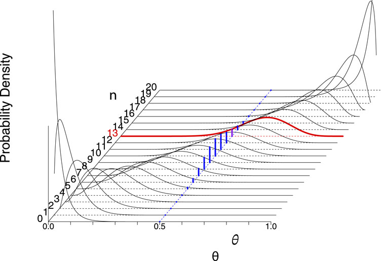
Figure 2. The relationship between the sampling distribution and likelihood functions for estimation of the success probability parameter,
Figure 3 shows a complementary case, where both the sample space and the parameter space are continuous, and the sample space is two-dimensional. It depicts the relationship between the sampling distributions for a model with a parameter
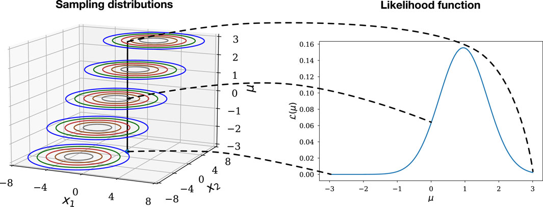
Figure 3. The relationship between the collection of sampling distributions comprising a parametric model for 2-dimensional continuous data (left) and the likelihood function (right).
For each choice of
The likelihood function quantifies how well each of the candidate sampling distributions—labeled by the parameter
If we need a word to characterise this relative property of different values of
Alas, colloquially “probability” and “likelihood” are synonyms, inviting misuse. The clash between the terminology and colloquial use is unfortunate; “predictive” or “prognostic” might have been better names for this function.
Fisher goes on:
Likelihood also differs from probability in that it is a differential element, and is incapable of being integrated: it is assigned to a particular point of the range of variation, not to a particular element [interval] (Fisher (1922), emphasis added).
He used stronger language earlier: “…the integration with respect to
The posterior PDF is closely related to the likelihood function, obtained simply by multiplying by a prior PDF and normalizing:
The posterior PDF is a probability distribution over
6 Priors are not (merely) penalties
The distinction between likelihood and probability points to the dual role of prior probabilities in Bayesian inference. Bayesian tutorials typically focus on priors as adjusters of the likelihood to account for base rates, parameter constraints (such as positivity), or results from prior experiments. This is indeed an important capability. But more fundamentally, the role of the prior is to “flip the conditional,” that is, to get us from likelihood to probability. With a probability distribution in hand, we are then able to use the LTP to address a myriad of questions involving consideration of composite hypotheses. In this section we elaborate on the role of priors in Bayesian inference, beyond the usually emphasized role of “modulating” the likelihood to account for prior information.
6.1 Intensive vs extensive quantities in inference
For an audience of physical scientists, a thermodynamic analogy may be illuminating. In thermodynamics, temperature is an intensive quantity. It is meaningful to talk about the temperature,
where
Priors play a similar role in Bayesian inference, not just modulating the likelihood function, but, more fundamentally, converting intensive likelihood to extensive probability. In thermodynamics, a region with a high temperature may have a small amount of heat if its volume is small, or if, despite having a large volume,
6.2 Typical vs optimal parameter values
Frequentist statistics includes penalized maximum likelihood methods that multiply the likelihood by a penalty function,
The penalty function shifts the location of the maximum. It looks like a prior, in that it multiplies the likelihood function, but because Bayesian calculations integrate rather than maximize over parameter space, the prior can do much more than shift the location of the mode (the location of the peak of the posterior) with respect to the maximum likelihood location.
A number of concepts from different areas of mathematics can help us understand the consequences of having a (summable/integrable) measure and not just a preference ordering over a parameter space:
We will give a sense of how these notions can help us understand the impact of integrating vs optimizing with two simple examples.
Consider
This phenomenon is not unique to discrete spaces. Consider now curve fitting with
The left panel of Figure 4 shows this quantitatively for
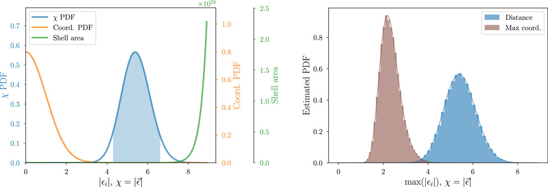
Figure 4. Elucidation of the nature of the typical set for a 30-dimensional standard normal distribution with coordinates
The lesson of these examples is that for high-dimensional spaces, the mode of a distribution is likely to be very atypical, in the sense that random draws from the distribution are unlikely to resemble the mode (in terms of the values of the PMF or PDF for the draws). These examples looked at properties of familiar sampling distributions, but the math does not care if we call a variable “data” or “parameter”—the notion of typical sets applies to distributions over large parameter spaces as well as to distributions over large sample spaces.
6.3 Example: histogram-based density estimation
As an example of these ideas at work in a parameter estimation setting, consider estimating a PDF for some continuous observable quantity via histogram data—say, galaxy fluxes grouped into a few dozen flux bins (a “number-counts” or “
where
For a Bayesian analysis, a tempting choice of prior, intending to be uninformative about the
Figure 5 tries to build insight into this question by looking at random samples from the prior. The left panel shows a stack of 10 random
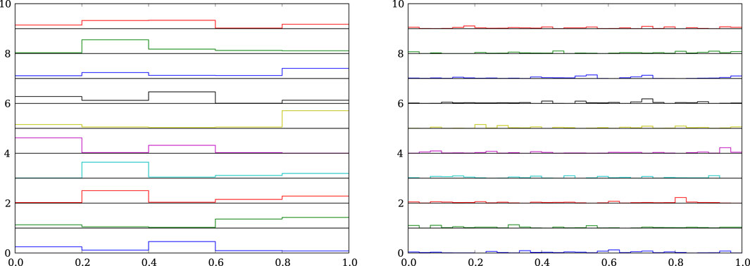
Figure 5. 10 samples of
A bit of analytical work confirms the visual impression (see Frigyik et al., 2010 for a tutorial covering the math). We can compute the marginal PDF for a particular
How might we fix this? Consider the family of symmetric Dirichlet priors, of the form
(the
How to set
Figure 6 shows samples from an aggregation-consistent prior with
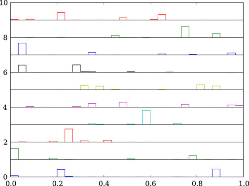
Figure 6. As in Figure 5, but with samples drawn from an aggregation-consistent symmetric Dirichlet distribution for
We have focused on the prior; what is the impact on the posterior? For estimating all
A lesson of this section is that we should be cautious and skeptical of our intuition when attempting inference in high-dimensional parameter spaces (Genovese et al. (2004) have urged similar caution from a frequentist perspective). Prior probabilities let us get something integrable from likelihood functions, enabling diverse useful calculations when we are interested in composite hypotheses. But the “extensive” (summable) nature of prior and posterior distributions means that parameter space volume effects can have surprising impacts on inference. If we think of priors merely as modulating or penalizing the likelihood function, it would seem that a uniform prior would not divert attention from the peak of the likelihood function. But the notion of typical sets, and the behavior of uniform priors in multinomial inference, alert us that even flat priors may divert attention from the maximum likelihood region when the parameter space is high-dimensional. On the one hand, this is a warning that optimization can be misleading; it can focus attention on parts of parameter space that are very atypical. On the other hand, it is also a warning against relying on low-dimension intuition, like equating prior uniformity with being noncommittal or uninformative. A practical lesson is to always look at samples from the prior, particularly when working in high-dimensional parameter spaces.
7 Nuisance parameters: marginalization vs optimization
Of the many tasks using the LTP listed in SS 4, one of the most important is marginalizing over nuisance parameters. It is very common (in our experience, essentially ubiquitous) for a data modeling problem to require introducing parameters that are not of direct scientific interest, but that are necessary for describing how the data relate to the quantities of interest. Estimation of the interesting quantities has to somehow account for the uncertainty in the uninteresting “nuisance” quantities. In this section we elaborate on how marginalization over nuisance parameters accomplishes this, in particular the role of parameter space volume in the behavior of marginal posterior PDFs.
A frequently-arising nuisance parameter setting is analysis of measurements contaminated by uncertain backgrounds or foregrounds. A somewhat more subtle but also prevalent setting is estimating population distributions (density estimation) or correlations and scaling laws for a population (regression), when the properties of members of the population are measured with uncertainty—so-called measurement error problems (statisticians use this term for density estimation with noisy measurements, or regression with noise in both the measured predictors/covariates (
In a Bayesian treatment of such measurement error problems (and in many frequentist formulations), the unknown true properties for each object formally appear as latent parameters, estimated with uncertainty. For inference about a population as a whole, the latent parameters are nuisance parameters, and their uncertainty must be propagated into population inferences. Importantly, in measurement error problems the number of latent parameters grows with sample size; as a result, even small inaccuracies in accounting for measurement error per-object can accumulate and lead to incorrect population-level inferences (Loredo, 2004). Hierarchical Bayesian (HB) models handle measurement error by marginalizing over the latent parameters. Some entry points into the rapidly growing literature on HB demographic modeling in astronomy include: Loredo (2004); Kelly (2012); Mandel (2012); Loredo (2013); Andreon and Hurn (2013); Hsu et al. (2018); Loredo and Hendry (2019); Mandel et al. (2019); Vitale (2020).
7.1 Understanding marginalization
Given the prevalence and importance of nuisance parameter problems in astronomy, it is worth building insight into how marginalization accounts for nuisance parameter uncertainty. To do so, we will consider the signal-plus-background setting, with interesting signal parameter,

Figure 7. Left: An example joint likelihood function for
Specifying the value of one parameter in a multiparameter problem is a composite hypothesis: specifying just
To summarize implications for
where the second line uses the numerator of BT, with likelihood function
Now factor that joint prior as the prior for
Since the marginalization integral is over
where we have defined the marginal likelihood function for
(where we suppress
To build insight into what marginalization accomplishes, we approximate the integral over
1. Assume the data are informative, so the prior PDF for
2. Approximate the remaining integral of
We need some notation to implement these steps. Let
Graphically,
The integral over
The first factor is the joint likelihood function maximized over
It corresponds to looking at the 3D
Assembling these results, we have this helpful approximation for the marginal likelihood function for
The last two factors are the data-dependent factors. Much of the work done by marginalization is captured in the profile likelihood factor. A naive approach to handling a nuisance parameter would be to fix it at its best-fit value. This would correspond to slicing
Figure 7 depicts a joint likelihood function that is a bivariate Gaussian function. Recall that a bivariate Gaussian may be written as the product of a Gaussian for one variable (say,
Figure 8 shows two scenarios where marginal and profile likelihood functions may noticeably differ (here
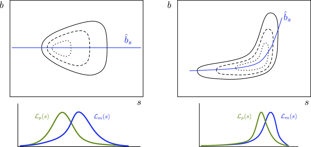
Figure 8. Illustration of two-parameter likelihood function geometries where marginalization and profile likelihood may lead to significantly different inferences. Top panels show joint likelihood functions for parameter of interest
7.2 Measurement error problems—handling many nuisance parameters
It is often the case that the nuisance parameter volume correction is noticeable in a single measurement, but not hugely significant; it may shift the profile likelihood function by only a fraction of its width. But the effect tends to be in a similar direction for similar measurements. When combining information across many measurements, the systematic effect from the nuisance parameter volume factor can accumulate, and ignoring it can corrupt aggregated inferences, such as demographic inferences.
Figure 9 illustrates this with a somewhat contrived but illuminating example7. For each of a set of
From a single pair of measurements, there is substantial uncertainty in both
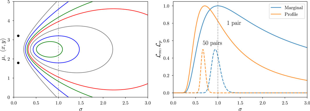
Figure 9. Joint, marginal, and profile likelihood functions for the normal pairs (Neyman-Scott) problem. Left: Joint likelihood function for the standard deviation
We should be able to improve inference by pooling information across many pairs of measurements. Each pair brings in more information about
The dashed curves in the right panel of Figure 9 show what happens when we accumulate information across multiple paired measurements (here drawn from a broad, uniform distribution, though the findings described here do not depend on this choice). Formally, we do this by computing a likelihood function for the full dataset that is the product of the likelihood functions for the pairs,
where
To make the point that such problems are not uncommon in astronomy, Figure 10 shows likelihood functions from simulated data for isolated dim point sources observed with a CCD camera with a critically-sampled Gaussian PSF (the calculations are based on the description of the Hyper Suprime-Cam pipeline in Bosch et al., 2018). The left panel is for a
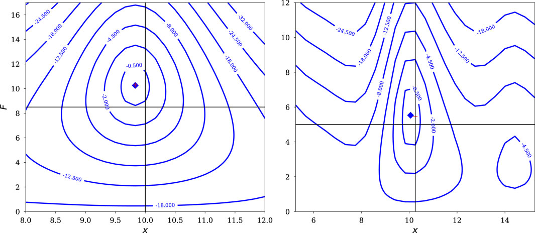
Figure 10. Likelihood functions as a function of flux,
For those requiring a frequentist solution to measurement error problems, there is a large and growing literature presenting numerous techniques specialized to specific problem settings. From a Bayesian perspective, specialized inference techniques are unnecessary; marginalization over latent parameters handles such problems generally and flexibly (though the resulting computational challenges can demand nontrivial computational algorithms specialized to different settings). Notably, even statisticians who generally favor frequentist methods recommend Bayesian approaches that marginalize over latent parameters in complicated settings, particularly for nonlinear modeling of data with heteroscedastic measurement error (i.e., with measurements that have differing standard deviations); see Carroll et al. (2006). Astronomical data commonly has heteroscedastic measurement error, and the ability of marginalization to flexibly accommodate this complication has been a strong motivation for the spread of Bayesian methods for measurement error problems in astronomy.
8 Systematic error and model misspecification
A well-known aphorism attributed to George Box motivates our final marginalization application area: “All models are wrong, but some are useful” (Box and Draper, 1987; see also Box, 1976). In some data analysis settings, we may be largely secure about our model, but still want to explore the possibility that inference may be corrupted by potential influences omitted from the model. In other settings we may knowingly adopt an approximate model, and want to account for the lack of fidelity to the data when we make inferences about salient features of the model. Here we briefly describe the role composite hypotheses and marginalization can play to improve uncertainty quantification in such settings. We consider two settings: first, where systematic error arises due to model selection uncertainty (i.e., whether to include terms for anticipated corrupting effects), and second, where a model aims to account only for salient features of a phenomenon, and we want to account for uncertainty in deliberately unmodeled details.
8.1 Systematic error and model selection uncertainty
A fairly common way astronomers try to account for systematic error from identified potential corrupting effects is to use a classical null hypothesis significance test (NHST) to see if there is significant evidence in the data for the effects. A statistic is devised to test for the presence of a potential effect; if the null hypothesis of no effect is not rejected, analysis proceeds assuming no effect is present. A significant issue with this approach is that failure to reject a null hypotheses need not correspond to a strong preference for the null over the alternative (see, e.g., Berger, 2003; Wasserstein and Lazar, 2016; Greenland et al., 2016; Wasserstein et al., 2019). Ideally we would like to take into account potential systematic effects, weighted in a way that measures the strength of evidence for or against their presence.
Marginal likelihoods can provide such a weighting (see the brief description of model averaging above). However, marginal likelihoods typically are more sensitive to the choice of prior than are parameter estimates—in particular, to the ranges of the parameter spaces considered for rival models—and one must be cautious about using them to account for systematic error.
An example of systematic error quantification using marginal likelihoods and Bayes factors is the work of Drell et al. (2000) (DLW00) exploring the potential impact of systematic error from source evolution on early analyses of the evidence for dark energy from measurements of Type Ia supernova (SN Ia) light curves (“SN cosmology”). The dark energy discovery papers found no significant evidence for SN Ia source evolution (dependence of light curve properties on redshift), and so assumed there was exactly zero evolution in their analyses. DLW00 computed Bayes factors indicating the data were equivocal regarding the presence of evolution. An important aspect of the calculation was consideration of a variety of priors for parameters in evolution models, to ensure the findings were robust. Allowing for plausibly small levels of evolution, and marginalizing over its impact, significantly weakened the strength of the evidence for dark energy, unless one assumed a flat cosmology, which was not justified at the time. Fortunately, within a few years accumulating evidence from other cosmological phenomena honed in on flat cosmologies. From the perspective of the DLW00 systematic error analysis, it was only in the context of this later evidence that the discovery of dark energy became secure.
8.2 Systematic error, overdispersion, and model discrepancy
In astronomy we often knowingly use models that capture only the salient features of a phenomenon. This is particularly true when first exploring a frontier area, where learning such features can provide significant insight, even if the salient feature model overlooks details. Examples include counting pulses in gamma-ray burst prompt light curves (where we may care only about the number of pulses and their time scales, not every minor wiggle), or modeling luminosity functions with broken power laws (where we would like to estimate a power law slope and a break luminosity, irrespective of minor bumps in the distribution). Simply adopting the salient feature model and ignoring model misspecification can corrupt inferences, in particular by providing artificially tight constraints on the salient model parameters.
One approach to handling this is to simply inflate sampling distributions. For example, in the statistics literature analyzing count data, it is common to adopt negative binomial (NB) rather than Poisson distributions at the outset, since the NB distribution has an extra parameter that can be used to overdisperse the predictive distribution for counts, and it includes the Poisson distribution as a special case (see, e.g., Hilbe 2011; de Souza et al. (2015) for an application in astronomy; see the Supplementary Appendix for a brief discussion of the NB distribution and its use for modeling overdispersion). Bonamente (2023) has adapted this idea to account for systematic error in astronomical data analysis of Poisson data in the regime where
We are developing complementary methods for salient feature modeling of Poisson count and point process data that are closely tied to use of NB distributions. But we do not adopt overdispersed distributions outright. In contrast to most applications of the Poisson distribution in the statistics literature, in many astrophysical applications there is a strong physical basis for adopting a Poisson distribution as the description of the repeated-sampling variability expected in the data—the so-called aleatoric uncertainty (from the Latin aleator for “dice player”). We use overdispersion to reflect a combination of aleatoric and epistemic sources of uncertainty (with the epistemic component capturing the systematic errors that may not vary randomly across replications).
We construct overdispersed distributions via representations that tie them to the underlying aleatoric sampling distribution via a plausible discrepancy mechanism (adapting the notion of additive discrepancy functions from Gaussian process emulation of computer models; see the Supplementary Appendix). We consider the actual intensity function (event rate) for the Poisson process governing the data to be the product of the parametric salient model rate that we wish to estimate, and a nonnegative discrepancy factor. Figure 11 illustrates the construction for a model for photon counts from a time-varying source, binned in time, used to estimate parameters of a salient light curve model. The blue histogram depicts the predictions of a Poisson model for the photon counts in bins, as expectation values,
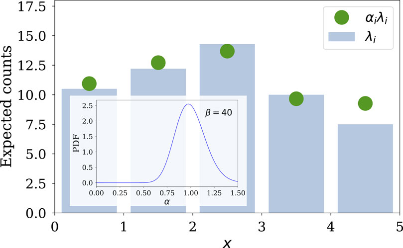
Figure 11. Depiction of the multiplicative discrepancy approach. Blue histogram shows the Poisson distribution PMF from a salient feature model. Green dots depict the PMF resulting from multiplying the Poisson expectation values by draws from a gamma distribution discrepancy process. Inset shows the unit-mean gamma distribution for the discrepancy factors.
The choice of a gamma distribution enables analytic marginalization over the discrepancy factors, producing a predictive PMF for the counts that is NB, with a variance that may be inflated with respect to that of a Poisson distribution. (See the Supplementary Appendix for further details.) More deeply, the gamma choice lets us introduce discrepancy in a manner that preserves aggregation consistency in a sense analogous to what we described above regarding Dirichlet priors for histograms. This framework explicitly acknowledges that the actual count variability distribution is expected to be Poisson. It also points toward generalizations that can apply to point data, and that can account for bin-to-bin correlations in the discrepancy. Details for specific astrophysical applications will be reported elsewhere.
9 More than Bayes’s theorem
The theme of this tutorial has been that BT and the LTP are partners in Bayesian inference—arguably unequal partners, with the LTP carrying much of the burden in analysis and computation. This is because of how common composite hypotheses are in astrophysical data analysis. We hope we have made a strong case that the role of the LTP and marginalization should be highlighted more prominently in the Bayesian astrostatistics literature, particularly in pedagogical presentations.
Python and R code producing figures from this paper are available at https://github.com/tloredo/MoreThanBT2024-Figures.
Data availability statement
The datasets presented in this article are not readily available because only small simulated datasets were used, for didactic purposes. Requests to access the datasets should be directed to bG9yZWRvQGFzdHJvLmNvcm5lbGwuZWR1.
Author contributions
TL: Conceptualization, Methodology, Writing–original draft, Writing–review and editing. RW: Conceptualization, Methodology, Writing–review and editing.
Funding
The author(s) declare financial support was received for the research, authorship, and/or publication of this article. This material is based upon work supported by the National Science Foundation under Grants No. DMS-2015386 and AST-2206339 (for TL), and DMS-2015382 (for RW).
Acknowledgments
We gratefully acknowledge the organizers and participants of the
Conflict of interest
The authors declare that the research was conducted in the absence of any commercial or financial relationships that could be construed as a potential conflict of interest.
Publisher’s note
All claims expressed in this article are solely those of the authors and do not necessarily represent those of their affiliated organizations, or those of the publisher, the editors and the reviewers. Any product that may be evaluated in this article, or claim that may be made by its manufacturer, is not guaranteed or endorsed by the publisher.
Supplementary material
The Supplementary Material for this article can be found online at: https://www.frontiersin.org/articles/10.3389/fspas.2024.1326926/full#supplementary-material
Footnotes
1John Tukey—best known for his work on the fast Fourier transform and exploratory data analysis—observed: “No body of data tells us all we need to know about its own analysis” (Tukey, 1977). Data do not “speak for themselves” in scientific arguments; data analysis considers the implications of data within some context. In this sense, data analysis (Bayesian or frequentist) is necessarily subjective and provisional, and a virtue of the Jeffreys/Cox/Jaynes notation is its recognition that all probabilities are conditional, at least depending on the context,
2In settings where the alternatives are labeled by a continuous parameter,
3A statement
4This idea is notoriously difficult to define rigorously; arguably there is not yet a sound definition. For an exceptionally accessible overview of the difficulties see Diaconis and Skyrms (2018).
5Readers new to model comparison should note that in the astronomy literature and some machine learning literature it is popular to use the term evidence for the marginal likelihood. (Bayesian evidence also appears, awkwardly implying there are Bayesian vs non-Bayesian forms of evidence.) We eschew this terminology. The data (and possibly additional contextual information) comprise the evidence, and in the Bayesian philosophy of science literature it has long been common to use
6The values of marginal likelihoods depend more sensitively on properties of prior distributions than do posterior PDFs for parameters; in particular, they are roughly inversely proportional to the prior ranges of parameters. As a result, formal Bayesian model comparison and model averaging are best reserved for problems where the analyst can strongly motivate priors (especially prior ranges), or quantitatively study how results depend on properties of priors. Good entry points to the literature on this (in both astronomy and statistics) include: Volinsky et al. (1999); Clyde and George (2004); Clyde et al. (2007); Trotta (2012). For a Bayesian perspective on model selection relying on measures of anticipated out-of-sample predictive performance (vs a priori prediction of the observed sample, as measured by marginal likelihood), see Gelman et al. (2014b).
7Statisticians know this problem as the Neyman-Scott problem, a well-known counterexample to maximum likelihood estimation (Neyman and Scott, 1948). Neyman and Scott did important work on statistics in astronomy. Although the Neyman-Scott problem was first described in an econometrics journal, they posed it in terms of measuring “some physical constant such as the radial velocity of a star or the velocity of light.” They noted the connection to measurement error problems, and described several settings in astronomy where the issues they addressed potentially arise. Our discussion here expands on a shorter treatment in Loredo (2004).
References
Andreon, S., and Hurn, M. (2013). Measurement errors and scaling relations in astrophysics: a review. Stat. Analysis Data Min. ASA Data Sci. J. 9 (1), 15–33. doi:10.1002/sam.11173
Berger, J. O. (2003). Could Fisher, Jeffreys and neyman have agreed on testing? Stat. Sci. 18, 1–32. doi:10.1214/ss/1056397485
Berger, J. O., and Berry, D. A. (1988). Statistical analysis and the illusion of objectivity. Am. Sci. 76, 159–165.
Berger, J. O., Liseo, B., and Wolpert, R. L. (1999). Integrated likelihood methods for eliminating nuisance parameters. Stat. Sci. 14, 1–28. doi:10.1214/ss/1009211804
Berger, J. O., and Wolpert, R. L. (1988). The likelihood principle. No. 6 in IMS lecture notes monogr. Ser. (SPIE). doi:10.1214/lnms/1215466210
Betancourt, M. (2017). A conceptual introduction to Hamiltonian Monte Carlo. arXiv:1701.02434 [stat] ArXiv: 1701.02434.
Bonamente, M. (2023). Systematic errors in the maximum-likelihood regression of Poisson count data: introducing the overdispersed X2 distribution. Mon. Notices R. Astronomical Soc. 522, 1987–2001. doi:10.1093/mnras/stad463
Bosch, J., Armstrong, R., Bickerton, S., Furusawa, H., Ikeda, H., Koike, M., et al. (2018). The Hyper Suprime-Cam software pipeline. Publ. Astronomical Soc. Jpn. 70, S5. doi:10.1093/pasj/psx080
Box, G. E. P. (1976). Science and statistics. J. Am. Stat. Assoc. 71, 791–799. doi:10.1080/01621459.1976.10480949
Box, G. E. P. (1980). Sampling and Bayes’ inference in scientific modelling and robustness. J. R. Stat. Soc. Ser. A General. 143, 383–430. Publisher: [Royal Statistical Society, Wiley]. doi:10.2307/2982063
Box, G. E. P., and Draper, N. R. (1987) “Empirical model-building and response surfaces,” in Wiley series in probability and mathematical statistics. New York: Wiley.
Carroll, R. J., Ruppert, D., Stefanski, L. A., and Crainiceanu, C. M. (2006) “Measurement error in nonlinear models: a modern perspective, vol. 105 of Monographs on Statistics and Applied Probability,”. second edn. Boca Raton, FL: Chapman and Hall/CRC. Available at: https://www.routledge.com/Measurement-Error-in-Nonlinear-Models-A-Modern-Perspective-Second-Edition/Carroll-Ruppert-Stefanski-Crainiceanu/p/book/9781584886334.doi:10.1201/9781420010138
Clyde, M., and George, E. I. (2004). Model uncertainty. Inst. Math. Statistics 19, 81–94. doi:10.1214/088342304000000035
Clyde, M. A., Berger, J. O., Bullard, F., Ford, E. B., Jefferys, W. H., Luo, R., et al. (2007). “Current challenges in bayesian model choice,”. Statistical challenges in modern astronomy IV. Editors G. J. Babu, and E. D. Feigelson, 371, 224.
Cover, T. M., and Thomas, J. A. (2006). Elements of information theory. 2nd ed edn. Hoboken, N.J.: Wiley-Interscience. doi:10.1002/047174882X
Cox, R. T. (1946). Probability, frequency and reasonable expectation. Am. J. Phys. 14, 1–13. doi:10.1119/1.1990764
de Souza, R. S., Hilbe, J. M., Buelens, B., Riggs, J. D., Cameron, E., Ishida, E. E. O., et al. (2015). The overlooked potential of generalized linear models in astronomy - III. Bayesian negative binomial regression and globular cluster populations. Mon. Notices R. Astronomical Soc. 453, 1928–1940. doi:10.1093/mnras/stv1825
Diaconis, P., and Skyrms, B. (2018). Ten great ideas about chance. Princeton: Princeton University Press. OCLC: ocn983825018.
Downey, A. B. (2021). Think Bayes: bayesian statistics in Python. second edition edn. Beijing Boston Farnham Sebastopol Tokyo: O’Reilly.
Drell, P. S., Loredo, T. J., and Wasserman, I. (2000). Type IA supernovae, evolution, and the cosmological constant. Astrophysical J. 530, 593–617. doi:10.1086/308393
Eadie, G. M., Speagle, J. S., Cisewski-Kehe, J., Foreman-Mackey, D., Huppenkothen, D., Jones, D. E., et al. (2023). Practical guidance for bayesian inference in astronomy. ArXiv:2302.04703. [astro-ph, stat]. doi:10.48550/arXiv.2302.04703
Fisher, R. A. (1912). On an absolute criterion for fitting frequency curves. Messenger Mathmatics 41, 155–160. doi:10.1214/ss/1029963260
Fisher, R. A. (1922). On the mathematical foundations of theoretical statistics. Philosophical Trans. R. Soc. Lond. Ser. A, Contain. Pap. a Math. or Phys. Character 222, 309–368. Publisher: The Royal Society. doi:10.1098/rsta.1922.0009
Frigyik, B. A., Kapila, A., and Gupta, M. R. (2010) “Introduction to the dirichlet distribution and related processes,” in Tech. Rep. UWEETR-2010-0006. Seattle, WA: University of Washington.
Gelman, A., Carlin, J. B., Stern, H. S., Dunson, D. B., Vehtari, A., and Rubin, D. B. (2014a) “Bayesian data analysis,” in Chapman and Hall/CRC texts in statistical science. third edition edn. Boca Raton: CRC Press.
Gelman, A., and Hennig, C. (2017). Beyond subjective and objective in statistics. J. R. Stat. Soc. Ser. A Statistics Soc. 180, 967–1033. doi:10.1111/rssa.12276
Gelman, A., Hwang, J., and Vehtari, A. (2014b). Understanding predictive information criteria for Bayesian models. Statistics Comput. 24, 997–1016. doi:10.1007/s11222-013-9416-2
Genovese, C. R., Miller, C. J., Michol, R. C., Arjunwadkar, M., and Wasserman, L. (2004). Nonparametric inference for the cosmic microwave background. Stat. Sci. 19, 308–321. doi:10.1214/088342304000000161
Good, I. J. (1950). Probability and the weighing of evidence. London: Charles Griffin and Co.). Google-Books-ID: k9g0AAAAMAAJ.
Good, I. J. (1985). Weight of evidence: a brief survey. In Bayesian statistics 2, eds. J. M. Bernardo, M. H. DeGroot, D. V. Lindley, and A. F. M. Smith (Amsterdam: Elsevier Science Publishers). 249–269.
Greenland, S., Senn, S. J., Rothman, K. J., Carlin, J. B., Poole, C., Goodman, S. N., et al. (2016). Statistical tests, P values, confidence intervals, and power: a guide to misinterpretations. Eur. J. Epidemiol. 31, 337–350. doi:10.1007/s10654-016-0149-3
Hilbe, J. M. (2011) “Negative binomial regression,”. Cambridge University Press. doi:10.1017/CBO9780511973420
Hsu, D. C., Ford, E. B., Ragozzine, D., and Morehead, R. C. (2018). Improving the accuracy of planet occurrence rates from kepler using approximate bayesian computation. Astronomical J. 155, 205. doi:10.3847/1538-3881/aab9a8
Jaynes, E. T. (2003). Probability theory: the logic of science. Cambridge University Press, 1. doi:10.1017/CBO9780511790423
Jeffreys, H. (1961). Theory of probability. Oxford classic texts in the physical sciences (Clarendon Press ; Oxford University Press), 3rd ed edn.
Kelly, B. C. (2012). “Measurement error models in astronomy,” in Statistical challenges. Lecture notes in statistics. Editors V. Modern Astronomy, E. D. Feigelson, and G. J. Babu (Springer New York), 147–162.
Lindley, D. V. (2000). The philosophy of statistics. J. R. Stat. Soc. Ser. D (The Statistician) 49, 293–337. doi:10.1111/1467-9884.00238
Lindley, D. V., Barndorff-Nielsen, O., Elfving, G., Harsaae, E., Thorburn, D., Hald, A., et al. (1978). The bayesian approach [with discussion and reply]. Scandinavian Journal of Statistics 5, 1–26. Publisher: [Board of the Foundation of the Scandinavian Journal of Statistics, Wiley].
Loredo, T. J. (1992). The promise of bayesian inference for astrophysics. In Statistical challenges in modern astronomy, eds. E. D. Feigelson, and G. J. Babu (New York, NY: Springer). 275–297. doi:10.1007/978-1-4613-9290-3_31
Loredo, T. J. (1999). “Computational technology for bayesian inference,”. Astronomical data analysis software and systems VIII. Editors D. M. Mehringer, R. L. Plante, and D. A. Roberts, 172, 297.
Loredo, T. J. (2004). Accounting for source uncertainties in analyses of astronomical survey data. AIP Conference Proceedings (AIP Publishing) 735, 195–206. doi:10.1063/1.1835214
Loredo, T. J. (2012). “Rotating stars and revolving planets: bayesian exploration of the pulsating sky * - oxford scholarship,” in Bayesian statistics 9. Editors J. M. Bernardo, M. J. Bayarri, J. O. Berger, A. P. Dawid, D. Heckerman, A. F. M. Smithet al. (Valencia, Spain: Oxford University Press), 361–392. doi:10.1093/acprof:oso/9780199694587.003.0012
Loredo, T. J. (2013). “Bayesian astrostatistics: a backward look to the future,” in Astrostatistical challenges for the new astronomy. Editor J. M. Hilbe (Springer New York. Springer Series in Astrostatistics), 15–40. doi:10.1007/978-1-4614-3508-2_2
Loredo, T. J., and Hendry, M. A. (2019). Multilevel and hierarchical Bayesian modeling of cosmic populations. arXiv e-prints 1911, arXiv1911, 12337.
Mandel, I., Farr, W. M., and Gair, J. R. (2019). Extracting distribution parameters from multiple uncertain observations with selection biases. Monthly Notices of the Royal Astronomical Society 486, 1086–1093. doi:10.1093/mnras/stz896
Mandel, K. S. (2012). “Hierarchical bayesian models for type Ia supernova inference,”. Statistical Challenges in Modern Astronomy V. Editors E. D. Feigelson, and G. J. Babu (New York: Springer), 902, 209–218. Conference Name: Statistical Challenges in Modern Astronomy V ADS Bibcode: 2012LNS…902.209M. doi:10.1007/978-1-4614-3520-4_20
Marin, J.-M., and Robert, C. P. (2010). On resolving the Savage–Dickey paradox. Electronic Journal of Statistics 4, 643–654. doi:10.1214/10-EJS564
Neyman, J., and Scott, E. L. (1948). Consistent estimates based on partially consistent observations. Econometrica 16, 1–32. Publisher: [Wiley, Econometric Society]. doi:10.2307/1914288
Perks, W. (1947). Some observations on inverse probability including a new indifference rule. Journal of the Institute of Actuaries (1886-1994) 73, 285–334. doi:10.1017/s0020268100012270
Tak, H., Ghosh, S. K., and Ellis, J. A. (2018). How proper are Bayesian models in the astronomical literature? Monthly Notices of the Royal Astronomical Society 481, 277–285. doi:10.1093/mnras/sty2326
Trotta, R. (2012). Recent advances in cosmological bayesian model comparison. In Astrostatistics and data mining, eds. L. M. Sarro, L. Eyer, W. O’Mullane, and J. De Ridder (New York, NY: Springer). 3–15. doi:10.1007/978-1-4614-3323-1_1
Tukey, J. W. (1977) “Exploratory data analysis,” in Addison-Wesley series in behavioral science. Reading, Mass: Addison-Wesley Pub. Co.
Vardanyan, M., Trotta, R., and Silk, J. (2011). Applications of Bayesian model averaging to the curvature and size of the Universe. Monthly Notices of the Royal Astronomical Society 413, L91–L95. doi:10.1111/j.1745-3933.2011.01040.x
Vitale, S. (2020). One, No one, and one hundred thousand – inferring the properties of a population in presence of selection effects. arXiv2007.05579 [astro-ph, physicsgr-qc] ArXiv
Volinsky, C. T., Raftery, A. E., Madigan, D., and Hoeting, J. A. (1999). Bayesian model averaging: a tutorial (with comments by M. Clyde, David Draper and E. I. George, and a rejoinder by the authors). Statistical Science 14, 382–417. doi:10.1214/ss/1009212519
Wasserstein, R. L., and Lazar, N. A. (2016). The ASA statement on p-values: context, process, and purpose. The American Statistician 70, 129–133. 00–00doi. doi:10.1080/00031305.2016.1154108
Wasserstein, R. L., Schirm, A. L., and Lazar, N. A. (2019). Moving to a world beyond “p < 0.05”. The American Statistician 73, 1–19. doi:10.1080/00031305.2019.1583913
Wilson, A. G., and Izmailov, P. (2020). “Bayesian deep learning and a probabilistic perspective of generalization,”. Advances in neural information processing systems. Editors H. Larochelle, M. Ranzato, R. Hadsell, M. F. Balcan, and H. Lin (Curran Associates, Inc.), 33, 4697–4708.
Keywords: astrostatistics, bayesian methods, Poisson distribution, nuisanace parameters, systematic error, maximum likelihood, marginalization
Citation: Loredo TJ and Wolpert RL (2024) Bayesian inference: more than Bayes’s theorem. Front. Astron. Space Sci. 11:1326926. doi: 10.3389/fspas.2024.1326926
Received: 24 October 2023; Accepted: 18 June 2024;
Published: 22 October 2024.
Edited by:
Eric D. Feigelson, The Pennsylvania State University (PSU), United StatesReviewed by:
Ewan Cameron, Curtin University, AustraliaJohannes Buchner, Max Planck Institute for Extraterrestrial Physics, Germany
Copyright © 2024 Loredo and Wolpert. This is an open-access article distributed under the terms of the Creative Commons Attribution License (CC BY). The use, distribution or reproduction in other forums is permitted, provided the original author(s) and the copyright owner(s) are credited and that the original publication in this journal is cited, in accordance with accepted academic practice. No use, distribution or reproduction is permitted which does not comply with these terms.
*Correspondence: Thomas J. Loredo, bG9yZWRvQGFzdHJvLmNvcm5lbGwuZWR1
 Thomas J. Loredo
 Robert L. Wolpert