 Ming Wang
 Chihang Yang
 Yang Sun
 Hao Zhang
- 1University of Chinese Academy of Sciences, Beijing, China
- 2Key Laboratory of Space Utilization, Technology and Engineering Center for Space Utilization, Chinese Academy of Sciences, Beijing, China
- 3Xi'an Modern Control Technology Research Institute, Xi'an, China
Given the current enthusiasm for lunar exploration, the 2:1 resonant distant retrograde orbit (DRO) in Earth-Moon space is of interest. To gain an in-depth understanding of the complex dynamic environment in cislunar space and provide more options for parking orbits, this paper investigates the existence of quasi-periodic orbits near the 2:1 resonant DRO in the circular restricted three-body problem (CR3BP). Firstly, the numerical computation approach, continuation strategy, and stability analysis method of quasi-periodic orbits are introduced. Then, addressing the primary challenges in the continuation progress, we have developed an adaptive continuation algorithm with automatic adjustment of the step size and the number of discrete points that characterize the invariant torus. Finally, two types of 2D quasi-DROs and their linear stability properties are explored. Using Poincaré sections, we investigated the boundaries of the maximum extent attainable by both 2D quasi-DRO families in the CR3BP at a specific Jacobi energy, confirming that both types of quasi-periodic families have reached their respective boundaries. The algorithm described in this paper is beneficial for facilitating the computation of quasi-periodic families and aids in discovering additional potential dynamical structures.
1 Introduction
In recent years, there has been a resurgence of enthusiasm for lunar exploration, making cislunar space a focal point for human exploration and research. Several space missions, some successfully launched in the past years, and others scheduled for the near future, have been proposed for verification, scientific exploration, or space observation purposes. Notable missions include CAPSTONE (Gardner et al., 2023), KPLO (Song et al., 2021), ARTEMIS 1 (Williams et al., 2023), and VIPER (Colaprete et al., 2019). The exploration of cislunar space presents a prosperous prospect. As a stable orbit family suitable for long-term parking in cislunar space (Bezrouk and Parker, 2014), distant retrograde orbits (DROs) have garnered particular attention from institutions all over the world. The stability and strategic significance of DROs make them a compelling choice. According to existing literature, DROs have four primary applications: serving as a space harbor for scientific exploration, a candidate orbit for space domain awareness, a transit station for deep space exploration, and a relay orbit for inter-satellite links (Smitherman and Griffin, 2014; Stramacchia et al., 2016; Conte et al., 2018; Wang et al., 2019).
While scholars have extensively studied the dynamics and structural characteristics of DROs in the CR3BP, this knowledge falls short for practical engineering applications. For instance, the eclipse situation on DROs is suboptimal since DROs are nearly located on the Earth-Moon plane even when transitioned to the ephemeris model. This directly impacts the on-orbit stability of spacecraft. McCarthy B. P. and Howell (2021) have explored the potential for eclipse avoidance in quasi-DROs with
The CR3BP stands out as the simplest dynamic model for studying quasi-periodic motion in a multi-body system. In this model, the solution space is composed of four types of behaviors: equilibrium points, periodic orbits, quasi-periodic orbits, and chaotic motion (Folta et al., 2016). Olikara and Howell (2010) computed the family of Earth-Moon
The computation method of quasi-periodic orbits has undergone a transition from analytical or semi-analytical methods to full numerical methods, as discussed in Farquhar and Kamel (1973), Gómez et al. (1998), Jorba and Masdemont (1999), Hou et al. (2015). Analytical or semi-analytical methods like the Poincare-Lindstedt method and center manifold reduction often face challenges with small convergence regions. Therefore, we prefer the numerical method in this manuscript, specifically the GMOS (Gomez-Mondelo-Olikara-Scheeres) algorithm (Olikara and Scheeres, 2012), which iteratively computes the invariant curves represented by Fourier series on a stroboscopic map using Newton’s method. For additional details on other numerical methods, one can refer to Baresi et al. (2018) and the references therein. Numerous works in the literature have been dedicated to the calculation of quasi-periodic orbits or quasi-periodic families. Some focus on calculation skills, while others address computational efficiency (Schilder et al., 2005; Sánchez and Net, 2013; Olikara, 2016). Few studies address whether the continuation reaches the boundary, which demarcate the regions of bounded motion and chaos. As they do not clarify whether the failure of continuation is due to encountering resonance or reaching the continuation boundary, there is a high probability that the quasi-periodic families are incomplete. Nevertheless, it is crucial to recognize the boundaries of chaos and order.
Motivated by the above analyses, this paper delves into the quasi-periodic motion and its stability properties near the 2:1 resonant DRO in the CR3BP. However, The continuation process is not without challenges. Specifically, the quasi-periodic families encounter a series of resonant regions during the continuation process, requiring an increased number of sampling nodes to achieve a specified accuracy, as reported in Jorba and Olmedo (2009). If the step size is inappropriate, it can easily lead to singularities, resulting in program failure. Furthermore, the shape and size of the torus are factors determining the number of Fourier nodes, as discussed in Rosales et al. (2021). Considering these factors, we have developed an adaptive continuation framework that adjusts the continuation step size and the number of nodes to save computational time and enhance robustness. Pseudo-arclength continuation and natural parameter continuation schemes are employed for cross-verification. Additionally, with the aid of the Poincaré map and bifurcation theory, we have confirmed that the quasi-DRO families have reached their continuation boundaries.
The remaining structure of this paper is outlined as follows. Section 2 introduces the circular restricted three-body problem and presents a visual representation of the 2:1 resonant Distant Retrograde Orbit. Section 3 provides a detailed overview of the computational framework, discussing the challenges encountered in our calculations and introducing an adaptive algorithm. In Section 4, two types of 2D quasi-periodic orbit families are presented, and the boundaries of the orbit families are also verified. Stability analysis is conducted in Section 5. Lastly, conclusions are drawn in Section 6.
2 Preliminaries
2.1 Circular restricted three-body model
The circular restricted three-body problem (CR3BP) is a widely used model for studying spacecraft motion in multi-body systems. It describes the motion of an infinitesimal mass influenced by two massive bodies, such as the Earth and the Moon in cislunar space, within a rotating coordinate system centered at the Earth-Moon barycenter. The
In Equation 1,
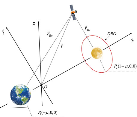
Figure 1. Diagram of the circular restricted three-body problem. The red curve represents the 2:1 DRO.
In Equation 2, the effective potential
In Equation 3,

Table 1. Relevant physical constants in the Earth-Moon system.
The CR3BP is an autonomous system with a unique energy integral, i.e., the Jacobi constant as displayed in Equation 4,
2.2 2:1 DRO in the CR3BP
The DROs are a special family of periodic orbits in the CR3BP, which moves clockwise (retrograde) around the Moon in cislunar space. Due to the symmetry of the DRO family about the
where
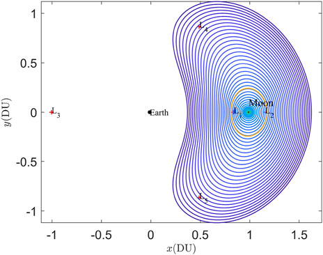
Figure 2. DRO family in the Earth-Moon system. The orange curve is the 2:1 resonant DRO.
In general, the resonant ratio
3 Computation method of quasi-periodic orbits
A typical approach to exploring the phase space of a dynamical system involves the investigation of its invariant sets. The term “invariant sets” encompasses equilibrium points, periodic orbits, and invariant tori within the system (Rosales et al., 2021). These invariant sets, along with their associated invariant manifolds, provide valuable insights into the evolution of dynamical systems within phase space. Generally, quasi-periodic motion occurs on two- or higher-dimensional invariant torus surfaces. Equilibrium points and periodic orbits can be considered as special instances of invariant tori—specifically, zero- and one-dimensional invariant tori within phase space (Olikara and Scheeres, 2012).
3.1 Initial guess of invariant tori
For Hamiltonian systems, the linear approximation of the quasi-periodic invariant torus is often related to the center manifolds of the periodic orbits (Lujan and Scheeres, 2022). Considering periodic orbits as one-dimensional invariant tori, there exists a differential isomorphic mapping
In Equation 6,
It should be noted that all frequencies are nonresonant in Equation 7, i.e., for any
3.2 Invariant constriant
Quasi-periodic motion occurs on an invariant torus in a specific manner. As mentioned earlier, for any point initially located on the surface of the torus, when it is integrated for a certain time, the final state is still on the torus but rotated by a fixed phase compared to the initial state. This property forms the basis for calculating invariant tori or quasi-periodic orbits. Since all phase components do not resonate with each other, the quasi-periodic orbit gradually fills the entire invariant torus as time evolves. Therefore, computing a quasi-periodic orbit is equivalent to computing an invariant torus. The computation algorithm used in this paper is based on the GMOS algorithm proposed by Olikara and Scheeres, as described in Olikara and Scheeres (2012). Pseudo-arclength continuation and natural parameter continuation are both explored for verification purposes.
For the dynamical system of interest, it can typically be expressed as an ordinary differential equation in state space form, as follows (Jorba and Olmedo, 2009):
where
where
therefore, from a numerical point of view, computation of quasi-periodic torus is equivalent to seeking the solution of Equation 10. A practical numerical method is to represent the high-dimensional reduced torus on the stroboscopic map in the form of (truncated) Fourier series,
where
The first phase angle component is typically fixed (usually set to 0), then for a (
In Equation 13, for each phase angle element
In Equation 14,
3.3 Continuation of invariant tori
The continuation process begins with the calculation of the first invariant torus. As is discussed at the beginning of this section, the initial guess is provided by linearizing the center manifold of the periodic orbit. Let
and the invariant constraint can be given as
It should be noted that the dimension of free variable
Before proceeding the continuation process, some additional phase angle constraints should also be added to ensure the desired direction of continuation. This is because for an invariant torus, any point on the torus satisfies the above constraint equations, namely,
In Equation 17, the partial derivatives
Equation 18 is derived through the total differential equation. By now, the augmented constraint matrix can be obtained as
Two major challenges during the computation process are the determination of sampling nodes and overcoming the resonant singularity. As mentioned in Rosales et al. (2021), the convergence of Newton’s method does not necessarily imply that the solution accurately represents the torus. Assume
In this manuscript, tol2 is referred to as the torus verification accuracy, while the convergence accuracy for Newton’s method is denoted as tol1. If Equation 19 is not satisfied, a higher-order Fourier series is added (with more samples accordingly), and then the differential correction is repeated. The number of sampling points is not fixed throughout the continuation process. Generally, the more complex, distorted, and larger the invariant torus, the more sampling points are required.
Since the quasi-periodic torus forms a Cantor set in the phase angle space, another challenge when resonance occurs is the singularity phenomenon as the continuation progresses. During singularity, the invariant torus becomes highly distorted, and nonlinearity sharply increases. A viable strategy is to dynamically adjust the step size within a specified range when singularity occurs until it crosses the resonant regions. Additionally, a hybrid pseudo-arclength continuation and natural parameter continuation are employed with various initial step sizes to enhance the reliability of results. The above analysis is summarized in Algorithm 1.
Algorithm 1.Adaptive continuation framework.
Require: The first converged invariant torus
Ensure: A definite quasi-periodic family
1: Let
2: Let
3:
4: Obtain the initial quasi-periodic orbit, and check its accuracy
5: while
6: Update the initial guess of
7: if
8: scale
9: if
10: stop
11: end if
12: continue
13: else
14:
15: end if
16: if
17:
18: if
19: turn to line 8
20: else
21: add
22: if
23: stop
24: end if
25: continue
26: end if
27: continue
28: else
29:
30: end if
31: save
32: end while
It should be noted that we introduce
3.4 Linear stability of invariant tori
The stability analysis of an invariant set can provide insight into the evolution of the manifold structure in phase space. The methods we adopt here are based on those described in Jorba, 2001. The first term of invariant constraint in Equation 10 has the differential form as follows:
Jorba shows that, in reducible case, the eigenstructure of matrix
The magnitude of the eigenvalues reflects the stability information. A convenient metric to measure the stability of invariant objects is the stability exponent, which is defined as:
If all the stability exponents
4 Quasi-periodic orbits in the CR3BP
4.1 The center manifolds of 2:1 DRO and resonance ratios near their phase angles
During the continuation process of quasi-periodic orbits, encountering resonance among the phase angles characterizing the torus is inevitable. Resonance phenomena often signify the presence of other periodic orbits in phase space. If resonance regions are not stepped over during the continuation process, quasi-periodic orbits will deviate from their initial continuation direction. Consequently, the torus will undergo distortion as the continuation progresses, leading to a significant increase in nonlinearity. In previous literatures, while resonance phenomena were acknowledged during the computation of quasi-periodic orbits, it failed to elucidate whether the failure in orbit continuation resulted from encountering strong resonance or if the orbit family reached the boundaries of continuation. Consequently, the computed orbit families in these studies are essentially incomplete. Considering these factors, in this section, we initially elaborate on the resonance ratios that quasi-periodic motion near the 2:1 DRO might encounter.
Figure 3 depicts the relationship between the phase angles of center manifolds and the Jacobi energy of the entire DRO family, where the phase angles of the center manifolds align with the phase angles of the eigenvalues
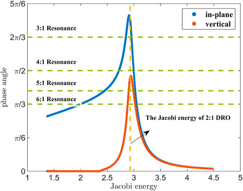
Figure 3. The relationship between the phase angles of center manifolds and the Jacobi energy of the entire DRO family.

Table 2. The center manifolds associated with the 2:1DRO in Earth-Moon system.
Douskos et al. (2007) investigated the impact of resonances on the in-plane stability region in the vinctiny of DROs. Their findings revealed that, with the exception of the period-tripling DRO (P3DRO), all resonant orbits bifurcating from the DROs are situated within the stable region and gradually approach the boundary of the stable region, namely, P3DRO. Hence, for the in-plane 2D quasi-DROs family around the 2:1 DRO, as the continuation progresses, the quasi-periodic family will be impeded by the resonance ratio 1/3, and the phase angle gradually decreases and eventually approaches
4.2 In-plane 2D quasi-DROs family
2D quasi-periodic orbits can be characterized by two phase angles. The first phase
Figure 4 depicts the relationship between the stroboscopic mapping period and the rotation angle
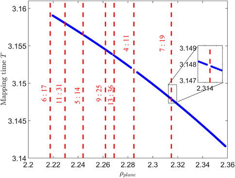
Figure 4. The relationship between the stroboscopic mapping period and the rotation angle ρin-plane of the plane 2D quasi-DRO family.
Figure 5 shows four in-plane 2D quasi-DROs with different rotation angles, where the red curves represent the invariant torus on the stroboscopic mapping defined at two vertically crossing points of 2:1 DRO, the yellow curve corresponds to the DRO orbit, and the blue region represents the densely covered area of the quasi-periodic orbits. It can be observed that the size of the invariant torus increases as the rotation angle
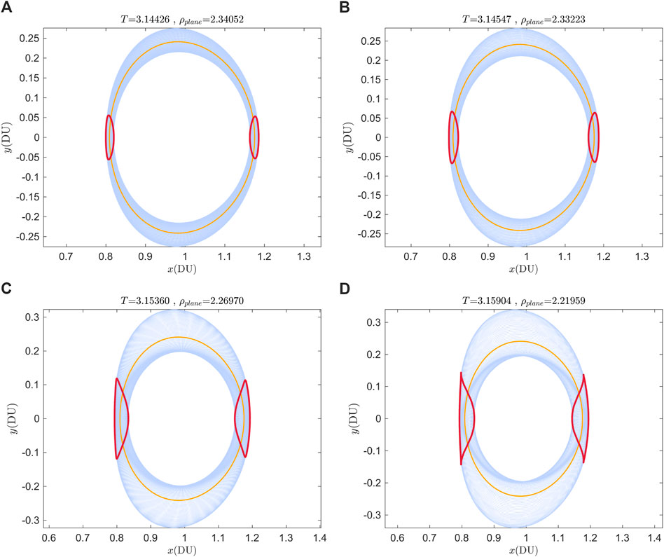
Figure 5. Four members of the in-plane 2D quasi-DROs family. (A) T = 3.14426, ρplane = 2.34052. (B) T = 3.14547, ρplane = 2.33223. (C) T = 3.15360, ρplane = 2.26970. (D) T = 3.14426, ρplane = 2.34052.
Record the intersections between the in-plane 2D quasi-DROs and the Poincaré section
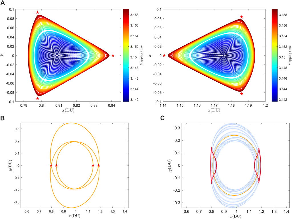
Figure 6. (A) The projection of the in-plane 2D quasi-DROs family on the Poincaré section, and the red pentagram represents the P3DROs. (B) the P3DROs with equal Jacobi energy as 2:1 DROs. (C) The twisted torus between the in-plane 2D quasi-DROs family and the P3DROs.
4.3 Vertical 2D quasi-DROs family
Figure 7 illustrates the relationship between the stroboscopic mapping time
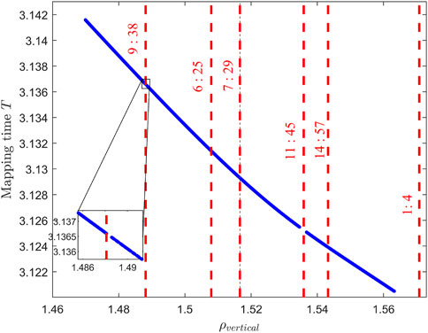
Figure 7. The relationship between the stroboscopic mapping period and the rotation angle ρvertical of the vertical 2D quasi-DROs family.
Figure 8 shows four quasi-periodic orbits at different rotation angles. As the continuation progresses, the size of the vertical quasi-periodic orbits in the
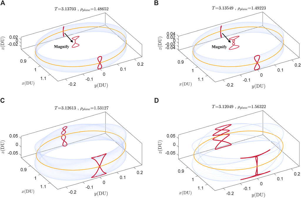
Figure 8. Four members of the vertical 2D quasi-DROs family. (A) T = 3.13703, ρvertical = 1.48652. (B) T = 3.13549, ρvertical = 1.49223. (C) T = 3.12613, ρvertical = 1.53127. (D) T = 3.12049, ρvertical = 1.56322.
The analysis process, utilizing the Poincaré section technique, for the vertical 2D quasi-DROs is the same as that for the in-plane 2D quasi-DROs. The difference lies in projecting the state variables
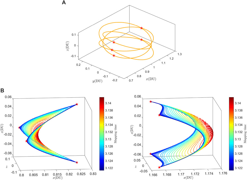
Figure 9. (A) The projection of the vertical 2D quasi-DROs family on the Poincaré section, and the red pentagram represents the P4DROs. (B) the P4DROs with equal Jacobi energy as 2:1 DROs.
Note that when the projections of the vertical 2D quasi-DROs and the P4DRO on the Poincaré section are positioned to the left of the Moon,
Figure 10 validates our previous conclusion that, when the Jacobi energy is 2.93052, P3DRO and P4DRO are the boundaries of the in-plane 2D quasi-DROs and vertical 2D quasi-DROs, respectively. It should be noted that P4DRO only serves as the boundary of the vertical 2D quasi-DROs when the Jacobi energy is colse to 2.93052. The phase angle of the vertical center manifold of DROs undergoes significant changes when the Jacobi energy is in the range of 2.8–3.2. Therefore, if the phase angle of the vertical center manifold of DRO approaches 1/5 or 1/6, the boundary of vertical 2D quasi-periodic orbits might be associated with other resonant DROs. However, this aspect is beyond the scope of this study.
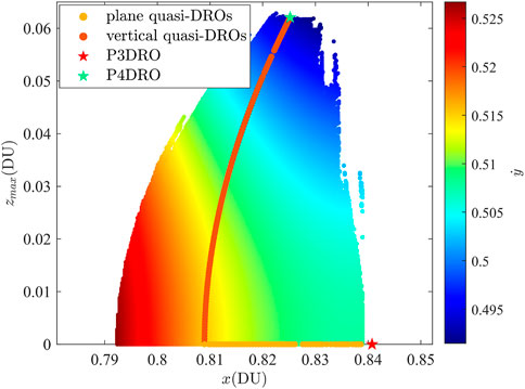
Figure 10. Characteristic parameter space of quasi-DROs at a Jacobi constant of 2.93052. Magenta and yellow scatters represent 2D vertical and in-plane quasi-periodic families, respectively. Red and green pentagram represent the P3DRO and P4DRO, respectively.
5 Stability analysis
The stability analysis of these two families is conducted in this section. For Hamiltonian systems with six-dimensional state space, the Floquent matrix of invariant objects is symplectic, leading to all eigenvalues appearing in the form of three recipocal pairs. Since the stroboscopic is autonomous in the CR3BP, all torus has a pair of eigenvalues equal to 1, and futher, equal to
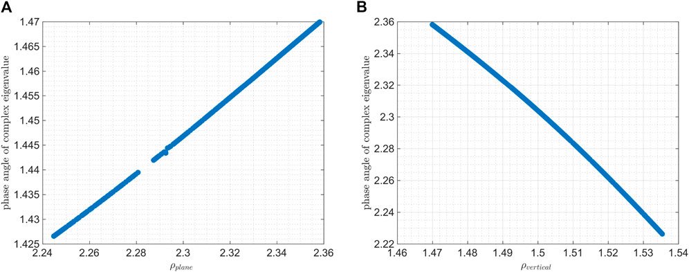
Figure 11. (A) Variation of the phase angles of the center manifolds for the in-plane 2D quasi-DROs with respect to
Therefore, both types of quasi-periodic orbits are long-term stable, offering more orbit choices for mission design.
6 Conclusion
In this paper, we have explored the dynamical structure near 2:1 resonant distant retrograde orbit in the circular restricted three-body problem. An adaptive continuation framework with adjustable step size and sampling nodes is proposed to solve the challenges encountered in the calculation of quasi-periodic families. The 2D plane and vertical quasi-periodic families are computed, respectively. Since the family of quasi-periodic orbits is Cantorian, a series of resonant regions will be encountered as the family evolves, leading to some “gaps” in the continuation process and the phenomenon of singularity of the invariant torus. In addition, we have observed that denser regions will occur in the coverage of quasi-periodic orbits when the rotation angle is close to resonance.
As a preliminary attempt, the geometric boundary that can be reached by the 2D quasi-periodic families in the CR3BP has been analyzed using the Poincaré map method. It has been verified by numerical simulation that the P3DRO and P4DRO are geometric boundaries of the 2D in-plane and vertical quasi-DROs. These dynamical structures greatly enrich the knowledge of the phase space near 2:1 resonant DRO, which is a major destination for cislunar space exploration.
As the CR3BP represents the most simplified model of multi-body dynamics, it disregards the eccentricity of the Moon’s orbit and the perturbative effects of the Sun. Future research will extend to examine the existence of quasi-periodic orbit families when these factors are incorporated. Additionally, future work will focus on applying these dynamical structures to space missions, including formation flying, transfer trajectories, and eclipse mitigation.
Data availability statement
The original contributions presented in the study are included in the article/supplementary material, further inquiries can be directed to the corresponding author.
Author contributions
MW: Writing–original draft, Writing–review and editing, Methodology, Validation, Conceptualization. CY: Methodology, Writing–review and editing. YS: Methodology, Writing–review and editing. HZ: Conceptualization, Funding acquisition, Methodology, Supervision, Validation, Writing–review and editing.
Funding
The author(s) declare that financial support was received for the research, authorship, and/or publication of this article. This work was supported by the Strategic Priority Research Program of the Chinese Academy of Sciences (Grant No. XDA30010200).
Conflict of interest
The authors declare that the research was conducted in the absence of any commercial or financial relationships that could be construed as a potential conflict of interest.
Publisher’s note
All claims expressed in this article are solely those of the authors and do not necessarily represent those of their affiliated organizations, or those of the publisher, the editors and the reviewers. Any product that may be evaluated in this article, or claim that may be made by its manufacturer, is not guaranteed or endorsed by the publisher.
Reference
Baresi, N., Olikara, Z. P., and Scheeres, D. J. (2018). Fully numerical methods for continuing families of quasi-periodic invariant tori in astrodynamics. J. astronautical Sci. 65, 157–182. doi:10.1007/s40295-017-0124-6
Bezrouk, C. J., and Parker, J. (2014). “Long duration stability of distant retrograde orbits,” in AIAA/AAS Astrodynamics Specialist Conference, San Diego, CA, August 4–7, 2014.4424
Colaprete, A., Andrews, D., Bluethmann, W., Elphic, R. C., Bussey, B., Trimble, J., et al. (2019). “An overview of the volatiles investigating polar exploration rover (viper) mission,” in AGU fall meeting abstracts, Bowie, MD, November 3–4, 2021.
Conte, D., Di Carlo, M., Ho, K., Spencer, D. B., and Vasile, M. (2018). Earth-mars transfers through moon distant retrograde orbits. Acta Astronaut. 143, 372–379. doi:10.1016/j.actaastro.2017.12.007
Douskos, C., Kalantonis, V., and Markellos, P. (2007). Effects of resonances on the stability of retrograde satellites. Astrophysics Space Sci. 310, 245–249. doi:10.1007/s10509-007-9508-6
Farquhar, R. W., and Kamel, A. A. (1973). Quasi-periodic orbits about the translunar libration point. Celest. Mech. 7, 458–473. doi:10.1007/bf01227511
Folta, D., Bosanac, N., Cox, A., and Howell, K. (2016). “The lunar icecube mission design: construction of feasible transfer trajectories with a constrained departure,” in AIAA Space Flight Mechanics Meeting, Napa, CA, February 14–18, 2016
Gardner, T., Cheetham, B., Parker, J., Forsman, A., Kayser, E., Thompson, M., et al. (2023). Capstone: a summary of a highly successful mission in the cislunar environment.
Gómez, G., Masdemont, J., and Simó, C. (1998). Quasihalo orbits associated with libration points. J. Astronautical Sci. 46, 135–176. doi:10.1007/bf03546241
Hou, X., and Liu, L. (2011). On quasi-periodic motions around the collinear libration points in the real earth–moon system. Celest. Mech. Dyn. Astronomy 110, 71–98. doi:10.1007/s10569-011-9340-8
Hou, X. Y., and Liu, L. (2010). On quasi-periodic motions around the triangular libration points of the real earth–moon system. Celest. Mech. Dyn. Astronomy 108, 301–313. doi:10.1007/s10569-010-9305-3
Hou, X. Y., Xin, X., Scheeres, D. J., and Wang, J. (2015). Stable motions around triangular libration points in the real earth–moon system. Mon. Not. R. Astron Soc. 454, 4172–4181. doi:10.1093/mnras/stv2216
Jorba, A. (2001). Numerical computation of the normal behaviour of invariant curves of n-dimensional maps. Nonlinearity 14, 943–976. doi:10.1088/0951-7715/14/5/303
Jorba, À., Jorba-Cuscó, M., and Rosales, J. J. (2020). The vicinity of the earth–moon l1 point in the bicircular problem. Celest. Mech. Dyn. Astronomy 132, 11. doi:10.1007/s10569-019-9940-2
Jorba, A., and Masdemont, J. (1999). Dynamics in the center manifold of the collinear points of the restricted three body problem. Phys. D. Nonlinear Phenom. 132, 189–213. doi:10.1016/s0167-2789(99)00042-1
Jorba, A., and Nicolás, B. (2020). Transport and invariant manifolds near l3 in the earth-moon bicircular model. Commun. Nonlinear Sci. Numer. Simul. 89, 105327. doi:10.1016/j.cnsns.2020.105327
Jorba, A., and Olmedo, E. (2009). On the computation of reducible invariant tori on a parallel computer. SIAM J. Appl. Dyn. Syst. 8, 1382–1404. doi:10.1137/080724563
Lujan, D., and Scheeres, D. J. (2022). The earth-moon l2 quasi-halo orbit family: characteristics and manifold applications. AIAA SCITECH 2022 Forum, 2459. doi:10.2514/1.G006681
McCarthy, B., and Howell, K. (2021). “Quasi-periodic orbits in the sun-earth-moon bicircular restricted four-body problem,” in Proceedings of the 31st AAS/AIAA Space Flight Mechanics Meeting, AAS Paper.
McCarthy, B. P., and Howell, K. C. (2019). “Trajectory design using quasi-periodic orbits in the multi-body problem,” in 29th AAS/AIAA Space Flight Mechanics Meeting, Hawaii, USA.
McCarthy, B. P., and Howell, K. C. (2021). Leveraging quasi-periodic orbits for trajectory design in cislunar space. Astrodynamics 5, 139–165. doi:10.1007/s42064-020-0094-5
Olikara, Z. P. (2016). Computation of quasi-periodic tori and heteroclinic connections in astrodynamics using collocation techniques. Boulder, USA: University of Colorado at Boulder.
Olikara, Z. P., and Howell, K. C. (2010). Computation of quasi-periodic invariant tori in the restricted three-body problem. Pap. No. AAS, 1–15.
Olikara, Z. P., and Scheeres, D. J. (2012). Numerical method for computing quasi-periodic orbits and their stability in the restricted three-body problem. Adv. Astronautical Sci. 145, 911–930.
Rosales, J. J., Jorba, À., and Jorba Cuscó, M. (2021). Families of halo-like invariant tori around $$L_2$$ in the earth-moon bicircular problem. Celest. Mech. Dyn. Astronomy 133, 16. doi:10.1007/s10569-021-10012-0
Sánchez, J., and Net, M. (2013). A parallel algorithm for the computation of invariant tori in large-scale dissipative systems. Phys. D. Nonlinear Phenom. 252, 22–33. doi:10.1016/j.physd.2013.02.008
Schilder, F., Osinga, H. M., and Vogt, W. (2005). Continuation of quasi-periodic invariant tori. SIAM J. Appl. Dyn. Syst. 4, 459–488. doi:10.1137/040611240
Smitherman, D. V., and Griffin, B. N. (2014). “Habitat concepts for deep space exploration,” in AIAA Space 2014 Conference and Exposition, San Diego, CA, August 4–7, 2014.
Song, Y.-J., Kim, Y.-R., Bae, J., Park, J.-i., Hong, S., Lee, D., et al. (2021). Overview of the flight dynamics subsystem for korea pathfinder lunar orbiter mission. Aerospace 8, 222. doi:10.3390/aerospace8080222
Stramacchia, M., Colombo, C., and Bernelli-Zazzera, F. (2016). Distant retrograde orbits for space-based near earth objects detection. Adv. Space Res. 58, 967–988. doi:10.1016/j.asr.2016.05.053
Topputo, F. (2013). On optimal two-impulse earth–moon transfers in a four-body model. Celest. Mech. Dyn. Astronomy 117, 279–313. doi:10.1007/s10569-013-9513-8
Wang, W., Shu, L., Liu, J., and Gao, Y. (2019). Joint navigation performance of distant retrograde orbits and cislunar orbits via liaison considering dynamic and clock model errors. Navigation 66, 781–802. doi:10.1002/navi.340
Keywords: distant retrograde orbits, quasi-periodic orbits, cislunar space, continuation method, Poincaré section, orbit boundary
Citation: Wang M, Yang C, Sun Y and Zhang H (2024) Family of 2:1 resonant quasi-periodic distant retrograde orbits in cislunar space. Front. Astron. Space Sci. 11:1352489. doi: 10.3389/fspas.2024.1352489
Received: 08 December 2023; Accepted: 02 August 2024;
Published: 02 September 2024.
Edited by:
Miriam Rengel, Max Planck Institute for Solar System Research, GermanyCopyright © 2024 Wang, Yang, Sun and Zhang. This is an open-access article distributed under the terms of the Creative Commons Attribution License (CC BY). The use, distribution or reproduction in other forums is permitted, provided the original author(s) and the copyright owner(s) are credited and that the original publication in this journal is cited, in accordance with accepted academic practice. No use, distribution or reproduction is permitted which does not comply with these terms.
*Correspondence: Hao Zhang, aGFvLnpoYW5nLnpockBnbWFpbC5jb20=