Storm-time variability of terrestrial hydrogen exosphere: kinetic simulation results

Recent studies of TWINS Lyman-$\mathrm{\alpha }$ observations have reported an increase in geocoronal column brightness during geomagnetic storms, indicating enhanced exospheric hydrogen atom density (N_H). This suggests a complex role of exospheric neutrals in determining storm-time magnetosphere dynamics and their energy release through charge-exchange processes. We developed a Model for Analyzing Terrestrial Exosphere (MATE) to investigate storm-time exospheric behaviors and their physical drivers. MATE traces test hydrogen atoms backward in time from locations in the exosphere to a nominal exobase altitude of 500 km, employing Newtonian mechanics with gravitational force. The model then calculates the phase-space densities (PSDs) of test hydrogen atoms at the exobase using the Maxwellian distribution with physics-based exobase conditions from the TIMEGCM upper atmosphere model. MATE maps PSDs at the exobase to the exosphere using Liouville’s Theorem under collisionless assumptions and derives N_H by integrating the PSDs across velocity space. We conducted MATE simulation before, during, and after a minor geomagnetic storm from 12 to 18 June 2008, and compared the model results with N_H estimates from the TWINS geocorona data. MATE reproduces storm-time density enhancements soon after the minimum Dst is reached, matching well with a general trend of TWINS N_H estimates. The results suggest that upper atmospheric heating during a geomagnetic storm increases the number of ballistic and escaping hydrogen atoms entering the exosphere from the exobase, thereby boosting N_H. However, the magnitude of modeled N_H mismatches the TWINS N_H estimates. The potential mechanisms of this density discrepancy include the physics excluded in the MATE model — such as neutral-neutral collisions, neutral-plasma charge exchange, solar radiation pressure, and photoionization — as well as the higher exobase hydrogen density of TIMEGCM compared to typical empirical values, which will be addressed in future.

1 Introduction

The Earth loses a small amount of its atmosphere every day due to Sun – Earth interactions. The Earth’s exosphere connects our ground atmosphere to interplanetary space, holding key information about this loss mechanism. Hydrogen atoms (H) are the most dominant species in our exosphere above ∼1500 km altitude. The hydrogen atom density varies as physical processes — such as upper atmospheric heating, thermal evaporation, neutral-neutral collision, ion-neutral charge exchange, and photoionization — respond interactively to dynamic space environments (Fahr et al., 1981; Zoennchen et al., 2015; Zoennchen et al., 2017; Qin et al., 2017; Joshi et al., 2019; Fuselier et al., 2020). The study of exospheric hydrogen density and its response to various space conditions is key to understanding the past, current, and future of the Earth’s atmosphere and inferring the evolution of other planetary atmospheres that also consist of atomic H.

Exospheric H atoms originate from the Earth’s mesosphere and lower thermosphere through the photo-dissociation of H₂, H₂O, and CH₄. They then diffuse upwards to the exobase, above which neutral-neutral collisions effectively cease. Exospheric H atoms follow Newtonian motion under gravity, unlike plasma, which is governed by electromagnetic Lorentz forces. Depending on their velocities at the exobase, some H atoms follow ballistic trajectories, and some escape the system on hyperbolic trajectories. Additionally, some orbit the Earth above the exobase as satellite atoms, after being energized by charge exchange collisions with ionized species such as H⁺ and O⁺ in the plasmasphere, polar wind, and ionosphere (Beth et al., 2014; Qin and Waldrop, 2016). Throughout their journey, some H atoms are lost to interplanetary space through solar Extreme Ultraviolet (EUV) photoionization and charge exchange with magnetospheric and interplanetary plasmas.

The direct in-situ measurement of low-energy, low-density exospheric hydrogen is notoriously difficult (Mitchell et al., 2016; Kepko et al., 2018) and non-existent above a geocentric distance of 2 R_E because current technology cannot detect exospheric hydrogen density above instrumental noise. Instead, geocoronal observations have been widely used to understand our exosphere. Solar Lyman-$\mathrm{\alpha }$ photons are resonantly scattered by exospheric hydrogen, creating a geocorona — a hazy light ball surrounding the Earth (e.g., Figure 1 in Kameda et al., 2017). Geocoronal column brightness increases as an instrument’s line-of-sight (LOS) passes through a hydrogen-dense region. As a result, the geocoronal column brightness is strongest when the LOS stays near Earth and fades away as it passes through the outer exosphere.

Figure 1

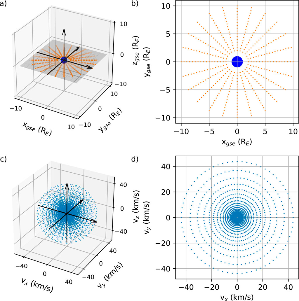
Figure 1. MATE spatial and velocity grids. (A) Spatial grids in 3D GSE coordinates, (B) spatial grids on the GSE equatorial plane, (C) sample velocity grids in 3D velocity space, (D) sample velocity grids on the plane where $v_z=0$. The actual velocity grids used in this study are more densely populated.

The geocoronal observations from NASA’s Two Wide-angle Imaging Neutral-atom Spectrometers (TWINS) mission recently revealed exospheric variability during a geomagnetic storm. Bailey and Gruntman (2013) showed an N_H increase of 6–17% in a region of 3–8 R_E radial distances by calculating the exospheric density inversely from the TWINS geocorona observations of five geomagnetic storms. Zoennchen et al. (2017) also reported a similar density increase of 9%–23% in the same radial distances by considering the variation of the geocoronal column brightness as a proxy of column H-density variation. Their analysis of eight geomagnetic storms showed that the enhancement of geocoronal emission tends to decrease with increasing storm intensity, parameterized by minimum Dst, implying a complex response of our exosphere to a geomagnetic storm. Cucho-Padin and Waldrop (2019) presented further interesting storm-time behaviors by applying a tomographic method to the TWINS storm-time geocorona observations. They reported that N_H enhances by ∼15% at 3R_E geocentric distance soon after the minimum Dst, and the density enhancement propagates outward. Despite observational evidence of storm-time exosphere density variability, there has been no modeling study to decipher this storm-time behavior.

In this paper, we develop a new dynamic model of the terrestrial hydrogen exosphere that utilizes physics-based exobase conditions from the Thermosphere–Ionosphere–Mesosphere–Electrodynamics General Circulation Model (TIMEGCM). We then investigate how the time-varying exobase conditions influence exospheric H density before, during, and after a geomagnetic storm from 12 to 18 June 2008. We compare the model results with the TWINS N_H estimates of the same storm from Cucho-Padin et al. (2023) and investigate the physical mechanisms responsible for the observed storm-time exospheric behaviors. Finally, we conclude our research and remark on future model development plans to support the upcoming spacecraft missions.

2 Models

2.1 Thermosphere – ionosphere – mesosphere – electrodynamics general circulation model (TIMEGCM)

The NCAR TIMEGCM (Roble and Ridley, 1994) is a first-principles upper atmospheric general circulation model that solves the fully coupled, nonlinear, hydrodynamic, thermodynamic, and continuity equations of the neutral gas self-consistently with the ion energy, ion momentum, and ion continuity equations. It utilizes a spherical coordinate system fixed with respect to the rotating Earth, with latitude and longitude as the horizontal coordinates and pressure surface as the vertical coordinate. In the configuration used for this study, it has a horizontal resolution of 5° × 5°. The pressure interfaces are defined as z_p = ln (P₀/P), and P₀ is a reference pressure at $5\times {10}^{-4}\mu bar$. The model has 49 pressure surfaces covering the altitude range from ∼30 km to ∼600 km, with z_p ranging from −17 to +7 (∼30–600 km depending on solar activity) and a vertical resolution of one-half scale height. The external forcings of the TIMEGCM are solar irradiance, parameterized using the F_10.7 index by default (Solomon and Qian, 2005); auroral electron precipitation (Roble and Ridley, 1987) and ionospheric convection driven by the magnetosphere-ionosphere current system (Heelis et al., 1982); and the amplitudes and phases of diurnal and semi-diurnal migrating tides from the lower atmosphere (Hagan and Forbes, 2002; Hagan and Forbes, 2003). The model output includes neutral, ion, and electron temperature, neutral winds and plasma drifts, major and minor species mixing ratios, electron density, geopotential height of model pressure surfaces, and electrical potential. The model can also output many diagnostic variables, such as geometric height, mass density, Joule heating, infrared radiative cooling rates, conductivity, electric field, the peak altitude, and density of the ionospheric F2 region, and ionospheric currents. Additional diagnostic and derived parameters can be calculated by standard output processing software.

2.2 Model for analyzing terrestrial exosphere (MATE)

MATE is a dynamic model of the terrestrial hydrogen exosphere, developed based on the Liouville Theorem Particle Tracer (LTPT) introduced by Connor et al. (2012), Connor et al. (2015). LTPT is designed to analyze cusp ion energy dispersions for studying magnetopause reconnection. MATE differs from LTPT because MATE targets neutral hydrogen atoms instead of cusp ions, and particle trajectories are governed by gravity, not electromagnetic forces. The MATE model comprises two main components: 1) neutral hydrogen tracer and 2) exospheric density calculator.

2.2.1 Neutral hydrogen tracer

We employ 2D spatial grids and 3D velocity grids to analyze the time-varying exospheric density on the ecliptic plane during a geomagnetic storm. The spatial grids are spaced at intervals of 0.5 R_E between 2 and 10 R_E radial distance with an angular resolution of 15° in GSE longitude. Figures 1A, B display the spatial grids in 3D GSE coordinates (left) and on the GSE equatorial plane (right). It is important to note that users can introduce 3D spatial grids in the MATE simulation and expand them to cover any region of interest above the exobase altitude of 500 km, with a spatial resolution finer than 0.5 R_E and 15° longitude/latitude. This study specifically selects the 2D spatial grids on the ecliptic plane because we are interested in this region.

The velocity grids consist of a total of 1,248,478 grids, encompassing 121 logarithmically spaced energy channels ranging from 0.0025 to 10 eV — corresponding to 121 velocity magnitudes ranging from ∼700 m/s to ∼40 km/s. These channels cover the typical energy of exobase hydrogen, ∼0.1 eV or 1000 K (Qin and Waldrop, 2016). Additionally, there are 10,318 velocity directions, evenly spaced to have an equal solid angle of ∼0.001 steradians, which provides a finite resolution of 2° in $\theta$ and a varying resolution in $\phi$. Figures 1C, D show samples of velocity grids in the 3D velocity space and on the plane of $v_z=0$ for easier viewing of the velocity grids. The actual velocity grids used in this study are much more densely populated.

The neutral hydrogen tracer tracks a hydrogen atom backward in time from a designated point in the exosphere to the exobase at an altitude of 500 km by integrating equations of motion (1) in Geocentric Solar Ecliptic coordinates (GSE), considering only gravitational force:

$\mathit{F}=m\mathit{a}=m\mathit{g},\mathit{a}=\frac{d\mathit{v}}{dt},\mathit{v}=\frac{d\mathit{r}}{dt}(1)$

where F is the gravitational force, m is the mass of a hydrogen atom, g is the acceleration due to the Earth’s gravity, and a, v, and r are the acceleration, velocity, and position vectors, respectively. Using the 4^th-order Runge-Kutta method, the tracer calculates the position and velocity of a hydrogen atom for up to 50 days, with an early stop enabled if the hydrogen reaches the exobase (the source region of terrestrial hydrogen atoms) or a geocentric distance of 100 R_E, where we assume a source region of extraterrestrial hydrogen atoms. Figure 2 shows example trajectories of exospheric hydrogen atoms launched from an exospheric point $\mathit{r}$ (a red dot) at time $t$. The orange and blue lines display the trajectories of hydrogen atoms originating from the exobase and interplanetary space, respectively. The blue dots indicate the exobase footprints of the exobase-originating hydrogens. The green lines represent the trajectories of atoms that do not reach either the exobase or interplanetary space within the 50-day tracing period.

Figure 2

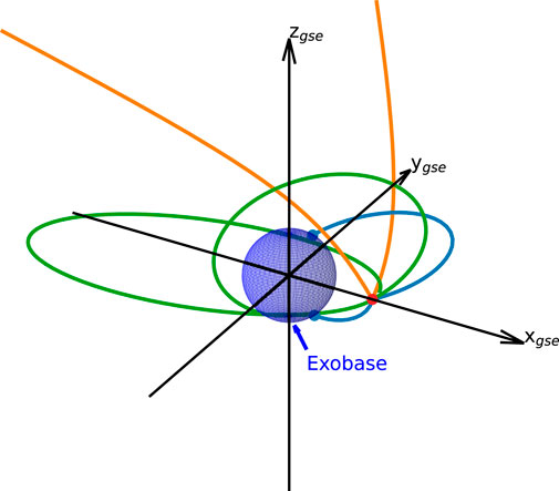
Figure 2. Example trajectories of neutral hydrogen atoms launched from an exospheric point of interest (red point) and traced backward in-time by the MATE neutral hydrogen tracer. The blue and orange lines represent the trajectories of hydrogen atoms originating from the exobase and interplanetary space, while the green lines represent the trajectories of satellite hydrogen atoms. The blue sphere represents the exobase at a 500 km altitude, and the blue points indicate the exobase footprints of the hydrogen atoms.

To cover the spacious exosphere above 2R_E radial distance, our exosphere model adopts a computationally efficient backward tracing technique instead of a forward tracing method that requires launching numerous hydrogen atoms from the exobase to the exosphere until statistically strong density samples are gathered across the entire exosphere region of our interest (2–10 R_E radial distance). It is worth noting that by selecting the GSE coordinates, MATE does not need to account for Coriolis and centrifugal forces caused by the Earth’s rotation around its axis as these forces are fictitious forces and only arise in geographic coordinates, not in GSE coordinates. Additionally, while similar fictitious forces exist in the GSE coordinates due to the Earth’s revolution around the Sun, their impact is negligible for the time scale of our interest (less than 7 days).

For this storm study, the tracer launches approximately 1.2 million hydrogen atoms every hour at each spatial grid along a Sun-Earth line. Since the gravitational force exhibits spherical symmetry, the trajectories of the hydrogen atoms are also symmetric. To alleviate computational burden, we rotate the hydrogen trajectories calculated along the Sun-Earth line by 15° increments around the Z_gse axis and utilize the rotated results for the remaining spatial grids on the ecliptic plane.

2.2.2 Exospheric density calculator

The density calculator treats each hydrogen atom traced in Section 2.2.1 as a parcel of hydrogen and calculates a Phase Space Density (PSD) for each hydrogen parcel based on its source region. If a hydrogen atom reaches a radial distance of 100 R_E, it is assumed to be extraterrestrial hydrogen. The Lyman-$\mathrm{\alpha }$ emission from interplanetary space is much lower than that from the geocorona (e.g., Kameda et al., 2017). The PSDs of extraterrestrial hydrogen atoms are expected to be negligibly smaller than those of exobase-originating hydrogen atoms and are therefore set to zero. If a hydrogen atom remains in the exosphere without reaching the exobase or 100 R_E for 50 days, it is assumed to be an orbiting particle. These particles are typically created by collisions and may contribute to the exospheric density. However, the current MATE model neglects these particles and sets their PSDs to zero. Their contribution will be addressed in a future study. Consequently, the density calculator only estimates the PSDs of hydrogen atoms originating from the exobase.

We first assume that hydrogen at the exobase follows the Maxwellian velocity distribution. The phase space density of an exobase-originating hydrogen ($f$) will be calculated using the following Equation 2 (Baumjohann and Treumann, 1997):

$f\left(r_b,v_b,t_b\right)=n_b\left({\mathit{r}}_b,t_b\right){\left[\frac{m_H}{2\pi k_b{T}_b\left({\mathit{r}}_b,t_b\right)}\right]}^{\frac{3}{2}}\mathit{exp}\left[-\frac{{m_H\left\{{\mathit{v}}_{\mathit{b}}-{\mathit{V}}_b\left({\mathit{r}}_b,t_b\right)\right\}}^2}{2k_b{T}_b\left({\mathit{r}}_b,t_b\right)}\right](2)$

where ${\mathit{r}}_b$, ${\mathit{v}}_{\mathit{b}}$, and $t_b$ are the location, velocity, and time of the hydrogen at the exobase, $k_b$ is Boltzmann constant, and $n_b$, ${\mathit{V}}_b$, and $T_b$ represent the exobase conditions, i.e., hydrogen number density, drift velocity, and temperature at ${\mathit{r}}_b$ and $t_b$. The neutral hydrogen tracer provides ${\mathit{r}}_b$, ${\mathit{v}}_{\mathit{b}}$, and $t_b$ of an exobase-originating hydrogen, and the TIMEGCM upper atmosphere model provides time-varying exobase conditions (i.e., $n_b$, ${\mathit{V}}_b$, and $T_b$) throughout a geomagnetic storm. The TIMEGCM grid resolution used in this study is 5° longitude and 5° latitude in the geographic coordinates, and the output cadence is 5 min. We convert the TIMEGCM grids into GSE coordinates and use linear interpolation to obtain the exobase conditions at ${\mathit{r}}_b$ and $t_b$.

We then assume that the PSD calculated at the exobase, i.e., $f\left({\mathit{r}}_{\mathit{b}},{\mathit{v}}_{\mathit{b}},t_b\right)$, is conserved along a trajectory from the exobase to the exosphere. Using Liouville’s theorem, we obtain the PSD of an exobase-originating hydrogen at $\mathit{r}$, $\mathit{v}$, and $t$ using Equation 3:

$f\left(\mathit{r},\mathit{v},t\right)\approx f\left({\mathit{r}}_{\mathit{b}},{\mathit{v}}_{\mathit{b}},t_b\right).(3)$

Finally, we determine the exospheric hydrogen density ($N_H$) at $\mathit{r}$ and $t$ by integrating the PSDs of all traced hydrogen over velocity space as seen in Equation 4.

$N_H\left(\mathit{r},t\right)=\int f\left(\mathit{r},\mathit{v},t\right)d\mathit{v}.(4)$

Figure 3 illustrates the methodology of the MATE exospheric density calculator. Figure 3A shows the trajectories of two exospheric hydrogen atoms, P1 and P2, launched from $\left(\mathit{r},t\right)$ with two different velocities, ${\mathit{v}}_{\mathbf{1}}$ and ${\mathit{v}}_{\mathbf{2}}$. The tracer calculates when, where, and at what velocity the two atoms start their journey from the exobase to the exospheric point $\left(\mathit{r},t\right)$. P1 departs from the exobase location ${\mathit{r}}_{\mathit{b}\mathbf{1}}$ at time $t_{b1}$ with velocity ${\mathit{v}}_{b1}$, while P2 departs from the exobase location ${\mathit{r}}_{\mathit{b}\mathbf{2}}$ at time $t_{b2}$ with velocity ${\mathit{v}}_{b2}$. Although P1 and P2 arrive at the same exospheric point $\mathit{r}$ at the same time $t$, their departure from the exobase occurs at different locations and times with different velocities. Then, the density calculator obtains time-varying exobase conditions from TIMEGCM — namely, hydrogen atom density ($n_b$), neutral wind velocity (${\mathit{V}}_b$), and neutral temperature ($T_b$). Figure 3B illustrates two different exobase conditions at $t_{b1}$ and $t_{b2}$, providing $n_{b1}$, ${\mathit{V}}_{b1}$, and $T_{b1}$ at $\left({\mathit{r}}_{\mathit{b}\mathbf{1}},t_{b1}\right)$ for P1 and $n_{b2}$, ${\mathit{V}}_{b2}$, and $T_{b2}$ at $\left({\mathit{r}}_{\mathit{b}\mathbf{2}},t_{b2}\right)$ for P2. Finally, the density calculator estimates PSDs using the Maxwellian velocity distribution in Equation 2, obtaining $f_{b1}\left({\mathit{r}}_{\mathit{b}\mathbf{1}},{\mathit{v}}_{\mathit{b}\mathbf{1}},t_{b1}\right)$ for P1 and $f_{b2}\left({\mathit{r}}_{\mathit{b}\mathbf{2}},{\mathit{v}}_{\mathit{b}\mathbf{2}},t_{b2}\right)$ for P2. Assuming no collisions throughout their journey from the exobase to the exosphere, their PSDs calculated at the exobase are conserved along the trajectories: ${f_1\left(\mathit{r},{\mathit{v}}_{\mathbf{1}},t\right)\approx f}_{b1}\left({\mathit{r}}_{\mathit{b}\mathbf{1}},{\mathit{v}}_{\mathit{b}\mathbf{1}},t_{b1}\right)$ and ${f_2\left(\mathit{r},{\mathit{v}}_{\mathbf{2}},t\right)\approx f}_{b2}\left({\mathit{r}}_{\mathit{b}\mathbf{2}},{\mathit{v}}_{\mathit{b}\mathbf{2}},t_{b2}\right)$, as seen in Figure 3C. Adopting this Liouville mapping, the density calculator determines the PSDs of all exospheric hydrogen atoms originating from the exobase and integrates them over velocity space for calculating the exospheric hydrogen density (Equation 4).

Figure 3

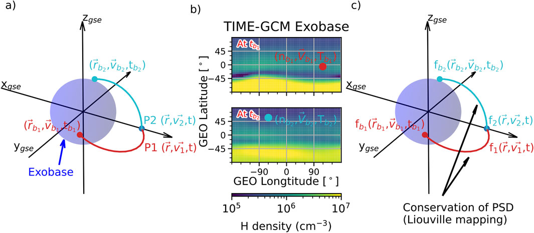
Figure 3. Methodology of the MATE exospheric density calculator. (A) Trajectories of two hydrogen atoms, P1 (red) and P2 (cyan), launched from the exospheric point $\mathit{r}$ at time $t$. Their phase-space-time coordinates at the exobase are $\left({\mathit{r}}_{\mathit{b}\mathbf{1}},{\mathit{v}}_{\mathit{b}\mathbf{1}},t_{b1}\right)$ and $\left({\mathit{r}}_{\mathit{b}\mathbf{2}},{\mathit{v}}_{\mathit{b}\mathbf{2}},t_{b2}\right)$. (B) TIME-GCM exobase conditions at $t_{b1}$ (top) and $t_{b2}$ (bottom). Exobase hydrogen atom density, neutral wind, and neutral temperature at the exobase footprints of P1 and P2 (red and cyan points) are identified as $\left(n_{b1},{\mathit{V}}_{\mathit{b}\mathbf{1}},t_{b1}\right)$ and $\left(n_{b2},{\mathit{V}}_{\mathit{b}\mathbf{2}},t_{b2}\right)$. These conditions are used to calculate phase-space densities of P1 and P2 at the exobase. (C) Liouville mapping of phase-space densities between the exobase and the exosphere: $f_1\left(\mathit{r},{\mathit{v}}_{\mathbf{1}},t\right)=f_{b1}\left({\mathit{r}}_{\mathit{b}\mathbf{1}},{\mathit{v}}_{\mathit{b}\mathbf{1}},t_{b1}\right)$ and $f_2\left(\mathit{r},{\mathit{v}}_{\mathbf{2}},t\right)=f_{b2}\left({\mathit{r}}_{\mathit{b}\mathbf{2}},{\mathit{v}}_{\mathit{b}\mathbf{2}},t_{b2}\right)$.

2.3 Model limitation and merit

The current version of MATE is relatively simple. It considers only gravitational force and assumes no collision of hydrogen along their journey between the exobase and the exosphere (i.e., Liouville’s Theorem). Additionally, only ballistic and escaping hydrogens of the exobase origin determine N_H in our model. Hydrogens in orbit and from interplanetary space play no role in the density determination (i.e., producing zero phase-space densities). Furthermore, the current MATE model omits other physical processes: solar radiation pressure that pushes the terrestrial exosphere anti-sunward; neutral-neutral collision that modifies hydrogen trajectories but is likely negligible in the outer exosphere of our interest; neutral-plasma collision that energizes neutral hydrogen to 1 eV–1 MeV via charge exchange with plasmaspheric and ring current ions; and photoionization that ionizes a hydrogen after its long stay in the exosphere.

However, when MATE is coupled with the TIMEGCM exobase conditions, it becomes a powerful tool to study storm-time exospheric variability caused by dynamic exobase conditions. Since the gravitational force does not change during a geomagnetic storm, it is the exobase condition that modifies exospheric density throughout a storm. In other words, hydrogen atom density, drift velocity, and temperature at the exobase determine the number of escaping and ballistic hydrogen atoms entering the exosphere. This mobility of exobase hydrogen atoms is the primary physical process in the MATE model that distributes hydrogen across the exosphere. Global circulation models like TIMEGCM have significantly improved in the past decade, providing first-principles calculations of exobase conditions during an active time. Therefore, our storm-time exosphere study is unique and advanced compared to previous modeling efforts that use steady exobase conditions (e.g., Hodges, 1994; Baliukin et al., 2019).

It is worth noting a few points about the MATE-TIMEGCM coupling. The coupling is one-way: MATE utilizes the output of TIMEGCM, but TIMEGCM does not incorporate information from MATE. Additionally, the height of the exobase changes during a geomagnetic storm, increasing in altitude due to the increase in atmospheric heating. For simplicity and convenience, we select a fixed exobase altitude of 500 km, with the assumption that the Maxwellian velocity distribution is marginally accepted at this altitude. The impact of two-way coupling and variable exobase height will be addressed in future research.

3 Model results and discussion

We select the period from 12 to 18 June 2008, which includes a minor geomagnetic storm on 14-15 June 2008. Previous studies (Zoennchen et al., 2017; Cucho-Padin and Waldrop, 2019; Cucho-Padin et al., 2023) have repeatedly reported that the TWINS Lyman-$\mathrm{\alpha }$ instruments observed enhanced geocorona emission during this storm. We conduct the TIMEGCM simulation during 12–18 June 2008 and extract the exobase conditions every 5 minutes.

During a geomagnetic storm, powerful energy enters from the magnetosphere into the high-latitude upper atmosphere in the form of auroral precipitation and Poynting flux. This energy subsequently heats and expands the upper atmosphere, initiating a new global circulation of the neutral atmosphere. Consequently, thermospheric mass density, both horizontal and vertical neutral winds, and temperature enhance during a geomagnetic storm (e.g., Richmond and Lu, 2000; Fuller-Rowell et al., 2007). On the other hand, lighter atoms such as hydrogen atoms behave differently. Qian et al. (2018) reported from the WACCM-X whole atmosphere simulation that atomic hydrogen density in the upper atmosphere (above 150 km altitude) responds inversely to thermospheric temperature. The upper atmospheric hydrogen density is lower during the day than at night, lower in summer than in winter, and lower at solar maximum than at solar minimum. Although Qian et al. (2018) does not cover a geomagnetic storm, a similar behavior (i.e., lower density during a storm than during quiet days) was suggested by Qin et al. (2017), who reported a reduced hydrogen density in the upper atmosphere during two geomagnetic storms by analyzing the geocoronal observations from the Thermosphere Ionosphere Mesosphere Energetics and Dynamics (TIMED) satellite.

Figure 4 compares the TIMEGCM exobase conditions during a quiet time at 11 UT on 14 June 2008 (left) and during a storm time at 11 UT on 15 June 2008 (right). TIMEGCM reveals a well-known hemispheric asymmetry in the exobase conditions caused by the solstice: for example, denser hydrogen density in the winter hemisphere and higher temperature in the summer hemisphere. During a storm, the exobase hydrogen density (top) decreases while the temperature (middle) increases, as demonstrated by the global averages of these two parameters (see the lower left corner of each plot). This storm impact is particularly noticeable in high latitude regions. Additionally, both horizontal (bottom, vectors) and vertical (bottom, colors) winds intensify at high latitudes above 60° geographic latitude where strong Joule heating typically occurs due to enhanced high-latitude forcings. The global average of TIMEGCM exobase hydrogen density is $2-5\times {10}^6$ cm⁻³, higher than $\sim 3\times {10}^5$ cm⁻³ predicted for this time of year by the NRLMSIS2.0 empirical whole atmosphere model (Emmert et al., 2021). However, TIMEGCM faithfully and effectively captures the overall response of the upper atmosphere to a geomagnetic storm. This dynamic variation of the upper atmosphere influences exobase conditions and alters the number of ballistic and escaping hydrogen atoms, consequently modifying exospheric density throughout the geomagnetic storm.

Figure 4

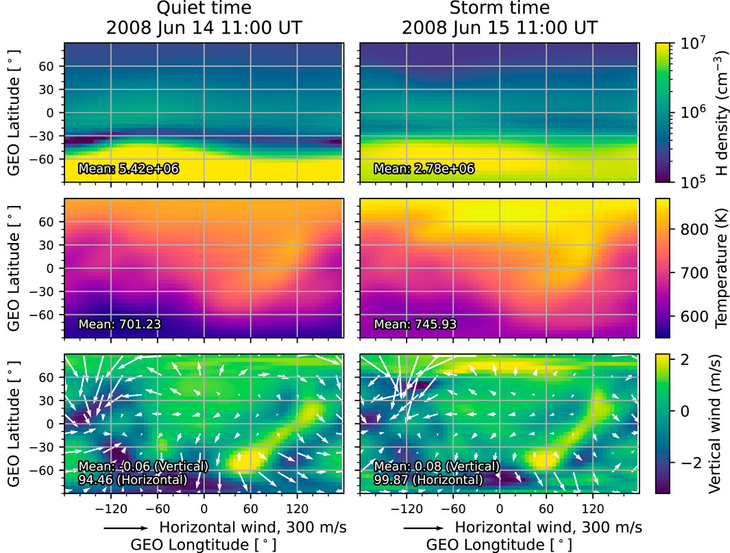
Figure 4. The TIME-GCM exobase conditions in geographic coordinates: hydrogen number density (top), neutral temperature (middle), and neutral wind (bottom) for a quiet time at 11 UT on 14 June 2008 (left) and a storm time at 11 UT on 15 June 2008 (right). The global average of each parameter is labeled in the lower left corner of each plot. In the bottom panel, horizontal winds are represented by vectors, while vertical winds are displayed using color gradients.

We conduct the MATE simulation for the period from 12–18 June 2008 using the TIMEGCM exobase conditions and extract an hourly exospheric neutral density. Figure 5 presents the simulation results. The left two panels show hydrogen density on the ecliptic equatorial plane during a quiet time at 11 UT on 14 June 2008 and a storm time at 11 UT on 15 June 2008. The right panel displays the relative percent difference between storm- and quiet-time densities. At this storm time, hydrogen density increases across the entire exosphere with the strongest percent increase in the afternoon sector. The relative density enhancement ranges from ∼22% at ∼2 R_E distance to ∼63% at ∼7 R_E radial distances. Although the 20% increase at 2 R_E may sound small, the actual density increase is much stronger at this distance, considering that the hydrogen number density at 2 R_E is 10^3.6 ∼ 10⁴ cm⁻³, while the density at 7 R_E is 10^1.6 ∼ 10² cm⁻³.

Figure 5

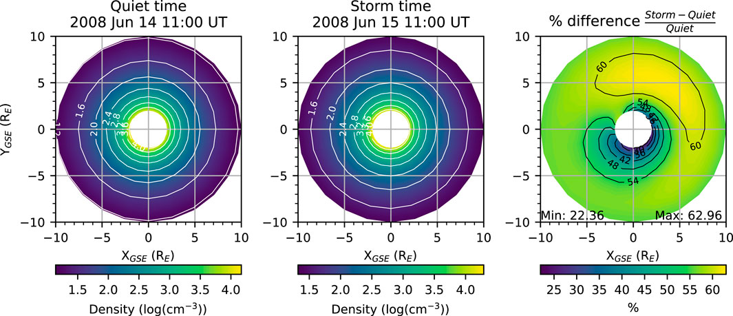
Figure 5. The MATE simulation results. The left and middle panels display the exospheric hydrogen density on an ecliptic equatorial plane during a quiet time at 11 UT on 14 June 2008 and during a storm time at 11 UT on 15 June 2008, respectively. The right panel displays the relative percent difference between the storm - and quiet-time densities.

We compared our model results with the TWINS N_H estimates of Cucho-Padin et al. (2023). Cucho-Padin et al. (2023) extracted the time variation of global N_H profiles from TWINS Lyman-$\mathrm{\alpha }$ observations using 4D tomography. Their N_H profiles explained 85–97% of the geocoronal intensity observed by TWINS and were further smoothed to calculate a general trend of N_H variability by applying Fourier-based interpolation to only the N_H data points of above 90% accuracy obtained when TWINS provides abundant Lyman-$\mathrm{\alpha }$ measurements for successful tomography. We used this general N_H trend as ground truth but with caution, acknowledging that the TWINS N_H estimates are not in situ measurements and thus may have limitations in capturing all the details of N_H variation.

Figure 6 shows Dst (top), Kp (middle), and the temporal evolution of N_H at 4 radial distances along a dayside Sun-Earth line (bottom). Solid lines represent N_H from the MATE model, while dashed lines represent the general trend of TWINS N_H estimates from Cucho-Padin et al. (2023). Vertical black lines indicate the quiet and storm times shown in Figures 4, 5. Dst increases to 35 nT at 14 UT on 14 June 2008 during the sudden storm commencement and then reaches its minimum value of −41 nT at 5 UT on 15 June 2008. The TWINS data show enhanced N_H in the region of 3.15–6.75 R_E soon after Dst reaches its minimum. The MATE model also captures the storm-time exospheric density enhancement at similar times, suggesting that the increased mobility of exobase hydrogen atoms, caused by atmospheric heating, is a dominant factor in the N_H enhancement observed by TWINS.

Figure 6

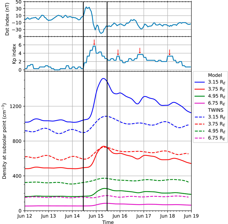
Figure 6. Time evolution of exospheric hydrogen density during 12 – 19 June 2008. Dst (top), Kp (middle), H density at four subsolar points from 3.15 to 6.75 R_E (bottom) are displayed. Solid density lines are the MATE results, while dashed lines are the TWINS estimates from Cucho-Padin et al. (2023). Two vertical black lines indicates the quiet and storm times shown in Figures 4, 5.

MATE N_H exhibits three additional enhancements near 0 UT on 16 June 2008, 0 UT on 17 June 2008, and 6 UT on 18 June 2008, occurring 3–6 h after the Kp peaks (see red arrows in Figure 6). These enhancements are more evident at a distance between 3.15 and 4.95 R_E. In contrast, TWINS N_H shows only 1-2 additional enhancements at different times after 11 UT on 15 June 2008. TIMEGCM drives the upper atmosphere with Kp-dependent high-latitude forcings (Heelis et al., 1982; Roble and Ridley, 1987). The timing and intensity of these high-latitude forcings in the TIMEGCM model may not perfectly align with reality. Additionally, MATE is a simplified model as it only considers gravitational force and assumes no collisions along the trajectory of a hydrogen atom. These factors may contribute to the model-data discrepancy of storm-time and after-storm N_H enhancements. Despite these limitations, the coupling of the MATE model with TIMEGCM exobase conditions provides valuable insight: the dynamic response of the upper atmosphere to high-latitude forcings can lead to multiple N_H enhancements throughout and after a storm. As Kp reaches each peak, TIMEGCM injects stronger magnetospheric energy into the high-latitude regions, intensifying upper atmospheric heating and subsequently increasing exospheric densities several hours after the Kp peaks. This delayed exospheric response occurs partially due to the travel time of hydrogen atoms from the exobase to the exosphere.

While our model reproduces higher N_H during and after a storm compared to quiet times, the magnitude of modeled N_H does not match the TWINS estimates. This discrepancy is understandable considering the limited physics used in the MATE model and the elevated exobase hydrogen atom density of TIMEGCM compared to the empirical predictions of NRLMSIS2.0. In addition to these model limitations, we can explore other physical mechanisms that may contribute to this density discrepancy. For example, our model shows higher density at 3.15 R_E and lower density at higher radial distances than the TWINS estimates. This discrepancy pattern is potentially due to neutral-ion charge exchange in the plasmasphere and ring current. By exchanging electrons with ions in these magnetospheric regions, ∼0.1 eV hydrogen atoms of exobase origin are converted to 1 eV–100 keV hydrogen atoms (Qin and Waldrop, 2016), redistributing hydrogens across the exosphere. Additionally, solar radiation pressure may increase the lower MATE N_H at higher radial distances, bringing it closer to the TWINS N_H. Beth et al. (2016) reported that dayside exospheric density can increase up to ∼50% by considering solar radiation pressure in addition to gravity. The neutral – ion charge exchange and solar radiation pressure, in addition to the intrinsic limitations of MATE and TIMEGCM (e.g., the assumption of a Maxwellian distribution of exobase hydrogens in MATE and imperfect representations of high-latitude forcings in TIMEGCM), may contribute to this model-data discrepancy, motivating further model improvements.

4 Summary and concluding remarks

Recent studies of TWINS Lyman-$\mathrm{\alpha }$ observations (Bailey and Gruntman, 2013; Zoennchen et al., 2017; Cucho-Padin and Waldrop, 2019; Cucho-Padin et al., 2023) have reported variations in geocorona intensity during geomagnetic storms, indicating a dynamic response of the terrestrial exosphere to space weather. The variability in exospheric density can significantly impact inner magnetospheric dynamics, as denser neutrals lead to increased neutral-plasma charge exchange in the ring current, thereby accelerating energy decays. However, previous models (e.g., Hodges, 1994; Baliukin et al., 2019) have not addressed this continuously varying exospheric behavior.

We developed a Model for Analyzing Terrestrial Exosphere (MATE) to study the storm-time variation in exospheric density and its underlying physical mechanisms. MATE traces test hydrogen atoms backward in time from a chosen point in the exosphere to the exobase under gravity. It then estimates phase-space densities of these hydrogen atoms based on their velocity and the conditions of their exobase origins, making two key assumptions: 1) a Maxwellian distribution of exobase hydrogen atoms and 2) the conservation of the phase-space densities throughout their journey between the exobase and the exosphere. MATE leverages the TIMEGCM upper atmosphere model to obtain physics-based, dynamic exobase conditions during a geomagnetic storm. Finally, MATE calculates exospheric hydrogen density by integrating the phase-space densities over velocity space. Since the gravitational force remains constant over a geomagnetic storm, the changing exobase conditions are found to be the primary contributor to the storm-time exospheric density variation in the MATE model.

We simulated exospheric neutral density within the radial distance of 2–10 R_E during 12–18 June 2008, and compared the results with TWINS N_H estimates from Cucho-Pardin et al. (2023). MATE captures the enhanced exospheric density soon after Dst reaches its minimum, as observed in the TWINS N_H estimates. Strong high-latitude forcing during a geomagnetic storm heats the upper atmosphere and the exobase, increasing the number of ballistic and escaping hydrogen atoms entering the exosphere and thereby enhancing N_H with a delayed response due to the travel time of hydrogen atoms from the exobase to the exosphere. Although MATE and TWINS N_H show good agreement in the storm-time density enhancement near 11 UT on 15 June 2008, their N_H magnitudes mismatch. This density discrepancy results from various mechanisms: the inherent limitations of MATE and TIMEGCM, omission of neutral-ion charge exchange in the plasmasphere and ring currents, and exclusion of solar radiation pressure.

A series of improvements to the MATE model are planned for the near future. Firstly, we intend to incorporate additional force terms, such as solar radiation pressure and the Coriolis force caused by the Earth’s revolution around the Sun, into the neutral hydrogen tracer. Additionally, we will solve the Boltzmann equations, considering loss and source terms resulting from photoionization and charge-exchanges between exospheric hydrogen atoms and ring current ions. Finally, we will utilize the exobase conditions of WACCM-X, a more advanced global circulation model than TIMEGCM (Liu et al., 2018), to achieve a more realistic range of the exobase hydrogen atom density. With these improvements, MATE will become an essential tool for analyzing exosphere density data from the forthcoming NASA Carruthers Geocorona Observatory (expected to launch in 2025), thereby revealing the physical drivers of global exosphere density structure and temporal variability.

The storm-time N_H enhancement also provides interesting insights for scheduled missions such as Lunar Environment heliospheric X-ray Imager (LEXI; Walsh et al., 2024) and Solar wind – Magnetosphere – Ionosphere Link Explorer (SMILE; Branduardi-Raymont et al., 2018). LEXI and SMILE will observe the dayside magnetosheath and cusps in soft X-rays after their respective launches in 2024 and 2025, aiming to understand the global interaction between solar wind and magnetosphere. Soft X-rays are emitted when highly charged solar wind ions, such as O⁷⁺, exchange electrons with exospheric hydrogen atoms and subsequently relax to a lower energy state. Strong solar wind ion fluxes and/or enhanced exospheric hydrogen density increases soft X-ray emissivity in the magnetosheath and cusps (Connor et al., 2021).

Our MATE model shows that the hydrogen density at the 10 R_E subsolar point (i.e., near the subsolar magnetopause) increases soon after the storm main phase and remains elevated for several days. SMILE and LEXI may be able to detect strong soft X-ray emissions not only during the initial phase of a storm when solar wind fluxes intensify but also throughout the remainder of the storm period due to the enhanced exospheric density. SMILE and LEXI are anticipated to capture high-quality soft X-ray images of the dayside magnetosheath and cusps throughout a geomagnetic storm, thereby providing invaluable data for studying the interaction between solar wind and geospace.

Data availability statement

The datasets presented in this study can be found in online repositories. The names of the repository/repositories and accession number(s) can be found below: https://drive.google.com/drive/folders/1aHU03x29vrlOMUwZ3vOPLsqKJiXsIqBn?usp&=sharing.

Author contributions

HC: Conceptualization, Data curation, Formal Analysis, Funding acquisition, Investigation, Methodology, Project administration, Resources, Software, Supervision, Validation, Visualization, Writing–original draft, Writing–review and editing. JJ: Data Curation, Formal Analysis, Validation, Visualization, Writing–original draft, Writing–review and editing. LQ: Methodology, Writing–original draft, Writing–review and editing. ES: Conceptualization, Writing–original draft, Writing–review and editing. GC-P: Validation, Writing–original draft, Writing–review and editing. MC: Conceptualization, Writing–original draft, Writing–review and editing. S-YL: Methodology, Writing–original draft, Writing–review and editing.

Funding

The author(s) declare that financial support was received for the research, authorship, and/or publication of this article. This work was supported by the NASA Heliophysics Theory, Modeling, and Simulations (H-TMS) Program under Grant WBS 791926.02.04.02.26, the NASA Heliophysics United States Participating Investigator Program under Grant WBS 516741.01.24.01.03, and the NASA Lunar Surface Instrument and Technology Payloads program under Grant 80MSFC20C0019. ES was supported by the NASA H-TMS Program under Grant 80NSSC20K1278.

Acknowledgments

The authors acknowledge the support from the International Space Science Institute on the ISSI team #492, titled “The Earth’s Exosphere and its Response to Space Weather.”

Conflict of interest

The authors declare that the research was conducted in the absence of any commercial or financial relationships that could be construed as a potential conflict of interest.

Publisher’s note

All claims expressed in this article are solely those of the authors and do not necessarily represent those of their affiliated organizations, or those of the publisher, the editors and the reviewers. Any product that may be evaluated in this article, or claim that may be made by its manufacturer, is not guaranteed or endorsed by the publisher.

References

Bailey, J., and Gruntman, M. (2013). Observations of exosphere variations during geomagnetic storms. Geophys. Res. Lett. 40, 1907–1911. doi:10.1002/grl.50443

CrossRef Full Text | Google Scholar

Baliukin, I., Bertaux, J.-L., Qu merais, E., Izmodenov, V., and Schmidt, W. (2019). SWAN/SOHO Lyman-α mapping: the hydrogen geocorona extends well beyond the Moon. J. Geophys. Res. Space Phys. 124, 861–885. doi:10.1029/2018JA026136

CrossRef Full Text | Google Scholar

Baumjohann and Treumann (1997). Basic space plasma physics. World Scientific Pub Co. Incorp. doi:10.1142/p015

CrossRef Full Text | Google Scholar

Beth, A., Garnier, P., Toublanc, D., Dandouras, I., and Mazelle, C. (2016). Theory for planetary exospheres: II. Radiation pressure effect on exospheric density profiles. Icarus 266 (2016), 423–432. doi:10.1016/j.icarus.2015.08.023

CrossRef Full Text | Google Scholar

Beth, A., Garnier, P., Toublanc, D., Dandouras, I., Mazelle, C., and Kotova, A. (2014). Modeling the satellite particle population in the planetary exospheres: application to Earth, Titan and Mars. Icarus 227 (2014), 21–36. doi:10.1016/j.icarus.2013.07.031

CrossRef Full Text | Google Scholar

Branduardi-Raymont, G., Wang, C., Escoubet, C. P., Adamovic, M., Agnolon, D., Berthomier, M., et al. (2018). SMILE definition study report (red book). ESA/SCI. Available at: https://sci.esa.int/web/smile/-/61194-smile-definition-study-report-red-book.

Google Scholar

Connor, H. J., Raeder, J., and Trattner, K. J. (2012). Dynamic Modeling of cusp ion structures. J. Geophys. Res. 117, A04203. doi:10.1029/2011JA017203

CrossRef Full Text | Google Scholar

Connor, H. K., Raeder, J., Sibeck, D. G., and Trattner, K. J. (2015). Relation between cusp ion structures and dayside reconnection for four IMF clock angles: OpenGGCM-LTPT results. J. Geophys. Res. Space Phys. 120, 4890–4906. doi:10.1002/2015JA021156

CrossRef Full Text | Google Scholar

Connor, H. K., Sibeck, D. G., Collier, M. R., Baliukin, I. I., Branduardi-Raymont, G., Brandt, P. C., et al. (2021). Soft X-ray and ENA imaging of the earth's dayside magnetosphere. J. Geophys. Res. Space Phys. 126, e2020JA028816. doi:10.1029/2020JA028816

PubMed Abstract | CrossRef Full Text | Google Scholar

Cucho-Padin, G., Godinez, H., Waldrop, L., Baliukin, I., Bhattacharyya, D., Sibeck, D., et al. (2023). A new approach for 4-D exospheric tomography based on optimal interpolation and Gaussian markov random fields. IEEE Geoscience Remote Sens. Lett. 20, 1–5. 1000505. doi:10.1109/LGRS.2023.3237793

CrossRef Full Text | Google Scholar

Cucho-Padin, G., and Waldrop, L. (2019). Time-dependent response of the terrestrial exosphere to a geomagnetic storm. Geophys. Res. Lett. 46, 11661–11670. doi:10.1029/2019GL084327

CrossRef Full Text | Google Scholar

Emmert, J. T., Drob, D. P., Picone, J. M., Siskind, D. E., Jones, M., Mlynczak, M. G., et al. (2021). NRLMSIS 2.0: a whole-atmosphere empirical model of temperature and neutral species densities. Earth Space Sci. 8, e2020EA001321. doi:10.1029/2020EA001321

CrossRef Full Text | Google Scholar

Fahr, H. J., Ripken, H. W., and Lay, G. (1981). Plasma – dust interactions in the solar vicinity and their observational consequences. Astron. Astrophys. 102 (3), 359–370.

Google Scholar

Fuller-Rowell, T., Codrescu, M., Maruyama, N., Fredrizzi, M., Araujo-Pradere, E., Sazykin, S., et al. (2007). Observed and modeled thermosphere and ionosphere response to superstorms. Radio Sci. 42, RS4S90. doi:10.1029/2005RS003392

CrossRef Full Text | Google Scholar

Fuselier, S. A., Dayeh, M. A., Galli, A., Funsten, H. O., Schwadron, N. A., Petrinec, S. M., et al. (2020). Neutral atom imaging of the solar wind – magnetosphere - exosphere interaction near the subsolar magnetopause. Geophys. Res. Lett. 47, e2020GL089362. doi:10.1029/2020GL089362

PubMed Abstract | CrossRef Full Text | Google Scholar

Hagan, M. E., and Forbes, J. M. (2002). Migrating and nonmigrating diurnal tides in the middle and upper atmosphere excited by tropospheric latent heat release. J. Geophys. Res. 107 (D24), 4754. doi:10.1029/2001JD001236

CrossRef Full Text | Google Scholar

Hagan, M. E., and Forbes, J. M. (2003). Migrating and nonmigrating semidiurnal tides in the upper atmosphere excited by tropospheric latent heat release. J. Geophys. Res. 108 (A2), 1062. doi:10.1029/2002JA009466

CrossRef Full Text | Google Scholar

Heelis, R. A., Lowell, J. K., and Spiro, R. W. (1982). A model of the high-latitude ionospheric convection pattern. J. Geophys. Res. 87, 6339–6345. doi:10.1029/JA087iA08p06339

CrossRef Full Text | Google Scholar

Hodges, R. R. (1994). Monte Carlo simulation of the terrestrial hydrogen exosphere. J. Geophys. Res. 99 (A12), 23229–23247. doi:10.1029/94JA02183

CrossRef Full Text | Google Scholar

Joshi, P. P., Phal, Y. D., and Waldrop, L. S. (2019). Quantification of the vertical transport and escape of atomic hydrogen in the terrestrial upper atmosphere. J. Geophys. Res. Space Phys. 124, 10468–10481. doi:10.1029/2019JA027057

CrossRef Full Text | Google Scholar

Kameda, S., Ikezawa, S., Sato, M., Kuwabara, M., Osada, N., Murakami, G., et al. (2017). Ecliptic north-south symmetry of hydrogen geocorona. Geophys. Res. Lett. 44, 11,706–11,712. doi:10.1002/2017GL075915

CrossRef Full Text | Google Scholar

Kepko, L., Santos, L., Clagett, C., Azimi, B., Chai, D., Cudmore, A., et al. (2018). “Dellingr: reliability lessons learned from on-orbit,”. SSC18-I-01 in Small satellite conference. Available at: https://core.ac.uk/download/pdf/220135741.pdf.

Google Scholar

Liu, H.-L., Bardeen, C. G., Foster, B. T., Lauritzen, P., Liu, J., Lu, G., et al. (2018). Development and validation of the whole atmosphere community climate model with thermosphere and ionosphere extension (WACCM-X 2.0). J. Adv. Model. Earth Syst. 10, 381–402. doi:10.1002/2017MS001232

CrossRef Full Text | Google Scholar

Mitchell, D. G., Brandt, P. C., Westlake, J. H., Jaskulek, S. E., Andrews, G. B., and Nelson, K. S. (2016). Energetic particle imaging: the evolution of techniques in imaging high-energy neutral atom emissions. J. Geophys. Res. Space Phys. 121, 8804–8820. doi:10.1002/2016JA022586

CrossRef Full Text | Google Scholar

Qian, L., Burns, A. G., Solomon, S. S., Smith, A. K., McInerney, J. M., Hunt, L. A., et al. (2018). Temporal variability of atomic hydrogen from the mesopause to the upper thermosphere. J. Geophys. Res. Space Phys. 123, 1006–1017. doi:10.1002/2017JA024998

CrossRef Full Text | Google Scholar

Qin, J., and Waldrop, L. (2016). Non-thermal hydrogen atoms in the terrestrial upper thermosphere. Nat. Commun. 7, 13655–655. doi:10.1038/ncomms13655

PubMed Abstract | CrossRef Full Text | Google Scholar

Qin, J., Waldrop, L., and Makela, J. J. (2017). Redistribution of H atoms in the upper atmosphere during geomagnetic storms. J. Geophys. Res. Space Phys. 122 (10), 610–686. doi:10.1002/2017JA024489

CrossRef Full Text | Google Scholar

Richmond, A. D., and Lu, J. G. (2000). Upper-atmospheric effects of magnetic storms: a brief tutorial. J. Atmos. Sol. Terr. Phys. 62, 1115–1127. doi:10.1016/S1364-6826(00)00094-8

CrossRef Full Text | Google Scholar

Roble, R. G., and Ridley, E. C. (1987). An auroral model for the NCAR thermospheric general circulation model (TGCM). Ann. Geophys. Ser. A- Up. Atmos. Space Sci. 5, 369–382.

Google Scholar

Roble, R. G., and Ridley, E. C. (1994). A thermosphere-ionosphere-mesosphere-electrodynamics general circulation model (TIME-GCM): equinox solar cycle minimum simulations (30–500 km). Geophys. Res. Lett. 21, 417–420. doi:10.1029/93GL03391

CrossRef Full Text | Google Scholar

Solomon, S. C., and Qian, L. (2005). Solar extreme-ultraviolet irradiance for general circulation models. J. Geophys. Res. 110, A10306. doi:10.1029/2005JA011160

CrossRef Full Text | Google Scholar

Walsh, B. M., Kuntz, K. D., Busk, S., Cameron, T., Chornay, D., Chuchra, A., et al. (2024). The lunar environment Heliophysics X-ray imager (LEXI) mission. Space Sci. Rev. 220 (4), 37. doi:10.1007/s11214-024-01063-4

PubMed Abstract | CrossRef Full Text | Google Scholar

Zoennchen, J. H., Nass, U., and Fahr, H. J. (2015). Terrestrial exospheric hydrogen density distributions under solar minimum and solar maximum conditions observed by the TWINS stereo mission. Ann. Geophys. 33, 413–426. doi:10.5194/angeo-33-413-2015

CrossRef Full Text | Google Scholar

Zoennchen, J. H., Nass, U., Fahr, H. J., and Goldstein, J. (2017). The response of the H geocorona between 3 and 8 R_e to geomagnetic disturbances studied using TWINS stereo Lyman-α data. Ann. Geophys. 35 (1), 171–179. doi:10.5194/angeo-35-171-2017

CrossRef Full Text | Google Scholar