 Johan Sharma
 Kirit D. Makwana
- Department of Physics, Indian Institute of Technology Hyderabad, Sangareddy, Telangana, India
Kinetic Alfvén waves (KAWs) are simulated with a 3D particle-in-cell (PIC) code by using the eigenvector relations of density, velocity, electric, and magnetic field fluctuations derived from a two-fluid KAW model. Similar simulations are also performed with a whistler waves setup. The 2D two-fluid eigenvector relations are converted into 3D by using rotation of the reference frame. The initial condition for the simulations is a superposition of several waves at scales slightly larger than the ion skin depth. The nonlinear interactions produce a transfer of energy to smaller scales. The magnetic field perturbation ratios, velocity perturbation, and density perturbation ratios are calculated from the simulation at higher wavenumbers and compared with the analytically expected ratios for KAWs and whistler waves. We find that in both types of simulations, initialized either with an ensemble of KAWs or with whistlers, the observed polarization relations at later times match better with the KAW relations compared to whistlers. This indicates a preference for excitation of KAW fluctuations at smaller scales. The power spectrum in the perpendicular direction is calculated, and it shows similar indices as measured in the solar wind power spectrum in the transition (sub-ion) region. The power law extends to smaller scales when a higher ion-to-electron mass ratio is taken. The 2D magnetic power spectrum in magnetic field parallel and perpendicular directions shows typical anisotropy where the power spreads more in the perpendicular direction than in the parallel direction. This study shows that KAWs can explain features of the sub-ion range plasma turbulence in the solar wind.
1 Introduction
The solar wind is an excellent laboratory for studying plasma turbulence (Bruno and Carbone, 2013). Observations of frequency spectra of velocity and magnetic fluctuations in the solar wind in an intermediate range of frequencies (
The shear Alfvén waves (Alfvén, 1942) are often found in the solar wind (Belcher and Davis, 1971). The incompressible MHD model is often used to describe the turbulence generated by Alfvén waves (Goldreich and Sridhar, 1995; Galtier et al., 2000; Boldyrev, 2006; Matthaeus et al., 1983; Cho and Vishniac, 2000; Bhattacharjee and Ng, 2001; Schekochihin, 2022). There could also be compressible slow and fast magnetosonic modes present in MHD turbulence (Makwana and Yan, 2020). As the energy cascades to smaller scales anisotropically (Shebalin et al., 1983), the perpendicular scales become comparable to the ion gyro-radius. As a result, ions cannot follow magnetic field lines, whereas electrons can continue to do so, leading to finite Larmor radius effects and kinetic Alfven waves (KAWs) (Hasegawa and Uberoi, 1982). KAWs are thought to play a role in the heating and acceleration of the solar wind (Ofman, 2010; Voitenko and Goossens, 2006; Narita et al., 2020). Recent observations also show a turbulent power law spectrum below the ion-scales (Alexandrova et al., 2009). The existence of a KAW cascade is posited to explain this kinetic range turbulence (Shaikh and Zank, 2009; Voitenko and Goossens, 2004; Howes et al., 2008; Sahraoui et al., 2009; Schekochihin et al., 2009; Sahraoui et al., 2010; Howes et al., 2011; Boldyrev and Perez, 2012; TenBarge et al., 2012; Told et al., 2015; Chen, 2016; Chen and Boldyrev, 2017; Cerri et al., 2019; Passot and Sulem, 2019). At the same time whistler waves have also been proposed to play a role in solar wind heating (Chang et al., 2011; Saito and Peter Gary, 2012) and in the kinetic range cascade (Gary et al., 2012; Gary and Smith, 2009). Salem et al. (2012) compared the kinetic Alfvén wave and whistler waves model predictions with magnetic and electric field measurements in the solar wind. They found that the turbulent fluctuations at small scales are consistent with the KAW spectrum. Similar results were obtained by Chen et al. (2013), Sahraoui et al. (2009, 2010) in their studies.
Kobayashi et al. (2017) and others have shown that there is a steeper spectral law in the transition range (near the ion characteristic scale) than at smaller scales [which show a slope of around
First-principle numerical simulations can help in disentangling the different modes present in this turbulence. Earlier simulation studies on sub-ion range turbulence have involved initial conditions which are quite ideal and nonlinear (Olshevsky et al., 2018), or uses Alfven modes for initialization (Franci et al., 2018; Grošelj et al., 2018) or there is random forcing (Kobayashi et al., 2017), or with forcing containing compressive terms (Cerri et al., 2016) or using OU forcing (Arzamasskiy et al., 2019) or Alfven forcing (Grošelj et al., 2019) or a general initial perturbation (Camporeale and Burgess, 2011). There are other simulations that are restricted to 2D (Matteini et al., 2020; Makwana et al., 2023; Parashar et al., 2010; Parashar et al., 2011; Valentini et al., 2014; Franci et al., 2015; Servidio et al., 2015; Franci et al., 2016; Cerri and Califano, 2017; Cerri et al., 2017; Grošelj et al., 2017; Perrone et al., 2018; Pezzi et al., 2018; Matthaeus et al., 2020; Franci et al., 2022), or discusses the effect of collisions (Pezzi et al., 2017) or discusses the generation of sub-ion scale turbulence by means of reconnection (Franci et al., 2017), or only looks at electron scales (Califano et al., 2020; Muñoz et al., 2023; Gary et al., 2012). In some studies, they also obtain polarization ratios but either look at more general compressibility ratios (Matteini et al., 2020) or do not compare with different wave modes (Grošelj et al., 2017) or compare ratios at different
In this study, we perform 3D fully-kinetic PIC simulations of sub-ion range turbulence. Instead of arbitrary perturbations or forcing, we carefully initialize these simulations by using a superposition of either KAWs or whistlers setup according to their eigenvector (i.e., polarization) relations derived from a two-fluid model. This allows for separately studying the nonlinear interactions of these modes. We find that these larger-scale waves interact with each other to produce a cascade of energy to smaller scales. We then compare the various polarization relations at higher wavenumbers with the expected polarization relations of whistlers and KAWs. This allows us to identify the modes produced by the forward cascade. We find a preference for the KAW cascade, even in simulations that are initialized with whistlers. We also measure the power spectrum and compare it with observations. Hence our study is complementary to all the above studies, which have also hinted at the presence of KAWs in the sub-ion range turbulence. In Section 2 we describe the setup of the numerical simulations, including the two-fluid relations for KAW and whistlers and the way they are used to provide the initial conditions for the simulations. In Section 3 we compare the analytical dispersion relation of KAW from the two-fluid model and that obtained from 2.5D and 3D simulations. Comparison of magnetic polarization ratios obtained from simulations with the analytically expected ratios of KAWs and whistlers are shown in Section 3.1. In Sections 3.2, 3.3, we compare the ion-density perturbation and velocity perturbation ratios, respectively. Section 4.1 shows the magnetic and velocity field spectrum obtained from the simulation at different time steps and its spectral index. Here, simulations with different plasma beta and ion-to-electron mass ratios are also shown. In Section 4.2 we present the 2D magnetic energy spectrum in
2 Setup of numerical simulations
We aim to simulate the nonlinear interactions of KAW and whistler waves in 3D particle-in-cell simulations. The initial condition of the simulations is a superposition of these waves at scales close to the ion skin-depth
2.1 KAW polarization relations
The eigenvector relations express the ratio of the different perturbed physical quantities in a KAW mode. Their amplitude is defined up to a multiplicative constant, which we set by setting the amplitude of
Here the index
where,
The electric field polarization in the simulation reference frame
where, β, ωp,e, L, and Le are given by Equations 6–9 respectively
Here
The magnetic perturbations
KAWs also have density perturbations. The relation for ion number density perturbation ratio for KAW is given by Equation 11,
We have kept only the terms with lowest order in
Boldyrev et al. (2013) derive the KAW relations from kinetic theory. They obtain KAW relations from full kinetic equations, by use of certain approximations. In their paper, to obtain KAW relations they make simplifications to Equation 18 and obtain the polarization ratios given in Equations 42, 43. Our relations are similar to those, as shown below. Dividing Equations 1, 2, then in the denominator, we have
Since Boldyrev et al. (2013) assume
2.2 Whistler wave polarization relations
For obtaining the whistler wave relations we use Swanson (2003) (SW03). The mean magnetic field
where
As
So we get the electric field perturbation ratio
Here, S and D are given by Equations 20, 21,
and
We can obtain the magnetic field perturbation
2.3 Simulation setup
We use the implicit particle in cell code iPIC3D (Lapenta, 2012; Markidis et al., 2010) for our simulations. The simulations are initialized with either an ensemble of superimposed KAWs or an ensemble of superimposed whistlers. This allows us to study the nonlinear interactions of the wave modes amongst themselves. The polarization relations shown in Sections 2.1, 2.2 are used to set up the KAWs and whistlers, respectively. Normalization in the simulation has been taken to make length in units of ion-skin depth
We have used periodic boundary conditions in the three-dimensional simulation box. The uniform plasma is initialized with a uniform magnetic field
with
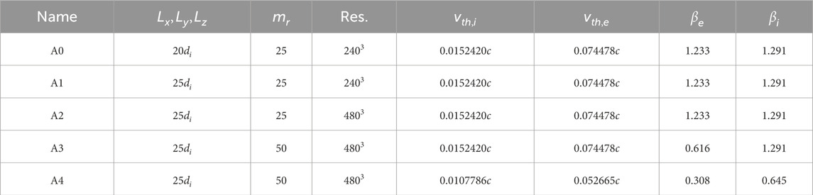
Table 1. Simulation parameters.
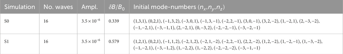
Table 2. List of simulations, the number of wavenumbers in the initial condition, amplitude of waves, initial perturbation amplitude, and the initial mode-numbers.
3 Dispersion and polarization properties
We check the linear dispersion properties of the KAW by comparing the frequency measured in KAW simulations with the frequency calculated from the two-fluid model and frequency from the NHDS (New Hampshire Dispersion Solver) which is a dispersion solver for the fully kinetic case (Verscharen and Chandran, 2018; Verscharen et al., 2013). We take the KAW root of Equation 5 and evaluate it for different values of the wavenumbers. Then simulations are run with single KAW modes corresponding to these wavenumbers. The frequencies from the simulation are obtained by using the magnetic field
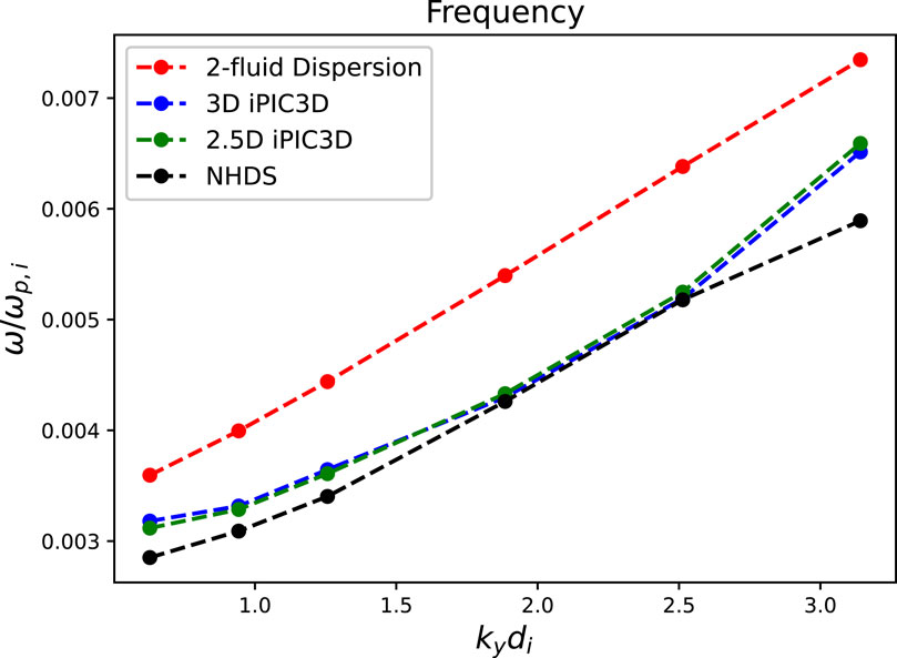
Figure 1. Comparison of frequencies
Figure 1 shows that the observed frequency follows the trend but is smaller than that expected from the two-fluid dispersion relation. This is very similar to the result obtained in Makwana et al. (2023) for similar simulation parameters. It was shown there that the observed dispersion relation matches much better with a hot plasma dispersion relation, even though we use a two-fluid description in the initialization. That showed that such an initialization is suitable for PIC simulations. Here also, we find that the NHDS dispersion relation results are very close to those observed in our 3D simulations. Hence we conclude that the 2-fluid eigenvector is a good initialization for 3D simulation also, while being easier to implement than a fully kinetic initialization. We also checked for the value of
Figure 2 shows the RMS amplitude of the magnetic field perturbations, i.e.,
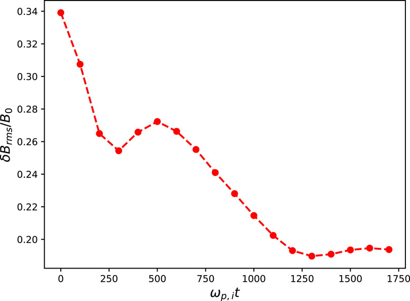
Figure 2.
3.1 Magnetic perturbation ratios
The ratio
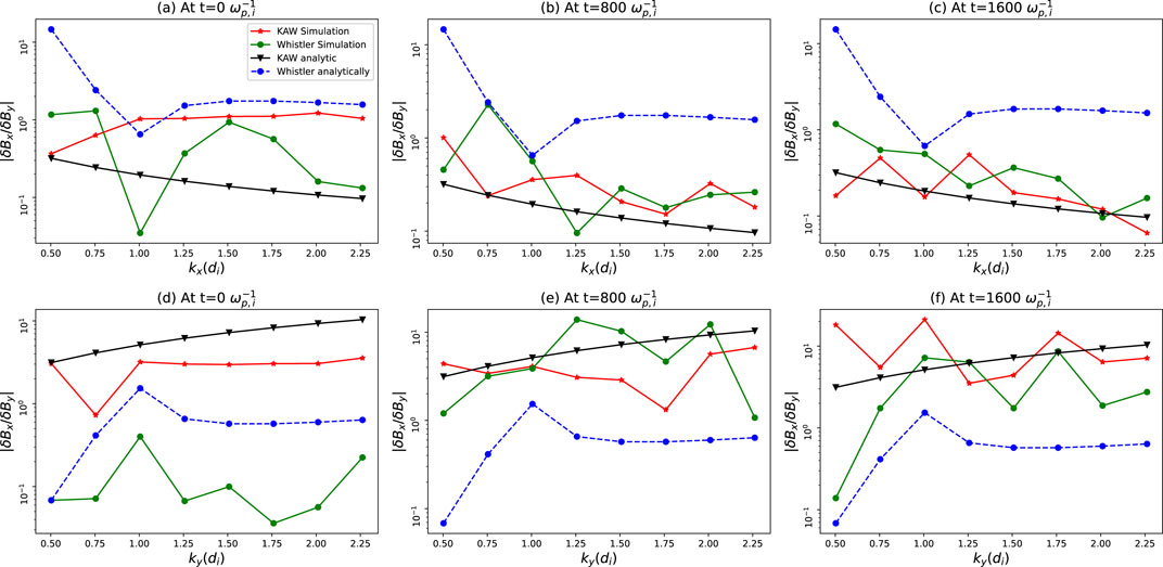
Figure 3.
At
We also look at the ratio
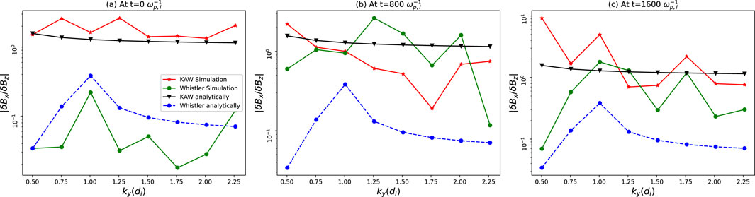
Figure 4.
The ratio
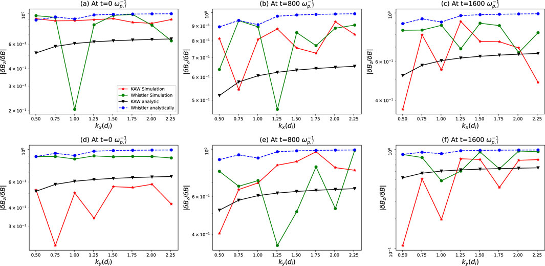
Figure 5.
We have also run these simulations with 125 particles per cell per species, and we get similar results. This indicates that noise is not affecting our results. From the spectra, we can see that noise becomes important at
3.2 Number density perturbation
The ratio of density perturbation to mean number density for ions along
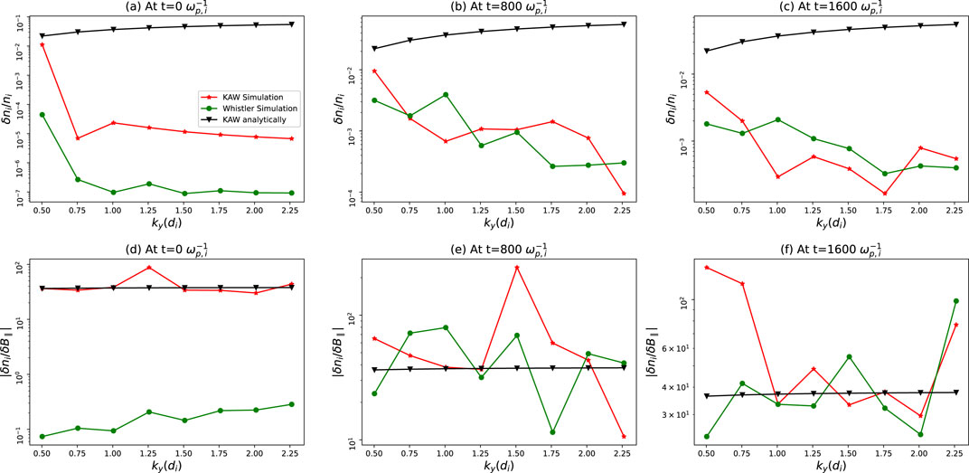
Figure 6. The ratio of ion density perturbation to the mean ion density at time (A)
3.3 Velocity perturbation ratios
We now compare the velocity perturbation ratio
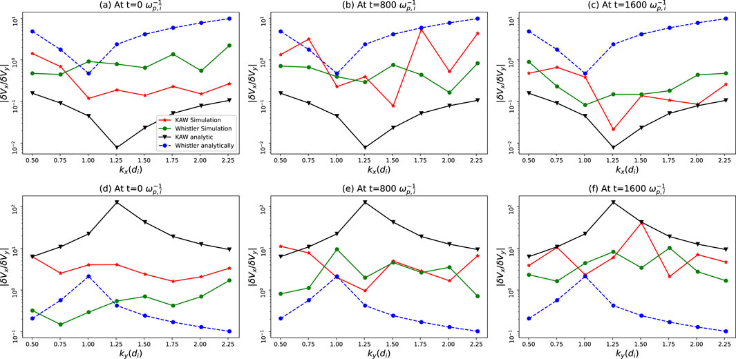
Figure 7. The ratio of velocity perturbation
4 Energy spectrum
4.1 Magnetic energy and velocity spectrum
Now we look at the spectra that are produced by the KAW simulations. We have calculated the magnetic energy and velocity spectrum along the perpendicular wavevector
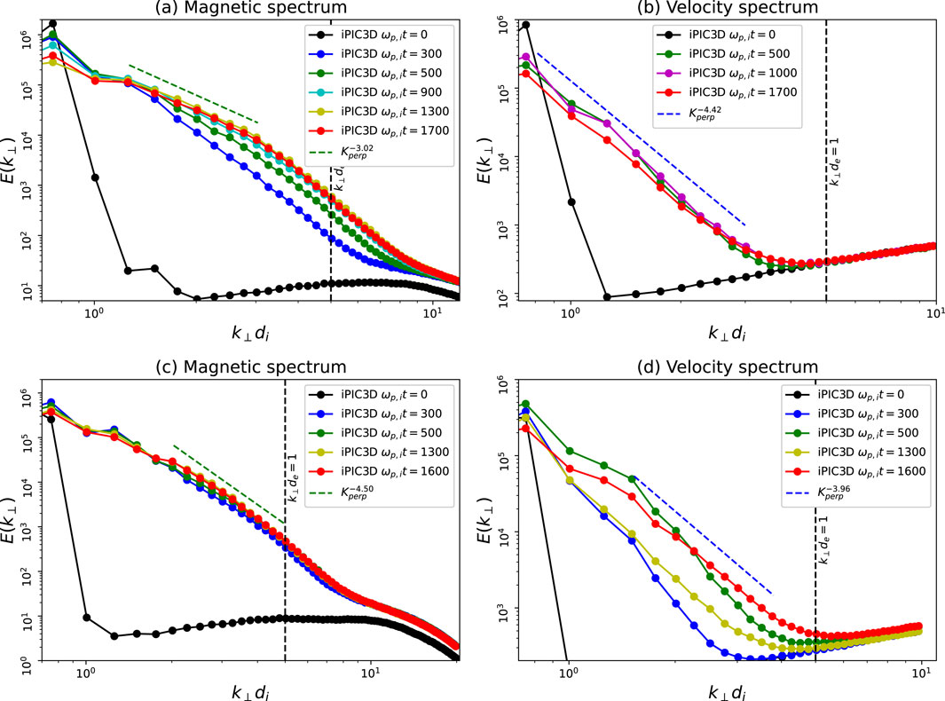
Figure 8. The (A) magnetic energy and (B) velocity spectrum for KAW simulation, and (C) magnetic energy and (D) velocity spectrum for whistler simulation at different times with respect to the perpendicular wavevector
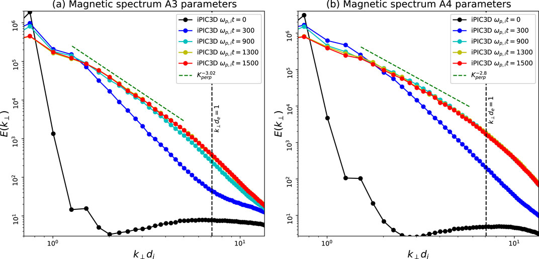
Figure 9. The magnetic energy spectrum
Previously Makwana et al. (2023), we have shown perpendicular magnetic energy spectrum obtained by 2.5D PIC simulations, and the spectrum is similar to 3D case but less smooth and clear. The reason can be given to the fact that in the 3D case, for obtaining the perpendicular spectrum, we have to average over a ring on the perpendicular wavevector plane, while for the 2D case, there is no averaging. Huang et al. (2020) have also obtained the magnetic power spectrum for the solar wind with data taken from NASA’s Parker Solar Probe. They have obtained the power spectrum for both the parallel and the perpendicular direction and have got different slopes. For the perpendicular magnetic spectrum in the transition range (also called the sub-ion range), they have obtained a power law slope of −3.73. There is a large variation in the spectral slope in the sub-ion range (Sahraoui et al., 2009; Sahraoui et al., 2010; Bruno and Trenchi, 2014; Bruno et al., 2014) depending on various physical conditions of the solar wind. The spectral slopes measured in our simulations also lie within this range.
The velocity field spectrum in the perpendicular direction is also obtained and its behaviour is similar to the magnetic spectrum. Initially, at
We have also run KAW simulations with different mass ratios and different ion and electron thermal velocities. The magnetic power spectra in the perpendicular direction for these simulations are shown in Figure 9. Figure 9A shows the magnetic spectrum with a ion-to-electron mass ratio of 50 and A3 parameters. This results in the decrease of electron beta
4.2 2D magnetic energy power spectrum
To understand these interactions in more detail we obtain the 2-dimensional magnetic field power spectrum for KAW simulation in the
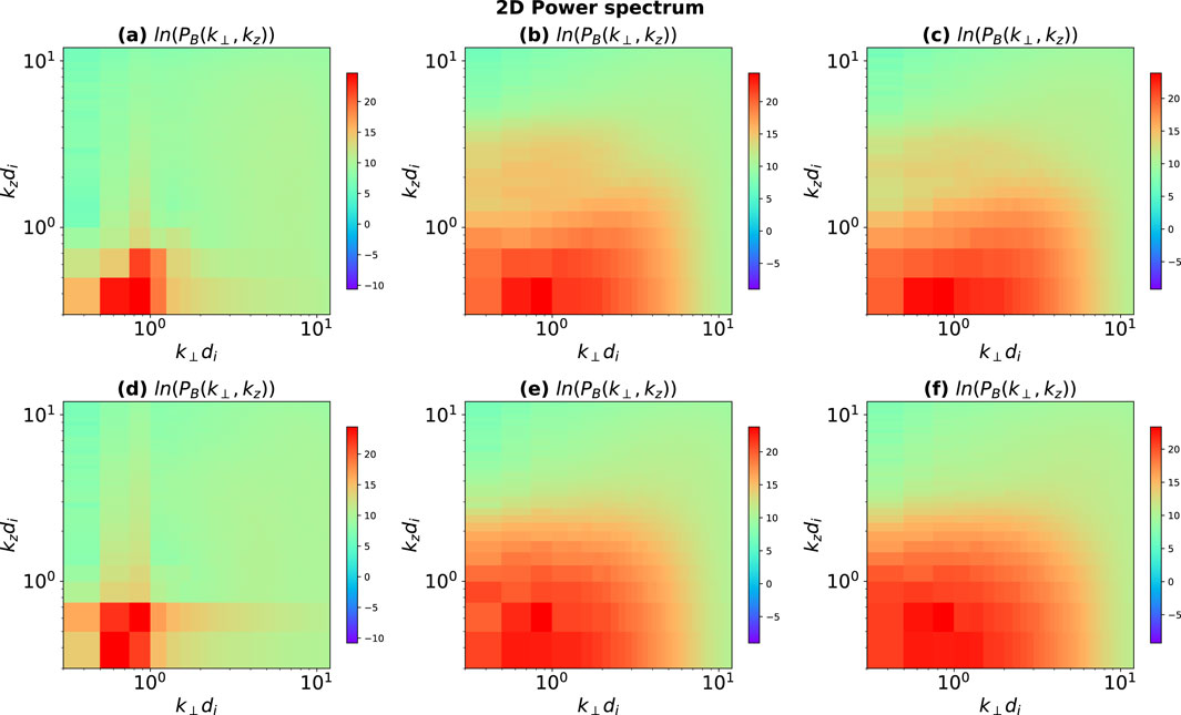
Figure 10. The logarithm of 2 dimensional magnetic energy spectrum
5 Conclusion
In this study, we found that the two-fluid KAW eigenvector relations work well as an initial condition in a fully kinetic 3D PIC simulation. Previously, in Makwana et al. (2023), we did 2.5D PIC simulations and showed that the two-fluid eigenvector relations gave a linear dispersion relation close to the hot plasma kinetic dispersion relation. In this work we extend that study to full 3D PIC simulations. Comparison of the analytical two-fluid KAW dispersion relation, 2.5D simulations, and 3D simulations shows that the frame rotation works appropriately in order to set up initial conditions for different wave-mode simulations.
The simulations are initialized at small wavenumbers (large scales) by either KAWs or whistlers. Therefore, initially, the magnetic perturbation ratios
The perpendicular magnetic energy spectrum obtained for the KAW simulation by running the simulation with
A more detailed picture of the non-linear interactions of KAWs in the simulation is shown by the 2D magnetic energy spectrum in the
There have been earlier studies showing nonlinear generation of whistlers by pump KAWs (Dwivedi et al., 2012) and also excitation of low-frequency KAWs by whistlers (Goyal et al., 2017). There is also the possibility of the co-existence of whistler modes and KAWs (Mithaiwala et al., 2012). However, this generally happens closer to the electron scales. The cascade of whistler waves has also been simulated in PIC at close to the electron scales (Gary et al., 2008). In this study we find that at the sub-ion scales, KAWs are preferentially excited compared to whistlers. It needs to be studied whether it is simply conversion of the Alfvén cascade at magnetohydrodynamic scales into a KAW cascade (Xiang et al., 2019) and/or is it also excitation of the KAWs by some instabilities. One drawback of this study is that it simulates decaying turbulence. More general forced simulations will provide better characteristics of turbulence. Also, there could be other modes playing an important role in addition to the two modes studied here. To study further smaller scales, we would need to use kinetic dispersion properties. Furthermore, the resolution is quite limited. We require higher resolution in both space and time, with higher mass ratios, to obtain more realistic kinetic range turbulence properties.
Data availability statement
The raw data supporting the conclusions of this article will be made available by the authors, without undue reservation.
Author contributions
JS: Data curation, Formal Analysis, Investigation, Methodology, Project administration, Software, Validation, Visualization, Writing–original draft, Writing–review and editing. KM: Conceptualization, Funding acquisition, Investigation, Supervision, Validation, Writing–review and editing, Methodology, Resources, Formal Analysis, Writing–original draft.
Funding
The author(s) declare that financial support was received for the research, authorship, and/or publication of this article. This work was supported by Science and Engineering Research Board (SERB) grant SRG/2021/001439. We would like to thank DST – FIST (SR/FST/PSI-215/2016) for the financial support alongwith Indian Institute of Technology, Hyderabad seed grant. The support and the resources provided by the “PARAM Sanganak facility” under the National Supercomputing Mission, Government of India at the Indian Institute of Technology, Kanpur, as well as the “PARAM Seva facility” at Indian Institute of Technology, Hyderabad are gratefully acknowledged.
Acknowledgments
KM acknowledges useful discussions with Dr. M. K. Verma.
Conflict of interest
The authors declare that the research was conducted in the absence of any commercial or financial relationships that could be construed as a potential conflict of interest.
Publisher’s note
All claims expressed in this article are solely those of the authors and do not necessarily represent those of their affiliated organizations, or those of the publisher, the editors and the reviewers. Any product that may be evaluated in this article, or claim that may be made by its manufacturer, is not guaranteed or endorsed by the publisher.
Supplementary material
The Supplementary Material for this article can be found online at: https://www.frontiersin.org/articles/10.3389/fspas.2024.1423642/full#supplementary-material
References
AC-L, C. (1995). Nonlinear alfvén wave phenomena in the planetary magnetosphere. doi:10.1088/0031-8949/1995/T60/005
Alexandrova, O., Chen, C. H., Sorriso-Valvo, L., Horbury, T. S., and Bale, S. D. (2013). Solar wind turbulence and the role of ion instabilities. Space Sci. Rev. 178, 101–139. doi:10.1007/s11214-013-0004-8
Alexandrova, O., Saur, J., Lacombe, C., Mangeney, A., Mitchell, J., Schwartz, S. J., et al. (2009). Universality of solar-wind turbulent spectrum from mhd to electron scales. Phys. Rev. Lett. 103, 165003. doi:10.1103/PhysRevLett.103.165003
Alfvén, H. (1942). Existence of electromagnetic-hydrodynamic waves. Nature 150, 405–406. doi:10.1038/150405d0
Arzamasskiy, L., Kunz, M. W., Chandran, B. D., and Quataert, E. (2019). Hybrid-kinetic simulations of ion heating in alfvénic turbulence. Astrophysical J. 879, 53. doi:10.3847/1538-4357/ab20cc
Bamert, K., Kallenbach, R., le Roux, J. A., Hilchenbach, M., Smith, C. W., and Wurz, P. (2008). Evidence for iroshnikov-kraichnan-type turbulence in the solar wind upstream of interplanetary traveling shocks. Astrophysical J. 675, L45–L48. doi:10.1086/529491
Belcher, J. W., and Davis, L. J. (1971). Large-amplitude alfvén waves in the interplanetary medium, 2. J. Geophys. Res. Space Phys. 76, 3534–3563. doi:10.1029/ja076i016p03534
Bhattacharjee, A., and Ng, C. (2001). Random scattering and anisotropic turbulence of shear alfvén wave packets. Astrophysical J. 548, 318–322. doi:10.1086/318692
Boldyrev, S. (2006). Spectrum of magnetohydrodynamic turbulence. Phys. Rev. Lett. 96, 115002. doi:10.1103/PhysRevLett.96.115002
Boldyrev, S., Horaites, K., Xia, Q., and Perez, J. C. (2013). Toward a theory of astrophysical plasma turbulence at subproton scales. Astrophysical J. 777, 41. doi:10.1088/0004-637X/777/1/41
Boldyrev, S., and Perez, J. C. (2012). Spectrum of kinetic-alfvén turbulence. Astrophysical J. Lett. 758, L44. doi:10.1088/2041-8205/758/2/L44
Bowen, T. A., Bale, S. D., Chandran, B. D., Chasapis, A., Chen, C. H., Dudok de Wit, T., et al. (2024). Mediation of collisionless turbulent dissipation through cyclotron resonance. Nat. Astron. 8, 482–490. doi:10.1038/s41550-023-02186-4
Bruno, R., and Carbone, V. (2013). The solar wind as a turbulence laboratory. Living Rev. Sol. Phys. 10, 2. doi:10.12942/lrsp-2013-2
Bruno, R., and Telloni, D. (2015). Spectral analysis of magnetic fluctuations at proton scales from fast to slow solar wind. Astrophysical J. Lett. 811, L17. doi:10.1088/2041-8205/811/2/L17
Bruno, R., and Trenchi, L. (2014). Radial dependence of the frequency break between fluid and kinetic scales in the solar wind fluctuations. Astrophysical J. Lett. 787, L24. doi:10.1088/2041-8205/787/2/L24
Bruno, R., Trenchi, L., and Telloni, D. (2014). Spectral slope variation at proton scales from fast to slow solar wind. Astrophysical J. Lett. 793, L15. doi:10.1088/2041-8205/793/1/L15
Califano, F., Cerri, S. S., Faganello, M., Laveder, D., Sisti, M., and Kunz, M. W. (2020). Electron-only reconnection in plasma turbulence. Front. Phys. 8, 317. doi:10.3389/fphy.2020.00317
Camporeale, E., and Burgess, D. (2011). The dissipation of solar wind turbulent fluctuations at electron scales. Astrophys. J. 730, 114. doi:10.1088/0004-637X/730/2/114
Cerri, S., Kunz, M. W., and Califano, F. (2018). Dual phase-space cascades in 3d hybrid-vlasov–maxwell turbulence. Astrophysical J. Lett. 856, L13. doi:10.3847/2041-8213/aab557
Cerri, S. S., Arzamasskiy, L., and Kunz, M. W. (2021). On stochastic heating and its phase-space signatures in low-beta kinetic turbulence. Astrophysical J. 916, 120. doi:10.3847/1538-4357/abfbde
Cerri, S. S., and Califano, F. (2017). Reconnection and small-scale fields in 2d-3v hybrid-kinetic driven turbulence simulations. New J. Phys. 19, 025007. doi:10.1088/1367-2630/aa5c4a
Cerri, S. S., Califano, F., Jenko, F., Told, D., and Rincon, F. (2016). Subproton-scale cascades in solar wind turbulence: driven hybrid-kinetic simulations. Astrophysical J. Lett. 822, L12. doi:10.3847/2041-8205/822/1/L12
Cerri, S. S., Franci, L., Califano, F., Landi, S., and Hellinger, P. (2017). Plasma turbulence at ion scales: a comparison between particle in cell and eulerian hybrid-kinetic approaches. J. Plasma Phys. 83, 705830202. doi:10.1017/S0022377817000265
Cerri, S. S., Grošelj, D., and Franci, L. (2019). Kinetic plasma turbulence: recent insights and open questions from 3d3v simulations. Front. Astronomy Space Sci. 6, 64. doi:10.3389/fspas.2019.00064
Chang, O., Gary, S. P., and Wang, J. (2015). Whistler turbulence forward vs. inverse cascade. three-dimensional particle-in-cell simulations. Astrophysical J. (Online) 800, 87. doi:10.1088/0004-637X/800/2/87
Chang, O., Peter Gary, S., and Wang, J. (2011). Whistler turbulence forward cascade: three-dimensional particle-in-cell simulations. Geophys. Res. Lett. 38. doi:10.1029/2011GL049827
Chen, C. (2016). Recent progress in astrophysical plasma turbulence from solar wind observations. J. Plasma Phys. 82, 535820602. doi:10.1017/S0022377816001124
Chen, C., Boldyrev, S., Xia, Q., and Perez, J. (2013). Nature of subproton scale turbulence in the solar wind. Phys. Rev. Lett. 110, 225002. doi:10.1103/PhysRevLett.110.225002
Chen, C. H. K., and Boldyrev, S. (2017). Nature of kinetic scale turbulence in the earth's magnetosheath. Astrophys. J. 842, 122. doi:10.3847/1538-4357/aa74e0
Cho, J., and Vishniac, E. T. (2000). The anisotropy of magnetohydrodynamic alfvénic turbulence. Astrophys. J. 539, 273–282. doi:10.1086/309213
Coleman, J. (1968). Turbulence, viscosity, and dissipation in the solar-wind plasma. Astrophys. J. 153, 371. doi:10.1086/149674
David, V., and Galtier, S. (2019). Spectrum in kinetic alfvén wave turbulence: implications for the solar wind. Astrophysical J. Lett. 880, L10. doi:10.3847/2041-8213/ab2fe6
Dwivedi, N. K., Batra, K., and Sharma, R. P. (2012). Study of kinetic Alfvén wave and whistler wave spectra and their implication in solar wind plasma. J. Geophys. Res. (Space Phys.) 117, A07201. doi:10.1029/2011JA017234
Franci, L., Cerri, S. S., Califano, F., Landi, S., Papini, E., Verdini, A., et al. (2017). Magnetic reconnection as a driver for a sub-ion-scale cascade in plasma turbulence. Astrophysical J. Lett. 850, L16. doi:10.3847/2041-8213/aa93fb
Franci, L., Landi, S., Matteini, L., Verdini, A., and Hellinger, P. (2015). High-resolution hybrid simulations of kinetic plasma turbulence at proton scales. Astrophysical J. 812, 21. doi:10.1088/0004-637X/812/1/21
Franci, L., Landi, S., Matteini, L., Verdini, A., and Hellinger, P. (2016). Plasma beta dependence of the ion-scale spectral break of solar wind turbulence: high-resolution 2d hybrid simulations. Astrophysical J. 833, 91. doi:10.3847/1538-4357/833/1/91
Franci, L., Landi, S., Verdini, A., Matteini, L., and Hellinger, P. (2018). Solar wind turbulent cascade from mhd to sub-ion scales: large-size 3d hybrid particle-in-cell simulations. Astrophysical J. 853, 26. doi:10.3847/1538-4357/aaa3e8
Franci, L., Papini, E., Micera, A., Lapenta, G., Hellinger, P., Del Sarto, D., et al. (2022). Anisotropic electron heating in turbulence-driven magnetic reconnection in the near-sun solar wind. Astrophysical J. 936, 27. doi:10.3847/1538-4357/ac7da6
Friedrich, J., Wilbert, M., and Marino, R. (2024). Nonlocal contributions to the turbulent cascade in magnetohydrodynamic plasmas. Phys. Rev. E 109, 045208. doi:10.1103/PhysRevE.109.045208
Galtier, S., Nazarenko, S., Newell, A. C., and Pouquet, A. (2000). A weak turbulence theory for incompressible magnetohydrodynamics. J. plasma Phys. 63, 447–488. doi:10.1017/S0022377899008284
Gary, S. P., Bandyopadhyay, R., Qudsi, R. A., Matthaeus, W. H., Maruca, B. A., Parashar, T. N., et al. (2020). Particle-in-cell simulations of decaying plasma turbulence: linear instabilities versus nonlinear processes in 3d and 2.5 d approximations. Astrophysical J. 901, 160. doi:10.3847/1538-4357/abb2ac
Gary, S. P., Chang, O., and Wang, J. (2012). Forward cascade of whistler turbulence: three-dimensional particle-in-cell simulations. Astrophysical J. 755, 142. doi:10.1088/0004-637X/755/2/142
Gary, S. P., Saito, S., and Li, H. (2008). Cascade of whistler turbulence: particle-in-cell simulations. Geophys. Res. Lett. 35. doi:10.1029/2007GL032327
Gary, S. P., and Smith, C. W. (2009). Short-wavelength turbulence in the solar wind: linear theory of whistler and kinetic alfvén fluctuations. J. Geophys. Res. Space Phys. 114. doi:10.1029/2009JA014525
Goldreich, P., and Sridhar, S. (1995). Toward a theory of interstellar turbulence. 2: strong alfvenic turbulence. Astrophysical J. Part 1 438 (2), 763–775. ISSN 0004-637X. doi:10.1086/175121
Gorman, W., and Klein, K. G. (2024). Mind the gap: non-local cascades and preferential heating in high-β Alfvénic turbulence. Mon. Notices R. Astronomical Soc. Lett. 531, L1–L7. doi:10.1093/mnrasl/slae018
Goyal, R., Sharma, R. P., and Kumar, S. (2017). Nonlinear effects associated with quasi-electrostatic whistler waves relevant to that in radiation belts. J. Geophys. Res. (Space Phys.) 122, 340–348. doi:10.1002/2016JA023274
Grošelj, D., Cerri, S. S., Navarro, A. B., Willmott, C., Told, D., Loureiro, N. F., et al. (2017). Fully kinetic versus reduced-kinetic modeling of collisionless plasma turbulence. Astrophysical J. 847, 28. doi:10.3847/1538-4357/aa894d
Grošelj, D., Chen, C. H., Mallet, A., Samtaney, R., Schneider, K., and Jenko, F. (2019). Kinetic turbulence in astrophysical plasmas: waves and/or structures? Phys. Rev. X 9, 031037. doi:10.1103/PhysRevX.9.031037
Grošelj, D., Mallet, A., Loureiro, N. F., and Jenko, F. (2018). Fully kinetic simulation of 3d kinetic alfvén turbulence. Phys. Rev. Lett. 120, 105101. doi:10.1103/PhysRevLett.120.105101
Hasegawa, A., and Chen, L. (1976). Kinetic processes in plasma heating by resonant mode conversion of Alfvén wave. Princeton, NJ (United States): Princeton Plasma Physics Lab, PPPL. Tech. Rep. doi:10.1063/1.861427
Hasegawa, A., and Uberoi, C. (1982). The alfvén wave. DOE Crit. Rev. Ser. DOE/TIC–11197. doi:10.2172/5259641
Hollweg, J. V. (1999). Kinetic alfvén wave revisited. J. Geophys. Res. Space Phys. 104, 14811–14819. doi:10.1029/1998JA900132
Howes, G. G., Cowley, S. C., Dorland, W., Hammett, G. W., Quataert, E., and Schekochihin, A. A. (2008). A model of turbulence in magnetized plasmas: implications for the dissipation range in the solar wind. J. Geophys. Res. Space Phys. 113. doi:10.1029/2007JA012665
Howes, G. G., TenBarge, J. M., Dorland, W., Quataert, E., Schekochihin, A. A., Numata, R., et al. (2011). Gyrokinetic simulations of solar wind turbulence from ion to electron scales. Phys. Rev. Lett. 107, 035004. doi:10.1103/PhysRevLett.107.035004
Huang, S., Sahraoui, F., Andrés, N., Hadid, L., Yuan, Z., He, J., et al. (2021). The ion transition range of solar wind turbulence in the inner heliosphere: Parker solar probe observations. Astrophysical J. Lett. 909, L7. doi:10.3847/2041-8213/abdaaf
Huang, S., Zhang, J., Sahraoui, F., He, J., Yuan, Z., Andrés, N., et al. (2020). Kinetic scale slow solar wind turbulence in the inner heliosphere: Co-existence of kinetic alfvén waves and alfvén ion cyclotron waves. Astrophysical J. Lett. 897, L3. doi:10.3847/2041-8213/ab9abb
Iroshnikov, P. S. (1963). Turbulence of a conducting fluid in a strong magnetic field. Astron. Zhurnal 40, 742.
Kiyani, K. H., Chapman, S. C., Sahraoui, F., Hnat, B., Fauvarque, O., and Khotyaintsev, Y. V. (2013). Enhanced magnetic compressibility and isotropic scale invariance at sub-ion larmor scales in solar wind turbulence. Astrophysical J. 763, 10. doi:10.1088/0004-637X/763/1/10
Kobayashi, S., Sahraoui, F., Passot, T., Laveder, D., Sulem, P., Huang, S., et al. (2017). Three-dimensional simulations and spacecraft observations of sub-ion scale turbulence in the solar wind: influence of landau damping. Astrophysical J. 839, 122. doi:10.3847/1538-4357/aa67f2
Kolmogorov, A. (1941). The local structure of turbulence in incompressible viscous fluid for very large Reynolds’ numbers. Akad. Nauk. SSSR Dokl. 30, 301–305.
Kraichnan, R. H. (1965). Inertial-range spectrum of hydromagnetic turbulence. Phys. Fluids 8, 1385–1387. doi:10.1063/1.1761412
Lapenta, G. (2012). Particle simulations of space weather. J. Comput. Phys. 231, 795–821. doi:10.1016/j.jcp.2011.03.035
Makwana, K., Bhagvati, S., and Sharma, J. (2023). Linear dispersion and nonlinear interactions in 2.5 d particle-in-cell simulations of kinetic alfvén waves. Plasma Phys. Rep. 49, 759–771. doi:10.1134/S1063780X2260133X
Makwana, K. D., and Yan, H. (2020). Properties of magnetohydrodynamic modes in compressively driven plasma turbulence. Phys. Rev. X 10, 031021. doi:10.1103/PhysRevX.10.031021
Markidis, S., Lapenta, G., and Rizwan-uddin, (2010). Multi-scale simulations of plasma with ipic3d. Math. Comput. Simul. 80, 1509–1519. doi:10.1016/j.matcom.2009.08.038
Matteini, L., Alexandrova, O., Chen, C., and Lacombe, C. (2017). Electric and magnetic spectra from mhd to electron scales in the magnetosheath. Mon. Notices R. Astronomical Soc. 466, 945–951. doi:10.1093/mnras/stw3163
Matteini, L., Franci, L., Alexandrova, O., Lacombe, C., Landi, S., Hellinger, P., et al. (2020). Magnetic field turbulence in the solar wind at sub-ion scales: in situ observations and numerical simulations. Front. Astronomy Space Sci. 7, 563075. doi:10.3389/fspas.2020.563075
Matthaeus, W. H., Goldstein, M. L., and Montgomery, D. C. (1983). Turbulent generation of outward-traveling interplanetary alfvénic fluctuations. Phys. Rev. Lett. 51, 1484–1487. doi:10.1103/PhysRevLett.51.1484
Matthaeus, W. H., Yang, Y., Wan, M., Parashar, T. N., Bandyopadhyay, R., Chasapis, A., et al. (2020). Pathways to dissipation in weakly collisional plasmas. Astrophysical J. 891, 101. doi:10.3847/1538-4357/ab6d6a
Meyrand, R., Squire, J., Schekochihin, A. A., and Dorland, W. (2021). On the violation of the zeroth law of turbulence in space plasmas. J. Plasma Phys. 87, 535870301. doi:10.1017/S0022377821000489
Mithaiwala, M., Rudakov, L., Crabtree, C., and Ganguli, G. (2012). Co-existence of whistler waves with kinetic Alfven wave turbulence for the high-beta solar wind plasma. Phys. Plasmas 19, 102902. doi:10.1063/1.4757638
Muñoz, P. A., Jain, N., Farzalipour Tabriz, M., Rampp, M., and Büchner, J. (2023). Electron inertia effects in 3d hybrid-kinetic collisionless plasma turbulence. Phys. Plasmas 30. doi:10.1063/5.0148818
Narita, Y., Roberts, O. W., Vörös, Z., and Hoshino, M. (2020). Transport ratios of the kinetic alfvén mode in space plasmas. Front. Phys. 8, 166. doi:10.3389/fphy.2020.00166
Ofman, L. (2010). Wave modeling of the solar wind. Living Rev. Sol. Phys. 7, 4–48. doi:10.12942/lrsp-2010-4
Olshevsky, V., Servidio, S., Pucci, F., Primavera, L., and Lapenta, G. (2018). Properties of decaying plasma turbulence at subproton scales. Astrophysical J. 860, 11. doi:10.3847/1538-4357/aac1bd
Parashar, T., Servidio, S., Breech, B., Shay, M., and Matthaeus, W. (2010). Kinetic driven turbulence: structure in space and time. Phys. Plasmas 17. doi:10.1063/1.3486537
Parashar, T., Servidio, S., Shay, M., Breech, B., and Matthaeus, W. (2011). Effect of driving frequency on excitation of turbulence in a kinetic plasma. Phys. Plasmas 18. doi:10.1063/1.3630926
Parashar, T. N., Matthaeus, W. H., and Shay, M. A. (2018). Dependence of kinetic plasma turbulence on plasma dependence of kinetic plasma turbulence on plasma β. Astrophysical J. Lett. 864, L21. doi:10.3847/2041-8213/aadb8b
Passot, T., Cerri, S., Granier, C., Laveder, D., Sulem, P., and Tassi, E. (2024). Gyrofluid simulations of turbulence and reconnection in space plasmas. Fundam. Plasma Phys. 11, 100055. doi:10.1016/j.fpp.2024.100055
Passot, T., and Sulem, P. (2019). Imbalanced kinetic alfvén wave turbulence: from weak turbulence theory to nonlinear diffusion models for the strong regime. J. Plasma Phys. 85, 905850301. doi:10.1017/S0022377819000187
Passot, T., Sulem, P., and Laveder, D. (2022). Direct kinetic alfvén wave energy cascade in the presence of imbalance. J. Plasma Phys. 88, 905880312. doi:10.1017/S0022377822000472
Perrone, D., Passot, T., Laveder, D., Valentini, F., Sulem, P., Zouganelis, I., et al. (2018). Fluid simulations of plasma turbulence at ion scales: comparison with vlasov-maxwell simulations. Phys. Plasmas 25. doi:10.1063/1.5026656
Pezzi, O., Parashar, T., Servidio, S., Valentini, F., Vásconez, C., Yang, Y., et al. (2017). Colliding Alfvénic wave packets in magnetohydrodynamics, Hall and kinetic simulations. J. plasma Phys. 83, 705830108. doi:10.1017/S0022377817000113
Pezzi, O., Servidio, S., Perrone, D., Valentini, F., Sorriso-Valvo, L., Greco, A., et al. (2018). Velocity-space cascade in magnetized plasmas: numerical simulations. Phys. Plasmas 25. doi:10.1063/1.5027685
Podesta, J. J., Roberts, D. A., and Goldstein, M. L. (2007). Spectral exponents of kinetic and magnetic energy spectra in solar wind turbulence. Astrophys. J. 664, 543–548. doi:10.1086/519211
Roberts, D. A. (2007). “The evolution of the spectrum of velocity fluctuations in the solar wind,” in AGU Fall Meeting Abstracts. SH31B–06.2007
Sahraoui, F., Goldstein, M., Robert, P., and Khotyaintsev, Y. V. (2009). Evidence of a cascade and dissipation of solar-wind turbulence at the electron gyroscale. Phys. Rev. Lett. 102, 231102. doi:10.1103/PhysRevLett.102.231102
Sahraoui, F., Goldstein, M. L., Belmont, G., Canu, P., and Rezeau, L. (2010). Three dimensional anisotropic k spectra of turbulence at subproton scales in the solar wind. Phys. Rev. Lett. 105, 131101. doi:10.1103/PhysRevLett.105.131101
Sahraoui, F., Huang, S., Belmont, G., Goldstein, M., Retinò, A., Robert, P., et al. (2013). Scaling of the electron dissipation range of solar wind turbulence. Astrophysical J. 777, 15. doi:10.1088/0004-637X/777/1/15
Saito, S., and Peter Gary, S. (2012). Beta dependence of electron heating in decaying whistler turbulence: particle-in-cell simulations. Phys. Plasmas 19, 012312. doi:10.1063/1.3676155
Salem, C. S., Howes, G., Sundkvist, D., Bale, S., Chaston, C., Chen, C., et al. (2012). Identification of kinetic alfvén wave turbulence in the solar wind. Astrophysical J. Lett. 745, L9. doi:10.1088/2041-8205/745/1/L9
Schekochihin, A., Cowley, S. C., Dorland, W., Hammett, G., Howes, G. G., Quataert, E., et al. (2009). Astrophysical gyrokinetics: kinetic and fluid turbulent cascades in magnetized weakly collisional plasmas. Astrophysical J. Suppl. Ser. 182, 310–377. doi:10.1088/0067-0049/182/1/310
Schekochihin, A. A. (2022). Mhd turbulence: a biased review. J. Plasma Phys. 88, 155880501. doi:10.1017/S0022377822000721
Servidio, S., Valentini, F., Perrone, D., Greco, A., Califano, F., Matthaeus, W., et al. (2015). A kinetic model of plasma turbulence. J. Plasma Phys. 81, 325810107. doi:10.1017/S0022377814000841
Shaikh, D., and Zank, G. (2009). Spectral features of solar wind turbulent plasma. Mon. notices R. astronomical Soc. 400, 1881–1891. doi:10.1111/j.1365-2966.2009.15579.x
Sharma, R., Rozmus, W., and Offenberger, A. (1986). Stimulated brillouin scattering of whistler waves off the kinetic alfvén waves in plasmas. Phys. fluids 29, 4055–4059. doi:10.1063/1.865748
Shebalin, J. V., Matthaeus, W. H., and Montgomery, D. (1983). Anisotropy in MHD turbulence due to a mean magnetic field. J. Plasma Phys. 29, 525–547. doi:10.1017/S0022377800000933
Sisti, M., Fadanelli, S., Cerri, S. S., Faganello, M., Califano, F., and Agullo, O. (2021). Characterizing current structures in 3d hybrid-kinetic simulations of plasma turbulence. Astronomy and Astrophysics 655, A107. doi:10.1051/0004-6361/202141902
Squire, J., Meyrand, R., Kunz, M. W., Arzamasskiy, L., Schekochihin, A. A., and Quataert, E. (2022). High-frequency heating of the solar wind triggered by low-frequency turbulence. Nat. Astron. 6, 715–723. doi:10.1038/s41550-022-01624-z
TenBarge, J., Howes, G., and Dorland, W. (2013). Collisionless damping at electron scales in solar wind turbulence. Astrophysical J. 774, 139. doi:10.1088/0004-637X/774/2/139
TenBarge, J., Podesta, J., Klein, K., and Howes, G. (2012). Interpreting magnetic variance anisotropy measurements in the solar wind. Astrophysical J. 753, 107. doi:10.1088/0004-637X/753/2/107
Told, D., Jenko, F., TenBarge, J. M., Howes, G. G., and Hammett, G. W. (2015). Multiscale nature of the dissipation range in gyrokinetic simulations of alfvénic turbulence. Phys. Rev. Lett. 115, 025003. doi:10.1103/PhysRevLett.115.025003
Valentini, F., Servidio, S., Perrone, D., Califano, F., Matthaeus, W., and Veltri, P. (2014). Hybrid vlasov-maxwell simulations of two-dimensional turbulence in plasmas. Phys. Plasmas 21. doi:10.1063/1.4893301
Vásconez, C., Pucci, F., Valentini, F., Servidio, S., Matthaeus, W., and Malara, F. (2015). Kinetic alfvén wave generation by large-scale phase mixing. Astrophysical J. 815, 7. doi:10.1088/0004-637X/815/1/7
Verscharen, D., Bourouaine, S., Chandran, B. D., and Maruca, B. A. (2013). A parallel-propagating alfvénic ion-beam instability in the high-beta solar wind. Astrophysical J. 773, 8. doi:10.1088/0004-637X/773/1/8
Verscharen, D., and Chandran, B. D. (2018). Nhds: the New Hampshire dispersion relation solver. Res. Notes AAS 2, 13. doi:10.3847/2515-5172/aabfe3
Verscharen, D., Klein, K. G., and Maruca, B. A. (2019). The multi-scale nature of the solar wind. Living Rev. Sol. Phys. 16, 5. doi:10.1007/s41116-019-0021-0
Voitenko, Y., and De Keyser, J. (2011). Turbulent spectra and spectral kinks in the transition range from mhd to kinetic alfvén turbulence. Nonlinear Process. Geophys. 18, 587–597. doi:10.5194/npg-18-587-2011
Voitenko, Y., and De Keyser, J. (2016). Mhd-kinetic transition in imbalanced alfvénic turbulence. Astrophysical J. Lett. 832, L20. doi:10.3847/2041-8205/832/2/L20
Voitenko, Y., and Goossens, M. (2004). Excitation of kinetic alfvén turbulence by mhd waves and energization of space plasmas. Nonlinear Process. Geophys. 11, 535–543. doi:10.5194/npg-11-535-2004
Voitenko, Y., and Goossens, M. (2006). Energization of plasma species by intermittent kinetic alfvén waves. Space Sci. Rev. 122, 255–270. doi:10.1007/s11214-006-8212-0
Keywords: plasma turbulence, kinetic Alfvén waves, PIC simulations, sub-ion scales, solar wind
Citation: Sharma J and Makwana KD (2024) Kinetic Alfvén wave cascade in sub-ion range plasma turbulence. Front. Astron. Space Sci. 11:1423642. doi: 10.3389/fspas.2024.1423642
Received: 26 April 2024; Accepted: 09 October 2024;
Published: 29 October 2024.
Edited by:
Oreste Pezzi, Institute for Plasma Science and Technology (ISTP/CNR), ItalyReviewed by:
Silvio Sergio Cerri, UMR7293 Laboratoire J L Lagrange (LAGRANGE), FranceSubash Adhikari, West Virginia University, United States
Copyright © 2024 Sharma and Makwana. This is an open-access article distributed under the terms of the Creative Commons Attribution License (CC BY). The use, distribution or reproduction in other forums is permitted, provided the original author(s) and the copyright owner(s) are credited and that the original publication in this journal is cited, in accordance with accepted academic practice. No use, distribution or reproduction is permitted which does not comply with these terms.
*Correspondence: Johan Sharma, a2RtYWt3YW5hQHBoeS5paXRoLmFjLmlu