The case for a rectangular format space telescope for finding exoplanets

We suggest that rectangular primary-mirror telescopes provide a clearer path to discovering habitable worlds than other designs currently being pursued. We show that a simple infrared ($\lambda \sim$10 $\mu$m) telescope design with a rectangular mirror 20 m in length and 1 m in width, combined with technology already developed for JWST, can discover $\sim$11 habitable exoplanets and measure ozone in their atmospheres in a mission of $\sim$1 year. A mission of $\sim$3.5 years could plausibly discover $\sim$27 habitable exoplanets closer than 10 pc to the Earth, and determine whether there is ozone in their atmospheres. A square primary mirror with the same collecting area cannot resolve exoplanets that are within 0.23″ of the host star, making it impossible to detect most of the nearby Earth-like exoplanets. The idea of collecting light with a high aspect ratio rectangular mirror could be used at any wavelength. It is particularly useful for measuring point sources with very small angular separations, as is required for exoplanet observation.

1 Introduction

One of the most exciting scientific endeavors of this century is the quest to find a habitable, Earth-like exoplanet. It would be most exciting to find a habitable exoplanet that is close enough to the Earth that one could imagine sending a probe to explore it, or maybe one day sending human explorers. Even more exciting would be the discovery of a planet that has oxygen in its atmosphere, which would make it potentially habitable for us and also likely to support life of its own. Direct imaging of at least 25 habitable exoplanets and finding biosignatures such as oxygen and methane in their atmospheres is in fact the primary science driver for the Habitable Worlds Observatory (HWO), a conceptual future NASA flagship mission that is thought to require a significant technology maturation process (National Academies of Sciences, Engineering, and Medicine, 2021) before it can be selected.

Most current and planned exoplanet discovery missions use the transit method, which relies on the small decrease in starlight observed when an exoplanet passes in front of a star, to find exoplanets. TESS (Ricker et al., 2014) is the current NASA transit mission, following the highly successful Kepler mission (Borucki et al., 2003), which discovered 2,806 of the 5,638 currently known exoplanets according to the NASA Exoplanet Archive (Akeson et al., 2013; NASA Exoplanet Archive, 2024). Both ESA (PLATO, Rauer et al., 2014) and China (Earth 2.0, Ye, 2022) are building new missions to detect Earth-like planets using the transit method and aim to launch in 2026 and 2027 (Zang et al., 2024), respectively. However, only a small fraction of exoplanet orbits are edge-on as observed from the Solar System, so a large volume of the local Galactic neighborhood must be searched to have a high probability of finding an Earth-like planet.

Instruments such as ESPRESSO (Pepe et al., 2021), EXPRES (Jurgenson et al., 2016), and NEID (Schwab et al., 2016) could reach a radial velocity precision of 10 cm/s (compare with the Sun’s speed of 9 cm/s around the Earth-Sun center of mass), if difficulties with velocity variation of the material on the surface of the host star can be overcome. This raises the possibility that habitable exoplanets with a wider range of orbital inclinations could be identified. Even so, the radial velocity method misses planets that orbit face-on.

The only way to find all of the local Earth-like exoplanets is to resolve exoplanets from their host stars, for example, by direct imaging. Resolving exoplanets from their host stars also vastly improves the signal-to-noise for spectroscopy of exoplanet atmospheres. However, to detect Earth, which is 1 AU from the Sun, from a distance of 10 pc requires an angular resolution of 0.1 arcseconds (0.1″). The Sun is more than ten billion times brighter than the Earth in visible (reflected) light, but the luminosity contrast can be reduced by observing in the infrared (optimally $\sim$10 $\mu$m) where the Earth peaks in emission and the Sun is only a million times brighter than the Earth. To separate two objects that are 0.1″ apart at a wavelength of 10 $\mu$m, the diffraction limit $(\theta \sim \lambda /D)$ requires optics with a physical length scale of at least 21 m. Even then, coronagraphic techniques are required to reduce the light from the host star enough that the exoplanet can be detected. The National Academy of Sciences (NAS) Exoplanet Science Strategy (National Academies of Sciences, Engineering, and Medicine, 2018) document recognized the desire to resolve Earth-like exoplanets from their host stars in the infrared, where habitable planets are brightest. However, they concluded that: “Constructing a diffraction-limited 20 m class space telescope that would be cold enough to operate at 10 microns is considered exceptionally difficult.”

Two recent proposals for NASA Great Observatories that could find habitable exoplanets were the Habitable Exoplanet Observatory (HabEx, Gaudi et al., 2020) and the Large UV/Optical/IR Surveyor (LUVOIR, The LUVOIR Team, 2019). HabEx combined a 4 m telescope with a separate starshade flying $\sim 10^5$ km away. LUVOIR explored the deployment of an 8 m or 15 m mirror paired with a coronagraph with a contrast of order $10^{-10}$. Neither design planned to detect the infrared ($\sim$10 $\mu$m) emission spectrum from an Earth-like planet, so high resolution and extreme coronagraphy in visible/ultraviolet were required. Because of the difficulty in developing and launching the James Webb space telescope (JWST, Gardner et al., 2006), the NAS review recommended that while “Pathways to Habitable Worlds” was a top priority, it would require significant technology maturation (National Academies of Sciences, Engineering, and Medicine, 2021) before a final design could be chosen. A scaled-back Great Observatory consisting of a “$\sim$6 m diameter Infrared/Optical/Ultraviolet space telescope with high-contrast imaging and spectroscopy,” and that combined elements of HabEx and LUVOIR, is currently under consideration; NASA has established the HWO Technology Maturation Project Office (HTMPO) to address critical technical hurdles to the success of the HWO.

Our calculations suggest that local exoplanets could be identified and characterized in the infrared using a telescope that has a similar collecting area to JWST (and the proposed HWO), and using Achromatic Interfero Coronagraph (AIC, Rabbia et al., 2007) technology that is already mature, as long as the primary mirror is rectangular rather than roughly circular. The rectangular mirror should be $\sim$20 m long in one direction, which makes it possible to resolve the Earth and the Sun (1 AU apart) from a distance of 10 pc, as long as the long axis of the telescope is aligned with the line from the Sun to the Earth. To detect exoplanets at all orientations, the telescope must take (at least) two images of the sky; one should be taken with the primary mirror rotated $90°$ from the other. High-aspect-ratio rectangular mirrors require more observation time, but a much smaller telescope mirror to reach a given resolution.

A less ambitious mission based on an infrared rectangular mirror concept could provide a much more efficient pathway to identifying habitable planets that have promising aspects, in anticipation of more complex missions that have enhanced characterization capabilities.

2 Methods

We describe here our suggestion that current technology could achieve the HWO primary goals if a rectangular telescope design is adopted. This discovery has arisen from our work in understanding the properties of Dittoscopes (Ditto, 2003), which collect light with a large Primary Objective Grating (POG); the grating is then “observed” at grazing exodus with a focusing element akin to a conventional telescope. The grazing exodus is required for the secondary telescope to collect light from the entire surface of the grating. As shown in our previous work (Swordy et al., 2023), the rate of photon collection from this system is determined primarily by the secondary telescope, but the diffraction limit (in one direction) is set by the length of the grating. The fact that Dittoscopes could achieve high angular resolution inspired us to use them for exoplanet detection and spectroscopy of their atmospheres. We attempted to design a large space telescope for direct detection of habitable exoplanets using a primary objective diffraction grating design.

In Swordy et al. (2025), we outline the concept of the Dispersion Leverage Coronagraph (DLC) and the application for which DLC was originally designed: the Diffractive Interfero Coronagraph Exoplanet Resolver (DICER), a notional space-based Dittoscope designed to detect Earth-like planets orbiting Sun-like stars within 10 parsecs from Earth and identify ozone (${\text{O}}_3$) in their atmosphere. DICER collects infrared ($\sim 10\mu$m) light with two large primary objective gratings that are each 10 m by 1 m in size, and uses DLC interferometry to extinguish the light from the exoplanet’s host star. We showed that this optical design is capable of resolving Earth-like exoplanets from Sun-like stars. However, it has difficulty resolving the exoplanet from the background zodiacal light in our solar system and also any zodiacal light around the host star. This problem was partially solved by adding a technically challenging, high resolution spectrograph to the optical train. With this component, we showed that DICER could plausibly find and characterize $\sim$4 nearby, habitable exoplanets around Sun-like stars in a 7 year mission. This represents about 30% of the habitable exoplanets within 8 pc that were in our simulation.

In this paper, we show that if we instead collect the light with mirrors that are the same size and shape as the primary objective gratings that were imagined for DICER, a larger number of exoplanets could be discovered. In addition, the optical design is much less complicated because we would not require a high resolution spectrograph. This suggests that the important innovation for finding exoplanets was not the grating, but the shape of the light-collecting optical element.

First, we describe the proposed rectangular infrared telescope and coronagraph. We then identify stars closer than 10 pc to the Earth, and run a simulation to generate mock habitable exoplanets around those stars in 1,000 universes. Considering the properties of the stars and the simulated exoplanets, we estimate how many of these would be discovered with the rectangular infrared telescope, and how much exposure time would be required. We then determine the amount of time required to detect the 9.6$\mu$m absorption band of ozone; the calculation assumes we need a five sigma detection of the dip in the spectrum.

We show that using technology that has already been developed for JWST, we could plausibly build an infrared telescope that could achieve the HWO goal of detecting 25 habitable, Earth-like exoplanets and determine whether there is ozone in their atmospheres within a 3.5 year mission. There are many assumptions in our calculations, and many design choices that could increase or decrease this yield and the time-to-completion.

3 Telescope design

Our goal is a telescope design that could detect all of the habitable, Earth-like planets around Sun-like stars that are closer than 10 pc. Because planets with habitable temperatures have a peak blackbody emission wavelength near 10$\mu$m, we start with a telescope design that is optimized in the infrared. At 10$\mu$m, the diffraction limit requires that at least one dimension of the primary collector be about 20 m across to achieve 0.1″ resolution; and that dimension must be aligned with the direction in the sky from the host star to the exoplanet. Because a round mirror of diameter 20 m is not feasible, we suggest making a rectangular mirror that has a long dimension of 20 m.

If we do not know the position angle of a planet around its host star (the normal situation when attempting to discover an exoplanet), then for optimal resolution the long axis of the mirror needs to be rotated, while staring straight at the host star, to try all possible exoplanet position angles. However, most of the exoplanets can be identified from two images taken with the primary mirror rotated by $90°$ between exposures. The technique for finding exoplanets and the implications for the observation time will be covered in the next section.

In this paper, we imagine the capabilities of a 20 m$\times$1 m version of JWST, equipped with a modern coronagraph that is optimized for discovery of nearby exoplanets and a mid-infrared instrument with a fraction of the capabilities of JWST’s Mid-Infrared Instrument (MIRI, Rieke et al., 2015). The mirror would most likely be made in segments, as shown in Figure 1. For calculation purposes, we imagine an optical design that is a 1 m-wide slice of JWST that has been scaled up by a factor of 20/6.5. In this system, the secondary mirror is $\sim$2.3 m$\times$1 m, and is placed to the side of the primary mirror so that it does not obscure the primary mirror. The expectation is that, like JWST, this telescope would be deployed at L2, and the mirrors would be passively cooled with the aid of a sunshield. Also like JWST, the primary mirror segments would be actively aligned to achieve an optimal point spread function in the focal plane.

Figure 1

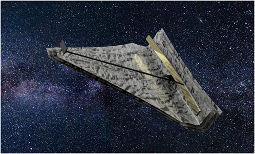
Figure 1. Concept design for a rectangular space telescope, modeled after DICER and JWST. The primary mirror is made of twenty 1 m$\times$1 m beryllium mirror segments. Scaling from JWST, the secondary mirror is 1 m$\times$2.3 m and deployed about 23 m away and offset from the primary mirror. The sunshield is meant to allow observations in all sky directions, though mirror position angles will be limited in directions that are at large angles from the antisolar point. During launch, two 10 m sections of mirrors can be folded with the reflective sides together, next to the secondary mirror support and a folded sunshade. After the two mirrors unfold, the secondary mirror beam extends out, dragging the triangular portion of the sunshade with it. The folded payload could reasonably fit in a space that is 11 m$\times$2.5 m$\times$2.5m, plausibly fitting in a Falcon Heavy launch vehicle.

The sunshield concept presented in Figure 1 extends 2 m past the ends of the primary mirror, and curls behind the secondary support and up to the secondary mirror. When pointed within 25$°$ of the antisolar point (away from the Sun), the portion of the sunshade behind the mirror will shield all of the optical elements at all rotation angles of the primary mirror. When pointed perpendicular to the plane of the ecliptic (the worst case), the triangular portion will shield the optical elements for 120$°$ of primary mirror position angle, which would easily allow the spacecraft to obtain two images separated by a 90$°$, as required for our baseline exoplanet search. For launch, we imagine that two 10 m portions of the primary mirror are folded with their reflective surfaces towards each other, the secondary mirror support is compressed to about the same length of 10 m, and the triangular portion of the sunshield is folded up. Note that both the primary mirror and the sunshield would require far less folding than JWST to fit in a launch vehicle, and require far fewer steps to unfold after launch. We estimate the size of the folded spacecraft as 11 m long (10 m of mirrors plus the thickness of the secondary mirror, the thickness of the sunshield, and possibly additional room for power, communications, and instrument packages), 2.5 m wide (slightly larger than the width of the secondary mirror), and 2.5 m deep (the thickness of two primary mirror segments folded together, plus the sunshield behind them, and imagining the power, communications and instrument packages will also need some space). This is of course a very rough estimate.

Although there are many coronagraph designs that work with conventional telescopes, we have assumed a coronagraph of type AIC. With AIC, the focal plane contains two images of the exoplanet, separated by twice the angular separation of the exoplanet and the host star. The PSF of each exoplanet image has an elongated profile determined by the diffraction limit of the rectangular mirror: 0.1″$\times$ 2″. AIC is capable of nulling over a 25% bandwidth (Gappinger et al., 2009), which covers the 1.8$\mu$m range of the MIRI F1000W filter we are assuming for our observations, but it can be tuned to other wavelength ranges. The coronagraph would need both active cooling and active correction of the path length. An optical schematic is given in Figure 2.

Figure 2

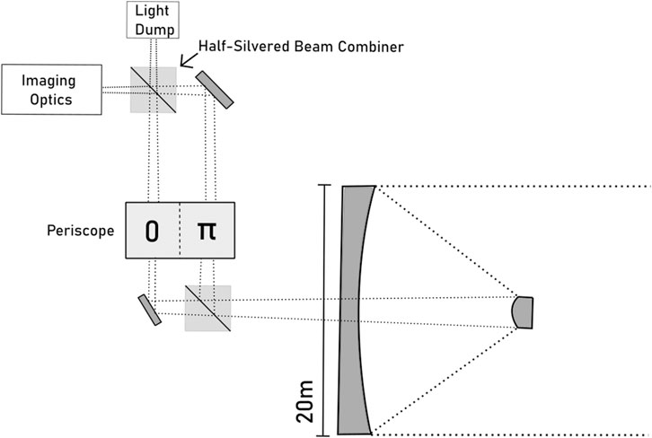
Figure 2. Schematic diagram for a rectangular space telescope with conventional mirror design (not to scale). The 20 m primary mirror is shown edge-on. The secondary mirror is 1 m$\times$2.3 m and deployed about 23 m away. Light is focused to an AIC coronagraph; half of the beam goes through a pi phase shift and the other does not. The phase shift can be accomplished with periscope optics, or by sending one of the beams through focus. The beams are then recombined with a loss of all of the coherent light. Since the path length of the light from the host star is the same in both paths, it will be removed as coherent light.

We are also assuming that the detectors are state-of-the-art single photon detectors: transition edge sensors (TES, Nagler et al., 2018; Höpker et al., 2019; Nagler et al., 2021), superconducting nanowire single-photon detectors (SNSPD, Wollman et al., 2021; Verma et al., 2021; Lita et al., 2022), or mid-infrared kinetic inductance detectors (MKID, Ras et al., 2024). With these detectors, all photons are collected without the introduction of noise; the only noise comes from zodiacal light in the Solar System and the exoplanet host system.

4 Feasibility study

The development of an optimal survey strategy and detailed throughput information for each observation is beyond the scope of this work. For example, it would require determining the best strategy to observe each known star so that the local zodiacal light is a minimum. Here, we present only a simple calculation to elucidate the capabilities of this system. Note that this study closely follows the feasibility simulation done by Swordy et al. (2025) for DICER, but we repeat the steps here for clarity.

4.1 Simulated exoplanets

We generated a simulated set of habitable exoplanets around actual Sun-like stars in the solar neighborhood. Compiling a list of Sun-like stars within 10 pc of the Earth, and meeting the needs of a particular survey, is a surprisingly complex endeavor. This is in part because information about each star is constantly being updated, and in part because the nomenclature and tabulated information for binary stars is confusing, incomplete, and often contradictory. We have attempted here to generate a reasonable set of target stars for demonstration purposes, but more work would be required to mount an actual survey.

We started with the list of 2,398 stars from the Exoplanet Direct Imaging Mission Planning Catalog (ExoCat) of stars within 30 pc compiled by M. Turnbull (Turnbull, 2015). We then restricted the dataset to the 185 stars within 10 pc, using the ExoCat distances. We then restricted the dataset to the 68 of those stars that had F, G, or K spectra as determined by ExoCat. We then modified this original list based on more modern measurements. Six of the stars had distances determined by Gaia EDR3 (Gaia Collaboration, 2020) that were much larger than 10 pc, so they were removed. Ten stars were removed because their spectral types, as compiled in the SIMBAD astronomical database (Wenger et al., 2000) were not F, G, or K. Five stars were removed because they were closer than 1″ to another star in their binary system, according to the Sixth Catalog of Orbits of Visual Binary Stars (WDS-ORB6, an updated version of the Fifth Catalog, Hartkopf et al., 2001). This leaves 47 stars from the original ExoCat list that fit all of our criteria and were used for our exoplanet detection simulations.

We then searched through SIMBAD and found 11 additional stars to include in the list. In some cases, they are stars for which the distance from the Sun decreased in Gaia EDR3 compared to the original measurements included in ExoCat. Some of the added stars are the fainter stars in binary systems. The list of stars thus increased to 58 Sun-like stars within 10 pc of the Sun, that are at least 1″ from any binary companion. The temperatures and distances to these stars are shown in Figure 3.

Figure 3

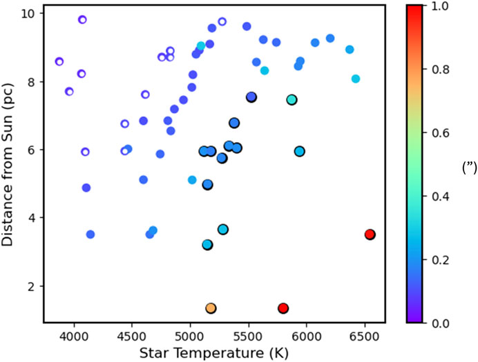
Figure 3. Target stars. We show the distances and temperatures of the 58 F/G/K stars within 10 pc of the Sun. The points are colored by the angular distance from the host star to the middle of the habitable zone, as observed from the Sun, in arcseconds. Typically, closer, hotter host stars have a larger angular distance to the habitable zone, but there is some variation due to stellar radius. Twelve stars with a calculated angular distance to the center of the habitable zone, as described in the text, that is smaller than 1″ are indicated by rings instead of filled circles and are excluded from our sample. The fifteen stars in the nearby sample are encircled by a black ring.

When simulating exoplanets around these 58 stars, we noticed that some of the habitable exoplanets were inside our coronagraph inner working angle of 0.05″. To eliminate these, we removed K stars if the average of the minimum and maximum radius of the habitable zone was less than 0.1″, as determined from (Kopparapu et al., 2013); the inner HZ was calculated using the Moist Greenhouse parameters and the outer HZ was calculated using the Maximum Greenhouse parameters from that paper, using the temperature and luminosity of each star from ExoCat. The center of the HZ was calculated as the average of these two values. If the angular distance between the star and the center of the HZ, as observed from the Sun, was less than 0.1″, then the star was removed from the sample. This removed some of the cooler K stars, particularly those that are further from the Sun. The 12 stars removed (rings in Figure 3) were: HD 4614B, HD 131156B, HIP 113283, HIP 85295, HIP 113576, HD 32450A, HIP 32984, HIP 23311, HD 38392, HIP 81300, HIP 82003 and HIP 84478, leaving us a sample of 46 target stars.

Since compiling our list, a list of HWO ExEP Precursor Science Stars (Mamajek and Stapelfeldt, 2024) was published. This list includes 51 stars closer than 10 pc. There are six stars that we selected that they do not have (HIP 5336, HIP 12114, HIP 37297, HIP 86974, HD 156384A, and HD 156384B). There are eleven stars on their list that we did not include: three stars (HIP 54035, HIP 114046, and HIP 105090) were not included because SIMBAD lists them as spectral type M, one was eliminated because it is a close binary (HIP 7981), and seven were eliminated because the calculated center of the HZ was within 0.1″ of the host star (HIP 32984, HIP 81300, HIP 84478, HIP 113283, HD 38392, HD 131156B, and HIP 23311). Although one could make different choices in the selection of the input star list, there are no additional stars in the HWO ExEP Recursor Sceince Stars list that we have not considered.

We also selected a subset of 15 of these stars that are within 8 pc of the Sun and have temperatures of $5100<T_{\mathit{\text{eff}}}<6600$ K. The 15-star list is the same one used by Swordy et al. (2025) to evaluate DICER. They represent a set of stars that are slightly closer and have temperatures that are more similar to the Sun.

Clearly, we have not heavily optimized the target list for a comprehensive exoplanet discovery mission; the temperature range of host stars could be wider, and wider separation planets could be identified around more distant stars. However, this set will give us a sense of the sensitivity of our proposed telescope to the most valuable targets.

To generate simulated exoplanets, we used the lower yield Bryson et al. (2021) model, as implemented in the P-pop exoplanet simulation tool (Kammerer et al., 2022), to simulate habitable exoplanets orbiting each of the stars. Only habitable exoplanets on circular orbits are simulated. Using the Kepler DR25 dataset, the model estimates through Approximate Bayesian Computation (Hsu et al., 2019) that, on average, each Sun-like star hosts about one planet in the habitable zone. Of our 46 target stars, 42 were included in the P-pop ExoCat_1 input catalog that is distributed with the P-pop code. Of those 42 stars, we only changed the spectral types of HIP 84720 and HD 156384A, which were originally listed as M0V and M1.5V, respectively, to the SIMBAD values of G9V (Corbally, 1984) and K3 (Bidelman, 1985). The P-pop input data for HD 10360, HIP 88601B, HD 155885, and HD 156384B came from the HWO ExEP Precursor Science Stars; these stars did not have 2MASS magnitudes because they were not resolved by 2MASS.

To achieve better statistics, the simulation was run 1,000 times, simulating 1,000 universes. Using this tool, 13,624 habitable zone planets were generated (about one planet per star per universe) around the list of 15 stars closer than 8pc, and 45,652 habitable zone planets were generated around the list of 46 stars closer than 10pc. The masses and surface temperatures of the simulated planets, as well as the temperatures of the host stars, are shown in Figure 4.

Figure 4

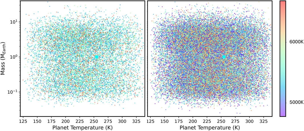
Figure 4. Simulated exoplanets. The left panel shows the mass, temperature, and host star temperatures (color bar) for 13,624 simulated habitable exoplanets orbiting 15 Sun-like stars closer than 8 pc. The simulation was done for 1,000 universes, so in our Universe we expect about 1,000 times fewer exoplanets than were simulated, or about one habitable exoplanet per host star. The right panel shows the same information for 45,652 simulated habitable exoplanets orbiting 46 F, G, K stars closer than 10 pc. Note that the larger sample of host stars includes not only more distant target stars but also a wider range of host star temperatures; in particular there are a larger number of cooler host stars. The blue cyan dot in each panel shows the mass and effective blackbody temperature of the Earth (255 K, assuming and albedo of 0.3).

4.2 Exoplanet discovery

Since we imagine using this telescope to search for previously unknown exoplanets, we will not know in advance where the exoplanet is in relation to the host star. Because a rectangular telescope has a higher resolution in the direction of the long dimension of the mirror, we need to take two images with the telescope’s primary mirror rotated by $90°$ between the two images. This way, we can discover exoplanets outside of a 0.1″ square, centered on the host star. One could instead rotate through a set of smaller (or continuous) angles to instead exclude a circular region inscribed in the square; while there might be engineering design reasons for a continuously rotating telescope, there is very little advantage in terms of exoplanet detection. If the exoplanet has already been identified, the telescope can be rotated so that its position with respect to the host star is aligned with the long axis of the mirror so that it can be most efficiently detected.

For a telescope that is 20 m by 1 m, all exoplanets further than 1″ from the host star will be distinguishable, regardless of the angle at which the telescope is rotated. All exoplanets closer than 0.05″ to the host star will not be detected, regardless of mirror rotation. For exoplanets with a separation of $0.05<\theta <1$, the detectability will depend on the orientation of the telescope and the brightness of the host star, exoplanet, and background. The larger the angular separation, the more likely the exoplanet will be detected, assuming a random telescope orientation.

The left panel of Figure 5 shows in red and orange the angular positions at which light from an exoplanet would be transmitted, and not nulled by AIC. The transmission function for this optical design is given by:

$T=\frac{1}{2}{I}_{0}LW\left(1-\frac{\sin \left(2\pi W\beta /\lambda \right)}{2\pi W\beta /\lambda }\frac{\sin \left(2\pi L\alpha /\lambda \right)}{2\pi L\alpha /\lambda }\right),$

where $\alpha$ is the angular sky position of the exoplanet in the direction aligned with the long axis of the telescope, $\beta$ is the angular sky position perpendicular to that direction, L and W are the length and width of the primary mirror (in this case 20 m and 1 m, respectively), and the observed wavelength $(\lambda )$ is 10$\mu$m. The leading factor of a half is included because AIC detects at most half of the photons that are incident to the system. Because the AIC papers derive transmission functions only for circularly symmetric apertures, we derived the transmission function following the derivation in Sections 3, 4 of Swordy et al. (2025). Because the design of DLC is parallel to the design of AIC, the transmission function math is very analogous. The only difference between the mathematics of our transmission function derivation and that of DLC is that the integration is over an $L\times W$ rectangle instead of a square with sides $D$. Since the integrals are all separable in the $X,Y$ plane, the math is identical, except that in the part of the integration associated with the $X$-direction, $D$ is replaced by $L$, and in the part of the integration associated with the $Y$-direction, $D$ is replaced by $W$. If $X$ is along the long axis of the primary mirror, then $\alpha =({\delta }_{0x}-{\delta }_{1x})/f$ and $\beta ={\delta }_{0y}/f$. Using these substitutions, our derived transmission function is similar to the rectangular transmission function corresponding to Equation 9 of Swordy et al. (2025).

Figure 5

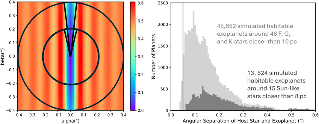
Figure 5. The effect of exoplanet position on planet detection. The left panel shows the AIC transmission fraction (The maximum AIC transmission is $\sim$0.5 because half of the light is lost in combining the two beams) as a function of the relative sky position of the planet with respect to the star. Here, $\alpha$ is the angle in the sky that is aligned with the long axis of the mirror, and $\beta$ is the angle in the sky that is perpendicular to that. If the telescope rotates while staring at the host star, the planet traverses the transmission plane in a circle with a radius given by the angular separation between the star and the planet. The two circles shown in the panel correspond to star-exoplanet separations of 0.2″ and 0.4″. For smaller angular separations, the planet spends a larger fraction of the time in the low transmission (blue) region of the focal plane where it cannot be detected. The histograms in the right panel show the distribution of angular distance from the host star for 45,652 simulated habitable exoplanets orbiting 46 F, G, K stars closer than 10 pc (light gray), and also for the 13,624 simulated exoplanets orbiting 15 Sun-like stars closer than 8 pc (dark gray). The simulation was done for 1,000 universes, so in our Universe we expect about 1,000 times fewer exoplanets than were simulated, or about one habitable exoplanet per host star. The simulation creates only circular planet orbits, which we view at any orientation, so the angular separation represents the largest angular separation that the planet will have on its orbit. Simulated exoplanets that have a maximum separation of less than 0.05″ are not detectable; note that the target host stars were selected in temperature and distance so that their habitable zones are nearly completely detectable.

The right panel of Figure 5 shows the maximum angular separation between the simulated exoplanets and their host stars. Because the exoplanet simulator only models circular orbits, the projected path of the exoplanet on the sky is an ellipse with a semimajor axis that is set by the radius of the exoplanet’s orbit and the distance from us to the host star, and an eccentricity that is set by the inclination of the orbit. The figure shows that the inner working angle (0.05″) for the AIC coronagraph and a 20 m mirror is small enough that almost all of the simulated habitable exoplanets are observable. However, exoplanets with orbital planes that are inclined to our line-of-sight might not be visible at all points in their orbits. Repeat observations, at times when the exoplanets are at different positions in their orbital paths, would allow us to trace planetary orbits and identify planets in edge-on or eccentric systems that are sometimes too close to the host star to detect.

Planets that are too close to the host star (hot) will not be resolved, and planets that are too far away (cold) will not emit significant light at 10 $\mu$m; because of this, this rectangular infrared space telescope preferentially finds only habitable zone planets.

4.3 Simulated exoplanet yield

We calculated the number of simulated exoplanets that we would detect with a rectangular infrared telescope. Given the simulated exoplanet temperatures and radii, we calculated the angular distance from the host star, the blackbody flux at 10$\mu$m, the subtended solid angle of the host star, and the planet flux as observed from the Earth. We then compared this planet signal with the background noise from stellar leakage and zodiacal light. For example, we calculate that a 256 K blackbody planet with the radius of the Earth, at a distance of 7.5 pc, would produce $\sim$17,000 photons per hour. (Though note that the actual Earth emission is somewhat higher at 10$\mu$m than the blackbody emission for an equivalent total emission object with a temperature of 256 K.) In this section, all calculations were done assuming that the bandwidth of the observations is 1.8$\mu$m, similar to the MIRI F1000W filter. The central wavelength of the observations was assumed to be 10$\mu$m. We multiplied the planet flux by the transmission function (Figure 5) and by the fraction of the planet’s light that would be within the diffraction-limited resolution of the telescope, which in this case is 0.737.

The optimal transmission function for the system was assumed to be 25%, including 50% from loss in the AIC beamsplitter and another 50% due to other optical elements (equal to the overall throughput of JWST; Giardino et al., 2022). Note that transmission might be improved by using detector efficiency from TESs, SNSPDs, or MKIDs.

The main source of background is zodiacal light from the Solar System or from the exoplanet’s host solar system. The local zodiacal cloud varies in brightness as a function of position in the sky, and depends on the relative position of the Sun and Earth (and therefore the time of year). It is typically brighter towards the Sun (where the dust is hotter) and near the plane of the ecliptic. Using IRAS data (Schlegel et al., 1998) and the NASA Euclid background model tool (Euclid Background Model, 2017), we estimated that when observing from L2, the local zodiacal light background varies between 10 and 20 MJy/sr. Unless the exoplanet system is located very near the Celestial Equator, there is an optimal time of year when it can be observed with $\sim$10 MJy/sr of local zodiacal light background, which is what we assumed in the signal-to-noise calculation.

It is difficult to estimate the zodiacal dust background that comes from the exoplanet system itself, because habitable zone zodiacal dust has been observed in very few systems. While there are dozens of systems that have zodiacal light that is known to be orders of magnitude brighter than in the Solar System (di Folco et al., 2007), it is possible that these are unusual systems for which the zodiacal dust has been detected because it is so bright. Adding to the uncertainty, it matters how the exozodiacal dust is distributed in the host system. If it is concentrated close to the host star, it will be nulled. If it is preferentially in the same plane as the exoplanet, it would be preferentially located near the exoplanet, especially in edge-on systems. The Large Binocular Telescope Interferometer (LBTI) Hunt for Observable Signatures of Terrestrial Systems (HOSTS, Ertel et al., 2020) survey found zodiacal dust in four out of 25 Sun-like stars observed. By fitting the luminosity function of the observed light, they estimate that the typical Sun-like star has a zodiacal dust emission similar to our own Solar System, with a median habitable zone zodiacal dust level of three times that of the Solar System. With one sigma error bars, the median habitable zone zodiacal dust level is less than 9 times that of the Solar System.

In our signal-to-noise estimates, we assumed that the exozodiacal light in the region around the exoplanet has twice the surface brightness as the minimum local zodiacal light. This estimate is very uncertain, but is justified by the following argument. The whole range of surface brightness from the local zodiacal dust is $10-20$ MJy/sr, including towards the Sun, towards the plane of the ecliptic, and looking out of the plane. If the surface brightness of dust looking through a disk is twice as high as looking out of a disk from the midplane (where the zodiacal light background is low), then the surface brightness looking through a disk is about the same as the highest zodiacal backgrounds in the Solar System. Since surface brightness is independent of distance, the exozodiacal light background is also independent of distance to the host system, as long as the planet is located within a disk of zodiacal dust. The estimate of 20 MJy/sr for exozodiacal dust could be optimistic or pessimistic, since the amount and distribution of exozodiacal dust in each system is not known; it is possible that much of the exozodiacal dust (including much of the brighter, hotter dust near the star) could be nulled along with the host star light.

We used 30 MJy/sr for the total zodiacal light background for all of the simulated exoplanets. This amounts to $\sim$15,000,000 photons per hour in a $2\times 0.1$″$\times$2″ region. The first factor of 2 comes from the two exoplanet images in the focal plane, that in AIC often do not overlap). The angular resolution in the long direction of the mirror is $0.1$, and the resolution in the short direction of the mirror is $2$. At a particular sky position, the total zodiacal light background is multiplied by the transmission function (Figure 5); zodiacal light close to the host star is nulled along with the host star light.

Background can also be contributed by the host star itself from stellar leakage, pointing jitter, or residual optical path difference. The stellar leakage was calculated using:

$I_{0}LW{\pi }^2{r}_{\ast }^2\left[L^2+W^2\right]/12{\lambda }^2.$

This was computed using the small angle approximation of our transmission function:

$T\left(\alpha ,\beta \right)=I_{0}LW{\pi }^2\left(L^2{\alpha }^2+W^2{\beta }^2\right)/12{\lambda }^2,$

which includes a factor of 1/2 for the transmission loss in beam combining. The star was assumed to emit $I_0$ uniformly over a disk of angular radius $r_{\ast }$, so the leakage is the integral of the transmission function over the stellar disk divided by $I_0\pi r_0^2$. A G star at a distance of 7.5pc would produce $1.0\times 10^{11}$ photons per hour. The stellar leakage is only 3,200,000 photons per hour (a factor of $3.2\times 10^{-5}$ suppression of the starlight).

If the planet is located inside of half of the diffraction limit of the telescope, then it will be impossible for us to determine the background level from stellar leakage, and the planet is assumed to be impossible to observe. If the planet is outside of half of the diffraction limit, then it is assumed that the background can be determined with very little error. The amount of light in the pixel(s) in which the planet light is captured is found by integrating a normalized Gaussian with sigma of 0.34 times the diffraction-limited resolution:

$L_{\mathit{frac}}=2{\int }_{X-{\theta }_L/2}^{X+{\theta }_L/2}G\left(X^{\prime },0.34\lambda /L\right)d{X}^{\prime }{\int }_{Y-{\theta }_W/2}^{Y+{\theta }_W/2}G\left(Y^{\prime },0.34\lambda /W\right)d{Y}^{\prime }.$

Here, $L_{\mathit{frac}}$ is the fraction of leaked light that overlaps with the planet. The factor of 2 is there because there will be two images of the planet in the focal plane. The primary mirror has length $L$ and width $W$. The angular position of the exoplanet with respect to the host star is $(X,Y)$, where $X$ is in the direction of the long axis of the primary mirror and $Y$ is in the direction of the short axis of the primary mirror. $G(X,\sigma )$ is a normalized Gaussian centered on zero with a width given by $\sigma$. The $\sigma$ of the Gaussian in each direction is calculated as 0.34 times the diffraction limit in the direction being integrated over; the factor of 0.34 is a standard assumption for the fit of a Gaussian to the Airy function.

We did not include star background from pointing jitter or residual optical path difference, because we expect these to be much smaller than either the zodiacal light background or the stellar leakage; it is not expected that this approximation will significantly affect our results.

For the case of an Earth-like planet orbiting a Sun-like star at a distance of 7.5 pc, and with the position angle of the planet aligned with the long axis of the telescope, the estimated flux for the exoplanet, zodiacal light and star are 15,000, 18,000,000 and 1,900,000 photons per hour. The primary source of noise is zodiacal light. For different stars, exoplanets, and telescope position angle, the stellar leakage can vary widely. The signal-to-noise ratio (SNR) is calculated as:

$SNR=R_{p}t/\sqrt{\left(R_p+R_z+R_s\right)t},$

where $R_p$, $R_z$, and $R_s$ are the rates at which photons are collected from the planet, zodiacal light, and stellar leakage, respectively. $t$ is the exposure time of the observation. In this case, for an exposure of 1 day, the SNR is seventeen.

We estimated the output of a very simple survey strategy, in which each star is observed for the same amount of time. In practice, we expect the time to completion (or alternatively the number of identified exoplanets) could be significantly improved with an adaptive approach that uses different exposure times based on the host star’s distance and temperature, and that uses the results of previous observations of each star to inform future observations.

We first imagine searching for the 13,624 simulated exoplanets simulated around 15 nearby Sun-like stars, trying a range of different exposure times up to 40 days. With longer exposure times, fainter (lower mass and lower temperature) exoplanets can be discovered. Each planet was assumed to have a circular orbit. A random angle between 0 and 2$\pi$ was selected to represent the position of the planet on the orbit. A random angle between 0 and $\pi /2$, weighted by $\sin (i)$, was generated to indicate the inclination of the orbit to our line of sight. A random angle between 0 and $\pi$ was generated to indicate the angle between the long angle of the ellipse that the planet traces on the sky and the long axis of the telescope mirror. For each planet, a particular $(\alpha ,\beta )$ was calculated from these three random angles, where the angles are measured from the host star. $\alpha$ is the angle in the direction of the long axis of the telescope mirror, and $\beta$ is in the direction of the short axis of the telescope mirror, as pictured in the left panel of Figure 5.

From these $(\alpha ,\beta )$ values, the properties of the host star, and the properties of the simulated exoplanets, we calculated a SNR for each exoplanet, as outlined above. For each exposure time listed, the sky is exposed for half of that time in one random position angle of the primary mirror, and then the other half of the time it is exposed with the primary mirror rotated by $90°$. The SNR is calculated by adding together the photons from the planet as calculated from each of the two exposures, and then dividing by the square root of the sum of the photons from the planet, zodiacal light, and stellar leakage from the two exposures.

Figure 6 shows the calculated SNR as a function of the maximum angle between the exoplanet and the host star for both of the star samples. The left panel shows 10 days of observation for each of the fifteen closer stars, and the right panel shows 10 days of observation for each of the stars in the larger sample of 46 stars that extends out to distances of 10 pc. There is a maximum and minimum angular distance from the host star that depends on the temperature of the host star (and therefore the range of orbital radius in the habitable zone) and the distance (which determines the angular separation). The exoplanets that are closer to the host star are hotter and therefore brighter; if the closer exoplanets are far enough from the host star that they can be resolved, then they have a higher SNR. Many of the exoplanets are detected with extremely high SNR.

Figure 6

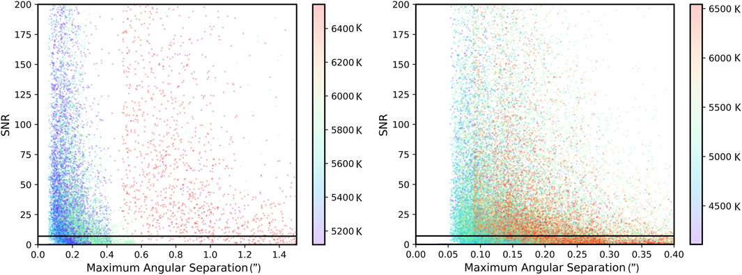
Figure 6. SNR as a function of the maximum angular separation (in arcseconds) for a 10 day exposure time. We use a SNR of 7 (horizontal line) as a detection limit. For each of the 13,624 exoplanets simulated around 15 nearby Sun-like stars, we calculated the SNR ratio when the planet was in a random orbital phase, at a random inclination, and viewed at a random position angle. Note that if the planet happens to be closer than 0.05″ to the host star at this particular place on its orbit, it will be unresolved and the SNR will be zero. The left panel shows the calculated SNR for a 10 day exposure time, with the points color-coded by the surface temperature of the host star. For example, the red points in the left panel represent all of the exoplanets simulated in $\sim$1,000 universes that are orbiting one star. Because the simulation only generates planets in the habitable zone, there are no simulated exoplanets within $\sim 0.5$″ of the host star. The exoplanets that are closer to the host star are generally hotter and therefore brighter than the more distant exoplanets, so they have a higher SNR. Smaller exoplanets that are in the outer part of the habitable zone are more difficult to find. The right panel shows the SNR versus maximum angular separation for the 45,652 simulated exoplanets orbiting 46 stars closer than 10 pc from the Sun. This simulation includes all of the stars in the smaller sample, but also includes more distant stars with habitable zones that have a smaller angular separation. We chose to show only the simulated planets in the inner 0.4″ for this panel so that more of the closer exoplanets could be distinguished. Note that the color bars of the two plots are different because the temperature range of the stars in the two samples are different.

Figure 7 (left panel) shows the exoplanets detected at a 7 sigma level given the exposure time, the randomized position of the exoplanet with respect to the host star, the properties of the host star and simulated exoplanet, and their distance. Of the 13,624 simulated planets, 8,883 were found with a 2 day integration time on each host star (red), 9,658 were found in 4 days of integration (orange), 10,093 were found with 6 days (green), 10,394 were found with 8 days (blue), and 10,511 were found with 10 days (light gray). Each of these exoplanet yields must be divided by 1,000 (number of simulated universes) in order to estimate the actual yield. This panel can be compared with the 80 day exposure DICER detections in the right panel of Figure 16 of Swordy et al. (2025); note that the mirrored telescope finds more than twice as many exoplanets, including lower mass, cooler exoplanets, and exoplanets with a smaller exoplanet-host star separation, in a fraction of the time. Because the exoplanet phase, inclination, and position angle are chosen randomly, the exact number of exoplanets discovered is slightly different each time the selection program is run.

Figure 7

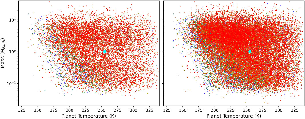
Figure 7. Exoplanets detected at the 7 sigma level with the rectangular mirror space telescope. On the left, we show exoplanet detections in 10 days of exposure time for 15 nearby Sun-like stars (closer than 8 pc), simulated 1,000 times each. Of the 13,624 simulated planets, 8,883 were found with a 2 day integration time on each host star (red), 9,658 were found in 4 days of integration (orange), 10,093 were found with 6 days (green), 10,394 were found with 8 days (blue), and 10,511 were found with 10 days (light gray). On the right, we show exoplanet detections in 10 days of exposure time for 46 F, G, or K stars within 10 pc, simulated 1,000 times. Of the 45,652 simulated exoplanets, 20,492 were found with a 2 day integration time on each host star (red), 23,306 were found in 4 days of integration (orange), 24,908 were found with 6 days (green), 26,019 were found with 8 days (blue), and 26,682 (light gray) were found with 10 days. With the larger sample of nearby stars (where 27 exoplants are found in one universe), we show that the rectangular infrared telescope can feasibly meet the HWO goal of finding $\sim$25 nearby, habitable exoplanets.

This calculation shows that in 10 days of exposure time on each of 15 Sun-like stars (0.4 years of exposure time), we expect to find 11 habitable exoplanets. About 83% (66 out of 80) of the simulated exoplanets with radii, masses and temperatures similar to the Earth ($0.9<R_p/R_{\oplus }<1.1$, $0.9<M_p/M_{\oplus }<1.1$, and $250K<T_p<300K$) were detected. The number of detected planets as a function of the planet’s angular separation from the host star is shown in the left panel of Figure 8.

Figure 8

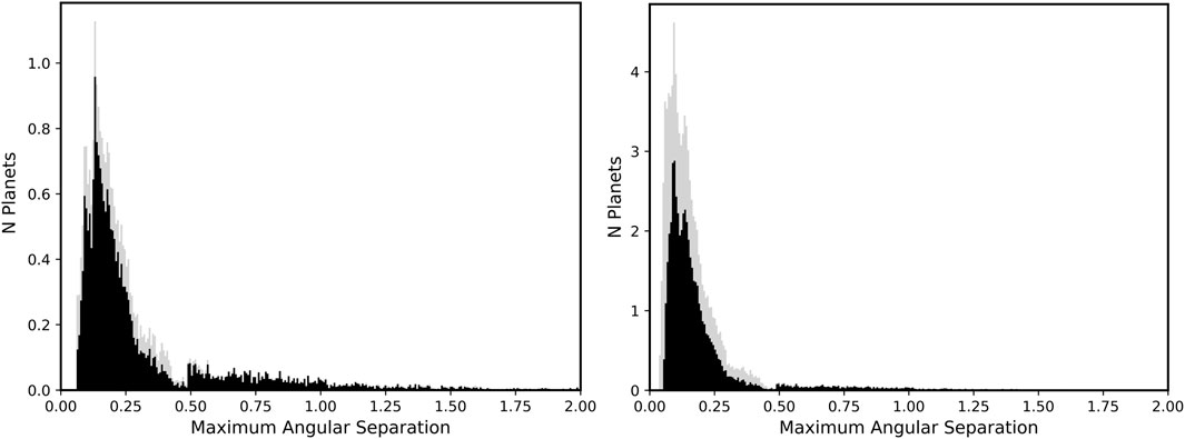
Figure 8. Efficiency for finding exoplanets as a function of separation from the host star in arcseconds. In the left panel we show in gray the distribution of maximum angular separation for the 13,624 simulated planets orbiting 15 nearby, Sun-like stars. In black, the distribution of exoplanets that are above a 7-sigma detection limit with 10 days of exposure on each star is shown for comparison. The right panel shows the distribution of maximum angular separation for the 45,652 simulated planets orbiting 46 nearby stars (gray), along with the distribution of exoplanets that are above a 7-sigma detection limit with 10 days of exposure. Note that in both cases we can find exoplanets all the way in to the diffraction-limited resolution of 0.05″.

We then imagined searching for the 45,652 exoplanets simulated around 46 F, G, or K stars within 10 pc. Figure 7 (right panel) shows the exoplanets detected at a 7 sigma level given a range of exposure times between 2 days and 10 days. Of the simulated exoplanets, 20,492 were found with a 2 day integration time on each host star (red), 23,306 were found in 4 days of integration (orange), 24,908 were found with 6 days (green), 26,019 were found with 8 days (blue), and 26,682 (light gray) were found with 10 days.

This calculation shows that in 10 days of exposure time on each of 46 selected stars closer than 10 pc (1.3 years of exposure time), we expect to find 27 habitable exoplanets. About 71% (198 of 278) of the simulated exoplanets with radii, masses and temperatures similar to the Earth ($0.9<R_p/R_{\oplus }<1.1$, $0.9<M_p/M_{\oplus }<1.1$, and $250K<T_p<300K$) were detected. Note that many of the detections (right panel of Figure 8) are closer than 0.1″ from the host star.

Because the exozodiacal light is so poorly understood, we explored how a much brighter exozodiacal light background would affect the results. Previously, we assumed that the amount of zodiacal dust in the host exoplanet system was the same as in the Solar System. For comparison, we will now assume that the exozodiacal light is ten times as large as in the Solar System, so that the total zodiacal light background is 210 MJy/sr. In this high exozodiacal light regime, instead of finding 27 exoplanets around 46 nearby stars with 10 days of exposure each, we would find 20 planets. If we increased the exposure time by a factor of 6 (60 days each), we would recover the original 27 exoplanets. From this, we conclude that the exozodiacal dust significantly affects the detection of habitable, Earth-like worlds; but within current expectations for the amount of exozodiacal dust, a rectangular telescope of this design would still be successful.

4.4 Measuring biomarkers

Once habitable exoplanets are identified, it is important to then be able to obtain information about their planetary atmospheres in order to identify biomarkers. While it is possible for exoplanets to contain oxygen in their atmospheres without the presence life, abiotic mechanisms are not expected to sustain oxygen in atmospheres of Earth-like habitable planets orbiting Sun-like stars for a sustained period of time (Meadows, 2017). In the case of the Earth, the ozone in the Earth’s atmosphere was created from oxygen that was released through photosynthesis. Therefore, finding ozone in the atmosphere of a habitable planet would be a strong indicator of life and in particular of life that uses and stores energy from the host star through photosynthesis (on Earth photosynthesis occurs in vegetation and micro-organisms).

Because the AIC can only null over a 25% bandwidth, we assume that in each exposure we will only be able to obtain spectra over a wavelength range of 2.5$\mu$m in the infrared. For our simple calculations, we are assuming we wish to only identify the $O_3$ absorption band at 9.6$\mu$m; the entire width of this band, including some continuum on each side, can easily be obtained within the spectral bandwidth of one observation with a simple mid-infrared spectrograph. Since spectroscopy would only be done once exoplanets are detected, we could rotate the telescope mirror so that the long axis of the mirror points along the direction from the star to the exoplanet, for maximal separation of the two objects, and we could transmit to the spectrograph only the photons within the resolution of the habitable exoplanet. We note that like JWST, it would be possible to include multiple instruments that cover a wider range of infrared wavelengths. However, that is not necessary to achieve our stated science goal.

We imagined obtaining spectra of the $O_3$ absorption line for the 10,511 habitable exoplanets detected from the 15 stars closer than 8pc in 1,000 realizations of the Universe with an effective observation time of 10 days per host star. While it is easy to design a spectrograph with higher resolution, the photon flux from exoplanets is so low that we expect to look just for a detection of a lower number of counts in the 0.6$\mu$m-wide absorption line. We aimed to detect a flux that is half of the blackbody signal at 10$\mu$m, in a bandwidth of 0.6$\mu$m (the width of the line), with a signal-to-noise ratio (SNR) of 5. In most other respects, the calculation is the same as the calculations of SNR for the photometry. The average exposure time to get a 5$\sigma$ detection of the $O_3$ absorption line is 4 days; the SNR for the continuum on either side of the line will have much higher signal-to-noise. For the expected 11 exoplanets that would be identified in one universe, it would take 0.12 years of exposure time to search for $O_3$. Including the 0.4 years of exposure time required to detect these exoplanets, 0.5 years of exposure are required; this might be accomplished within a $\sim 1$ year mission.

For the larger sample of 46 stars, observing each star for a total of 10 days, we expect to find 27 habitable zone exoplanets within 10 pc in 1.3 years of exposure time. These discoveries could then be searched for ozone with an average of 6 days of exposure time each, requiring an additional 0.4 years of exposure time. If we could operate the telescope long enough to obtain 1.7 years of exposure time, we would achieve the HWO goal of finding at least 25 habitable exoplanets and searching them for an $O_3$ biosignature. Depending on the duty cycle, this could require about a three and a half year mission.

5 The equivalent area square telescope

For comparison, we evaluated the exoplanet-finding capability of a square telescope with an equivalent collecting area. This telescope has a “diameter” of 4.47 m. The results for the square telescope will be similar to the typical circular footprint for a telescope collecting area, and have the advantage that we can run exactly the same code with only two numbers (the length and width of the telescope) changed.

The PSF is spread over the same number of pixels either way; one resolution element in the rectangular case is ${\lambda }^2/(LW)$ and in the square case is ${\lambda }^2/{(\sqrt{LW})}^2$. Therefore, the detection of isolated point sources is about the same in either case. If the goal is to measure the detailed shape of an extended object, the rectangular telescope would require multiple pointings at different rotation angles, and a much more complex data analysis pipeline. Where the rectangular telescope design really shines is in the detection of point sources that are closer to each other than can be detected with the equivalent circular telescope. Note, however, that engineering capabilities such as mirror alignment, pointing and jitter, residual optical path length, etc., will need to be at the level (at least in one dimension) that is required for a circular telescope of diameter $L$.

With a diameter of 4.47 m, the diffraction limit is 0.46″, which means we will not be able to resolve planets that are closer than 0.23″ to the host star. This restriction makes it impossible to find most of the habitable planets we are trying to identify. For the 46 stars with 45,652 simulated exoplanets, we found 2,563 exoplanets with an exposure time of 2 days, 2,795 exoplanets with an exposure time of 4 days, 2,903 exoplanets with an exposure time of 6 days, 3,044 exoplanets with an exposure time of 8 days, and 3,144 with an exposure time of 10 days. Increasing the exposure time will not allow us to reach our goal for finding Earth-like habitable exoplanets, because most of the exoplanets we wish to find cannot be resolved from the host star with the square design and are therefore not possible to detect.

The left panel of Figure 9 shows the exoplanet temperatures and radii that we can find with the equivalent area square telescope. Note that we are preferentially losing the lower mass and warmer exoplanets, including those that are most similar to the Earth. Only 5% (14 of 278) of the simulated exoplanets with radii, masses and temperatures similar to the Earth ($0.9<R_p/R_{\oplus }<1.1$, $0.9<M_p/M_{\oplus }<1.1$, and $250K<T_p<300K$) were detected. The right panel of Figure 9 shows the distribution of angular separation between the host star and the detected exoplanets, highlighting the much larger inner working angle of this telescope footprint.

Figure 9

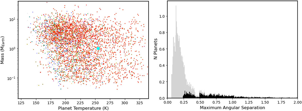
Figure 9. Exoplanet detections with an equivalent area square telescope. We consider the number of exoplanets we can discover around the 45,652 simulated planets orbiting 46 nearby stars, changing only the length of the telescope from 20m to 4.47 m and the width of the telescope from 1m to 4.47 m. We show here the equivalent area square telescope detections by reproducing the information in the right panel of Figure 7 and the right panel of Figure 8 for this primary shape. Notice that all of the exoplanets with angular separations smaller than 0.23″ can no longer be detected. That eliminates most of the habitable exoplanets that we aim to find.

6 Discussion

There is nothing about the idea of making a rectangular mirror, or the AIC coronagraph, that precludes its use at any wavelength. Any current design for HWO or any other flagship mission could be adapted to work with a rectangular primary optical element. For example, if the 20 m$\times$1 m mirror proposed here was used in the visible at 500 nm, the images could in principle be 0.005″ × 0.05″. This would allow for the detection of Earth-like exoplanets to distances of about 200 pc (twenty times farther, because the wavelength of the light is 20 times shorter). We note, however, that there would be considerably more stellar leakage, and the constraints on pointing and stability would make construction much more difficult.

We also point out that the proposed infrared survey for exoplanets favors the detection of habitable exoplanets, with only modest coronagraph performance. Planets that are much cooler than the Earth will be very faint at 10$\mu$m, and therefore much more difficult to detect. Planets that are much warmer than the Earth will be closer to the host stars, and therefore less likely to be resolved. The extremely faint, habitable exoplanets are detected at their most luminous wavelength.

In general the design of a rectangular telescope can be adapted to favor discovery of any particular exoplanet type, at any distance. It can also be designed to enable detailed followup for discovered exoplanets, in which case one would be able to orient the long axis of the mirror in the direction of the current position angle of the exoplanet for maximum resolution. Resolving an exoplanet from its host star is the first step to any exoplanet observation, and for fixed mirror area the highest resolution can be obtained with a rectangular shape. It is instructive to compare the rectangular mirror infrared telescope with other concepts that are being considered for habitable exoplanet discovery.

The Large Interferometer For Exoplanets (LIFE, Quanz et al., 2022; Dannert et al., 2022) collaboration is exploring the use of an array of smaller space telescopes that fly in formation to very high precision. LIFE benefits from two past interferometric, planet-finding mission concepts, ESA’s Darwin (Cockell et al., 2009) and the NASA’s Terrestrial Planet Finder Interferometer (TPF-I, Beichman et al., 1999), that were canceled due to limitations of our technology and knowledge of exoplanets. Conceptually, LIFE includes four collector spacecraft that formation-fly in a rectangular array, sending light to a beam combiner spacecraft in the center. The whole array rotates to modulate the signal from an exoplanet. LIFE uses a Bracewell interferometer that is enormously expensive in terms of conops; changing the boresight direction is prohibitively expensive for use as a survey instrument. Because of this, it is better utilized for assaying promising planets that have already been detected. Our concept is more feasible because the fixed 20 m long mirror alleviates the need for formation flying, but it does not allow for baselines in the 25–250 m range imagined by LIFE.

The LUVOIR Decadal Survey Mission Concept Study (The LUVOIR Team, 2019) imagined finding and characterizing exoplanets with an 8–15 m space telescope with a coronagraph that is capable of extremely high contrast nulling. The HabEx Decadal Survey Mission Concept Study (Gaudi et al., 2020) also aimed to study exoplanets, but with a 4 m diameter telescope and a 52 m starshade that flew 76,600 km away from the telescope to enable a 0.07″ inner working angle coronagraph. These ideas are the basis of the technology development for HWO.

The Chinese Academy of Sciences (CAS) has funded a concept study for the Tianlin mission (Wang et al., 2023), a $\sim$6 m UV/Opt/NIR space telescope that is primarily designed to discover and measure biosignatures for nearby G/K stars with the direct imaging method. They aim to start operation of this 5+ year survey within the next 10–15 years. They imagine looking for water, ${\text{O}}_3$, ${\text{O}}_2$, ${\text{CH}}_4$ and chlorophyll in the planetary atmospheres. For example, a 6 m telescope fitted with a coronagraph that can suppress starlight by a factor of $10^9$ can detect water vapor in a nearby Earth-like planet orbiting a Sun-like star with about 40 days of exposure time.

The LUVOIR, HabEx, Tianlin and LIFE concepts grew out of the strong need for an exoplanet observatory with a large baseline and an efficient coronagraph with small inner working angles. The rectangular mirror design proposed in this paper would be easier to launch into space and requires a dramatically lower contrast coronagraph than LUVOIR or Tianlin. It does not require a starshade to fly thousands of miles to point from one host star to another like HabEx, and does not require formation flying like LIFE. It has somewhat more modest goals in that it targets a smaller list of nearby exoplanets and as proposed here does not really deliver spectra. However, discovering habitable planets around the closest stars to Earth arguably promises the highest reward. Our proposed design might be a simpler way to identify interesting habitable planets for later follow-up with HWO or LIFE.

The rectangular mirror telescope is not without its own engineering challenges. One such challenge that requires further study is the structural stability of the rectangular primary mirror. Thermal stability will also need to be considered. While we did not specifically address structural and thermal stability of the optics, they are design concerns because vibration in the mirrors and their support structure will cause the mirror to bend and contribute to jitter (Hyde et al., 2004) and optical thermal stability is required to control distortion. Infrared observing in particular requires a high degree of temperature control to reduce thermal backgrounds. However, it seems plausible that careful design, informed by structural models and confirmed by environmental testing (Kimble et al., 2018), will ameliorate any concern about launch loads or geometric changes in the primary mirror due to thermal gradients (Arenberg et al., 2006). We note the extensive modeling and design effort conducted by NASA to assure that JWST’s 18 hexagonal beryllium mirrors, mounted on individual hexapods, were capable of maintaining their shape in the presence of launch loads and, during operations, external thermal variability. The design we propose for the primary grating is well within NASA’s high-fidelity modeling and environmental test (cryovac and vibration) capabilities (Feinberg et al., 2024).

Although we arrived at the idea of a high aspect ratio mirror independently, we point out that we were not the first to suggest this. The Terrestrial Planet Finder (TPF) project considered two space mission design concepts: an infrared astronomical interferometer (TPF-I; Lawson et al., 2006), which imagined several small telescopes flying in formation, and a visible light coronagraph (TPF-C; Traub et al., 2006), which studied a design with a large oval telescope with a major axis of 8 m and a minor axis of 3.5 m. The oblong mirror design was proposed to reach small inner working angles while keeping the mirror small enough to be easily deployed in space. A variation of TPF-C that used a 50 m diameter disk called an occulter (Cash, 2006), flying in formation with TPF-C at a distance of 50,000 to 70,000 km, was called TPF-O, and predated the HabEx starshade. Our simple design uses a mirror that is more elongated than that of TPF-C, but operates in the infrared like TPF-I. By operating in the infrared, the requirements on the coronagraph are more relaxed, eliminating the need for an occulter.

TPF-C concentrated much more on exoplanet spectroscopy and the identification of biosignatures than we have. However, our proposed mission operations could be enhanced to include identification of other biosignature molecules (for example, Levine et al., 2006, Appendix 1.A), most notably carbon dioxide (15.0$\mu$m, 10.4$\mu$m, and 9.3$\mu$m), methane (7.7$\mu$m and 8.0$\mu$m), and water (7.0$\mu$m and 20.5$\mu$m). Because AIC only nulls over a 25% bandwidth, we are limited to a spectral bandwith of $\sim 1-5\mu$m in the mid-infrared. While a few of these absorption bands could be probed in one pointing, others would require a pointing just for that line. Details of the science case might also require measurements of the continuum, for instance to determine the temperature of the exoplanet. Alternatively, this mission could be viewed as a less expensive way to identify the most promising targets for future spectroscopic missions such as HWO and LIFE. Slewing HWO or LIFE from one pointing to the next will be enormously expensive; certainly, the LIFE conops is such that moving the rotating constellation will be very complex and require a significant expenditure of propellant.

Refinements of the science plan should also include varying the exposure time for each star, based on the star’s distance and temperature; closer, hotter stars will need less exposure time to observe exoplanets in the habitable zone. The required exposure time will also evolve as more information on exozodiacal dust, including exozodiacal dust around these stars in particular, becomes available.

In our proof-of-concept calculations, we have not considered repeat observations of exoplanets to determine their orbits. It takes observations of at least three orbital positions to determine an elliptical path of the planet in the sky, but more could be required depending on the positional accuracy of the measurements.

Figure 10 of Stark et al. (2019) shows the number of exoplanets that could be discovered in 2 years of telescope time (1 year of exposure time) as a function of telescope diameter for several popular exoplanet telescope/coronagraph/starshade designs. While our calculation uses different assumptions and is in many aspects less rigorous, it is interesting to note that our estimate of three discovered exoplanets with 1.3 years of telescope exposure with a $\sim$4.5 m telescope is similar to the number of exoplanets that Stark et al. (2019) estimated for a segmented on-axis telescope of the same diameter with an apodized pupil Lyot coronagraph. Looking at the curves for yield as a function of diameter, our yield for a 20 m$\times$1 m telescope is roughly equivalent to the yield for a 10 m diameter telescope. This suggests that if building, deploying, and operating a 20 m$\times$1 m telescope is easier and less costly than a 10 m diameter telescope, the rectangular design is preferred.

Our proof-of-concept calculations consider only optics and not the very real engineering considerations for operating a space telescope. For example, we calculated the throughput for two images taken with the mirror rotated $90°$ between the two observations. In practice, rotating a telescope–and in particular a telescope with mass distributed to large radii–could consume a considerable amount of fuel. It might be more advantageous to continuously rotate the telescope through $90°$. This will cause smearing over the distance that a point source moves in the image plane during the length of an observation. The rate at which an exoplanet will move is $v=2\pi r/T$, where $r$ is the angular distance from the host star to the exoplanet and $T$ is the rotation period, which is four times the exposure time. For a 10 day exposure time, and a large separation angle of 2″, the exoplanet moves 0.013″ per hour. If the image is read out every hour, or even every few hours, the smearing from rotation will be considerably smaller than the point spread function. This does complicate the data analysis, but if anything increases exoplanet detectability; exoplanets will be excluded inside a circular region with radius equal to half of the diffraction limit for the long axis of the telescope rather than a square with a side length of the diffraction limit for the long axis of the telescope. Exoplanets that would have landed in a place with unfavorable transmission function in one of two images will instead have a much longer effective exposure time because they will be excluded less than half of the time; in exchange, many more exoplanets will fall in the unfavorable region for a small fraction of their exposure.

7 Conclusion

In this paper, we suggest that the search for exoplanets would benefit from changing the shape of the primary collecting element to a rectangle. We show that using technology that has already been developed for JWST, we could plausibly build an infrared telescope that could achieve the HWO goal of detecting 25 habitable, Earth-like exoplanets and determine whether there is ozone in their atmospheres. Since HWO does not aim to image exoplanets in the mid-infrared, the proposed mission would not only be a precursor mission, but would also provide complementary data for future HWO observations.

The rectangular mirror telescope outlined here is an infrared space observatory with a 20 m$\times$1 m primary mirror and an AIC coronagraph. This observatory can find an estimated 11 habitable exoplanets orbiting the closest 15 stars with $5100\mathrm{K}<T_{\mathit{\text{eff}}}<6600$ K, and determine whether they have ozone in their atmospheres, in a mission of 1 year. If the mission is extended to $\sim 3.5$ years, an estimated 27 habitable exoplanets are expected from a sample of 46 F, G, and K stars within 10 pc.

These nearby exoplanets are the most precious planets to find because we will be able to study them in the most detail. The closer the exoplanet is, the more likely we could send a probe to investigate, establish communication with its residents, or possibly one day visit.

A fixed rectangular mirror allows for high resolution measurements only along the long axis of the rectangle. By taking half of the exposure time at one mirror position and half of the exposure time with the mirror rotated by $90°$ (or alternatively by smoothly rotating the telescope through $90°$ during the exposure), we can achieve most of the resolution for finding exoplanets that a more conventional circular telescope with a diameter equal to the long axis of the rectangular mirror does. A wider rectangular mirror will increase the light collecting area of the rectangular telescope, but does not change the inner working angle of the system.

The calculations presented in this paper are intended as proof-of-concept only. There are an enormous number of parameters that can be optimized in the design of such a telescope. The total required exposure time can be reduced by making the mirror slightly wider. The wavelengths at which the planet’s spectrum is observed can be changed. The central wavelength of the observations could be adjusted. The number of habitable exoplanets that were used in our simulation or the zodiacal light estimates could be adjusted, leading to a different yield than was calculated here. Additional instrumentation can be added to enable additional science programs. We suggest here only the idea that a smaller, simpler, and therefore less expensive telescope could be deployed to achieve the primary science driver of the Habitable Worlds Observatory. A more careful mission design would certainly use different exposure times for each target star and a more nuanced plan for identifying biomarkers in the identified exoplanet spectra.

We suggest that a rectangular mirror infrared telescope could identify the most interesting nearby habitable planets for follow-up with HWO or LIFE. But the concept of a rectangular mirror is adaptable to any mission concept that requires high resolution, particularly the ability to distinguish between two point sources. For this purpose, we trade longer exposure times (due to a smaller primary mirror) and more complicated data analysis (the telescope must be rotated through different position angles on the sky if the position angle of the second source is not known) for the ease and lower cost of deploying a much smaller primary mirror. The rectangular mirror concept can be implemented at any wavelength range and in combination with any standard astronomical instrument.

Data availability statement

Publicly available datasets were analyzed in this study. This data can be found here: https://exoplanetarchive.ipac.caltech.edu/cgi-bin/TblView/nph-tblView?app=ExoTbls&config=mission_exocat ExoCat-1; http://simbad.cds.unistra.fr/simbad/ SIMBAD.

Author contributions

HN: Conceptualization, Formal Analysis, Funding acquisition, Investigation, Methodology, Project administration, Resources, Software, Supervision, Validation, Writing – original draft, Writing – review and editing. LS: Conceptualization, Formal Analysis, Investigation, Methodology, Software, Validation, Visualization, Writing – original draft, Writing – review and editing. RB: Writing – original draft, Writing – review and editing. MC: Investigation, Writing – original draft, Writing – review and editing. KN: Software, Writing – original draft, Writing – review and editing. SR: Investigation, Writing – original draft, Writing – review and editing. ST: Methodology, Validation, Writing – review and editing.

Funding

The author(s) declare that financial support was received for the research and/or publication of this article. This paper is supported by Phase I grant 80NSSC23K0588 from NASA Innovative Advanced Concepts (NIAC). LS was partially supported by a NASA/NY Space Grant fellowship.

Acknowledgments

We thank L. Drake Deming, Thomas D. Ditto, Frank Ravizza, and Ivars Vilums for their contributions to helping us imagine this new technology and assess its suitability to discovering exoplanets. This research has made use of the NASA Exoplanet Archive, which is operated by the California Institute of Technology, under contract with the National Aeronautics and Space Administration under the Exoplanet Exploration Program. This research has made use of the SIMBAD database, operated at CDS, Strasbourg, France. HJN thanks the CCA at Flatiron Institute for hospitality while (a portion of) this research was carried out; the Flatiron Institute is a division of the Simons Foundation.

Conflict of interest

The authors declare that the research was conducted in the absence of any commercial or financial relationships that could be construed as a potential conflict of interest.

Publisher’s note

All claims expressed in this article are solely those of the authors and do not necessarily represent those of their affiliated organizations, or those of the publisher, the editors and the reviewers. Any product that may be evaluated in this article, or claim that may be made by its manufacturer, is not guaranteed or endorsed by the publisher.

References

Akeson, R. L., Chen, X., Ciardi, D., Crane, M., Good, J., Harbut, M., et al. (2013). The NASA exoplanet archive: data and tools for exoplanet research. Publ. Astronomical Soc. Pac. 125, 989–999. doi:10.1086/672273

CrossRef Full Text | Google Scholar

Arenberg, J., Gilman, L., Abbruzze, N., Reuter, J., Anderson, K., Jahic, J., et al. (2006). “The JWST backplane stability test article: a critical technology demonstration,” in Space telescopes and instrumentation I: optical, infrared, and millimeter. doi:10.1117/12.671714

CrossRef Full Text | Google Scholar

Beichman, C., Woolf, N. J., and Lindensmith, C. A. (Editors) (1999). The terrestrial planet finder (TPF): a NASA origins program to search for habitable planets. JPL publication. Pasadena, CA: Cal. Inst. Tech. 99–3.

Google Scholar

Bidelman, W. P. (1985). G.P. Kuiper’s spectral classifications of proper-motion stars. Astrophys. J. Suppl. Ser. 59, 197–227. doi:10.1086/191069

CrossRef Full Text | Google Scholar

Borucki, W. J., Koch, D., Basri, G., Brown, T., Caldwell, D., Devore, E., et al. (2003). “Kepler Mission: a mission to find Earth-size planets in the habitable zone,” Proceedings of the Conference on Towards Other Earths: DARWIN/TPF and the Search for Extrasolar Terrestrial Planets, April 22-25, 2003, Heidelberg, Germany. Editors M. Fridlund, T. Henning, and H. Lacoste (Netherlands: ESA Special Publication), 69–81.

Google Scholar

Bryson, S., Kunimoto, M., Kopparapu, R. K., Coughlin, J. L., Borucki, W. J., Koch, D., et al. (2021). The occurrence of rocky habitable-zone planets around solar-like stars from Kepler data. Astronomical J. 161, 36. doi:10.3847/1538-3881/abc418

CrossRef Full Text | Google Scholar

Cash, W. (2006). Detection of Earth-like planets around nearby stars using a petal-shaped occulter. Nature 442, 51–53. doi:10.1038/nature04930

PubMed Abstract | CrossRef Full Text | Google Scholar

Cockell, C. S., Herbst, T., Léger, A., Absil, O., Beichman, C., Benz, W., et al. (2009). Darwin—an experimental astronomy mission to search for extrasolar planets. Exp. Astron. 23, 435–461. doi:10.1007/s10686-008-9121-x

CrossRef Full Text | Google Scholar

Corbally, C. J. (1984). Close visual binaries. I - MK classifications. Astrophysical Journal Suppl. Ser. 55, 657–677. doi:10.1086/190973

CrossRef Full Text | Google Scholar

Dannert, F. A., Ottiger, M., Quanz, S. P., Laugier, R., Fontanet, E., Gheorghe, A., et al. (2022). Large Interferometer for Exoplanets (LIFE). II. Signal simulation, signal extraction, and fundamental exoplanet parameters from single-epoch observations. Astronomy Astrophysics 664, A22. doi:10.1051/0004-6361/202141958

CrossRef Full Text | Google Scholar

[Dataset] Gaia Collaboration (2020). VizieR online data catalog: Gaia EDR3 (Gaia collaboration, 2020). VizieR On-line Data Cat. I/350. doi:10.26093/cds/vizier.1350

CrossRef Full Text | Google Scholar

di Folco, E., Absil, O., Augereau, J. C., Mérand, A., Coudé du Foresto, V., Thévenin, F., et al. (2007). A near-infrared interferometric survey of debris disk stars. I. Probing the hot dust content around Eridani and τ Ceti with CHARA/FLUOR. Astronomy Astrophysics 475, 243–250. doi:10.1051/0004-6361:20077625

CrossRef Full Text | Google Scholar

Ditto, T. (2003). The Dittoscope in future giant telescopes. Proc. of the SPIE. Editor J. Angel, P. Roger, and R. Gilmozzi 4840, 586–597. doi:10.1117/12.459878

CrossRef Full Text | Google Scholar

Ertel, S., Defrère, D., Hinz, P., Mennesson, B., Kennedy, G. M., Danchi, W. C., et al. (2020). The HOSTS survey for exozodiacal dust: observational results from the complete survey. Astronomical J. 159, 177. doi:10.3847/1538-3881/ab7817

CrossRef Full Text | Google Scholar

Euclid Background Model (2017). Available online at: https://irsa.ipac.caltech.edu/applications/BackgroundModel/ (Accessed February 4, 2024).

Google Scholar

Feinberg, L. D., McElwain, M. W., Bowers, C. W., Johnston, J. D., Mosier, G. E., Kimble, R. A., et al. (2024). James Webb Space Telescope optical stability lessons learned for future great observatories. J. Astronomical Telesc. Instrum. Syst. 10, 011204. doi:10.1117/1.JATIS.10.1.011204

CrossRef Full Text | Google Scholar

Gappinger, R. O., Diaz, R. T., Ksendzov, A., Lawson, P. R., Lay, O. P., Liewer, K. M., et al. (2009). Experimental evaluation of achromatic phase shifters for mid-infrared starlight suppression. Appl. Opt. 48, 868–880. doi:10.1364/AO.48.000868

PubMed Abstract | CrossRef Full Text | Google Scholar

Gardner, J. P., Mather, J. C., Clampin, M., Doyon, R., Greenhouse, M. A., Hammel, H. B., et al. (2006). The James Webb space telescope. Space Sci. Rev. 123, 485–606. doi:10.1007/s11214-006-8315-7

CrossRef Full Text | Google Scholar

Gaudi, B. S., Seager, S., Mennesson, B., Kiessling, A., Warfield, K., Cahoy, K., et al. (2020). The habitable exoplanet observatory (HabEx) mission concept study final report. arXiv e-prints, arXiv:2001.06683. doi:10.48550/arXiv.2001.06683

CrossRef Full Text | Google Scholar

Giardino, G., Bhatawdekar, R., Birkmann, S. M., Ferruit, P., Rawle, T., Alves de Oliveira, C., et al. (2022). Optical throughput and sensitivity of JWST NIRSpec, in Space telescopes and instrumentation 2022: Optical, Infrared, and Millimeter Wave. Society of Photo-Optical Instrumentation Engineers (SPIE) Conference Series. Editor L. E. Coyle, S. Matsuura, and M. D. Perrin 12180, 121800X. doi:10.1117/12.2628980

CrossRef Full Text | Google Scholar

Hartkopf, W. I., Mason, B. D., and Worley, C. E. (2001). The 2001 US naval observatory double star CD-ROM. II. The Fifth catalog of orbits of visual binary stars. The Astronomical Journal, 122, 3472–3479. doi:10.1086/323921

CrossRef Full Text | Google Scholar

Höpker, J. P., Gerrits, T., Lita, A., Krapick, S., Herrmann, H., Ricken, R., et al. (2019). Integrated transition edge sensors on titanium in-diffused lithium niobate waveguides. Apl. Photonics 4, 056103. doi:10.1063/1.5086276

CrossRef Full Text | Google Scholar

Hsu, D. C., Ford, E. B., Ragozzine, D., and Ashby, K. (2019). Occurrence rates of planets orbiting FGK stars: combining Kepler DR25, Gaia DR2, and Bayesian inference. Astronomical J. 158, 109. doi:10.3847/1538-3881/ab31ab

CrossRef Full Text | Google Scholar

Hyde, T. T., Ha, K. Q., Johnston, J. D., Howard, J. M., and Mosier, G. E. (2004). Integrated modeling activities for the James Webb Space Telescope: optical jitter analysis, in Optical, infrared, and millimeter space telescopes. Proc. of the SPIE. Editor J. C. Ed Mather 5487, 588–599. doi:10.1117/12.551806

CrossRef Full Text | Google Scholar

Jurgenson, C., Fischer, D., McCracken, T., Sawyer, D., Szymkowiak, A., Davis, A., et al. (2016). EXPRES: a next generation RV spectrograph in the search for earth-like worlds. Proc. of the SPIE 9908, 99086T. doi:10.1117/12.2233002

CrossRef Full Text | Google Scholar

Kammerer, J., Quanz, S. P., and Dannert, F. (2022). Large Interferometer for Exoplanets (LIFE). VI. Detecting rocky exoplanets in the habitable zones of Sun-like stars. Astronomy Astrophysics 668, A52. doi:10.1051/0004-6361/202243846

CrossRef Full Text | Google Scholar

Kimble, R. A., Feinberg, L. D., Voyton, M. F., Lander, J. A., Knight, J. S., Waldman, M., et al. (2018). James Webb Space Telescope (JWST) optical telescope element and integrated science instrument module (OTIS) cryogenic test program and results. Proc. SPIE 10698, 1069805. doi:10.1117/12.2309664

CrossRef Full Text | Google Scholar

Kopparapu, R. K., Ramirez, R., Kasting, J. F., Eymet, V., Robinson, T. D., Mahadevan, S., et al. (2013). Habitable zones around main-sequence stars: new estimates. Astrophysical J. 765, 131. doi:10.1088/0004-637X/765/2/131

CrossRef Full Text | Google Scholar

Lawson, P. R., Ahmed, A., Gappinger, R. O., Ksendzov, A., Lay, O. P., Martin, S. R., et al. (2006). Terrestrial planet finder interferometer technology status and plans. Proceedings of the SPIE. Editor J. D. Monnier, M. Schöller, and W. C. Danchi (Advances in Stellar Interferometry) 6268, 626828. doi:10.1117/12.670318

CrossRef Full Text | Google Scholar

Levine, H., Shaklan, S., and Kasting, J. (2006). Terrestrial planet finder coronagraph Science and technology definition Team (STDT) report. Tech. Rep. D-34923. Pasadena, CA: California Institute of Technology.

Google Scholar

Lita, A. E., Reddy, D. V., Verma, V. B., Mirin, R. P., and Nam, S. W. (2022). Development of superconducting single-photon and photon-number resolving detectors for quantum applications. J. Light. Technol. 40, 7578–7597. doi:10.1109/JLT.2022.3195000

CrossRef Full Text | Google Scholar

Mamajek, E., and Stapelfeldt, K. (2024). NASA exoplanet exploration program (ExEP) mission star list for the habitable worlds observatory (2023). arXiv e-prints doi:10.48550/arXiv.2402.12414

CrossRef Full Text | Google Scholar

Meadows, V. S. (2017). Reflections on O₂ as a biosignature in exoplanetary atmospheres. Astrobiology 17, 1022–1052. doi:10.1089/ast.2016.1578

PubMed Abstract | CrossRef Full Text | Google Scholar

Nagler, P. C., Greenhouse, M. A., Moseley, S. H., Rauscher, B. J., and Sadleir, J. E. (2018). Development of transition edge sensor detectors optimized for single-photon spectroscopy in the optical and near-infrared. Proc. of the SPIE 10709, 1070931. doi:10.1117/12.2313730

CrossRef Full Text | Google Scholar

Nagler, P. C., Sadleir, J. E., and Wollack, E. J. (2021). Transition-edge sensor detectors for the origins space telescope. J. Astronomical Telesc. Instrum. Syst. 7, 011005. doi:10.1117/1.JATIS.7.1.011005

CrossRef Full Text | Google Scholar

NASA Exoplanet Archive (2024). Available online at: https://exoplanetarchive.ipac.caltech.edu/ (Accessed May 31, 2024).

Google Scholar

National Academies of Sciences, Engineering, and Medicine (2021). Pathways to discovery in astronomy and astrophysics for the 2020s. Washington, DC: The National Academies Press. doi:10.17226/26141

CrossRef Full Text | Google Scholar

National Academies of Sciences, Engineering, and Medicine (2018). Exoplanet science strategy. Washington, DC: The National Academies Press. doi:10.17226/25187

CrossRef Full Text | Google Scholar

Pepe, F., Cristiani, S., Rebolo, R., Santos, N. C., Dekker, H., Cabral, A., et al. (2021). ESPRESSO at VLT. On-sky performance and first results. Astronomy Astrophysics 645, A96. doi:10.1051/0004-6361/202038306

CrossRef Full Text | Google Scholar

Quanz, S. P., Ottiger, M., Fontanet, E., Kammerer, J., Menti, F., Dannert, F., et al. (2022). Large Interferometer for Exoplanets (LIFE). I. Improved exoplanet detection yield estimates for a large mid-infrared space-interferometer mission. Astronomy Astrophysics 664, A21. doi:10.1051/0004-6361/202140366

CrossRef Full Text | Google Scholar

Rabbia, Y., Gay, J., and Rivet, J.-P. (2007). The achromatic Interfero coronagraph. Comptes Rendus Phys. 8, 385–395. doi:10.1016/j.crhy.2007.04.003

CrossRef Full Text | Google Scholar

Ras, W. G., Kouwenhoven, K., Thoen, D. J., Murugesan, V., Baselmans, J. J. A., and De Visser, P. J. (2024). Experimental demonstration of photon counting with kinetic inductance detectors at mid-infrared wavelengths. Proc. SPIE PC13103, PC1310305. doi:10.1117/12.3018412

CrossRef Full Text | Google Scholar

Rauer, H., Catala, C., Aerts, C., Appourchaux, T., Benz, W., Brandeker, A., et al. (2014). The PLATO 2.0 mission. Exp. Astron. 38, 249–330. doi:10.1007/s10686-014-9383-4

CrossRef Full Text | Google Scholar

Ricker, G. R., Winn, J. N., Vanderspek, R., Latham, D. W., Bakos, G. Á., Bean, J. L., et al. (2014). Transiting exoplanet survey satellite (TESS). Proc. SPIE 9143, 914320. doi:10.1117/12.2063489

CrossRef Full Text | Google Scholar

Rieke, G. H., Wright, G. S., Böker, T., Bouwman, J., Colina, L., Glasse, A., et al. (2015). The mid-infrared instrument for the James Webb space telescope, I: introduction. Publ. Astronomical Soc. Pac. 127, 584–594. doi:10.1086/682252

CrossRef Full Text | Google Scholar

Schlegel, D. J., Finkbeiner, D. P., and Davis, M. (1998). Maps of dust infrared emission for use in estimation of reddening and cosmic microwave background radiation foregrounds. Astrophysical J. 500, 525–553. doi:10.1086/305772

CrossRef Full Text | Google Scholar

Schwab, C., Rakich, A., Gong, Q., Mahadevan, S., Halverson, S. P., Roy, A., et al. (2016). Design of NEID, an extreme precision Doppler spectrograph for WIYN. Proc. of the SPIE 9908, 99087H. doi:10.1117/12.2234411

CrossRef Full Text | Google Scholar

Stark, C. C., Belikov, R., Bolcar, M. R., Crill, B. P., Groff, T., Krist, J., et al. (2019). The exoplanet yield landscape for future direct imaging space telescopes. LPI Contrib. Editors J. E. Moores, P. L. King, C. L. Smith, G. M. Martinez, C. E. Newman, and S. D. Guzewich (The space astrophysics landscape for the 2020s and beyond) 2135, 5001.

Google Scholar

Swordy, L., Newberg, H. J., and Ditto, T. (2023). Primary objective grating telescopy: optical properties and feasibility of applications. J. Astronomical Telesc. Instrum. Syst. 9, 024001. doi:10.1117/1.JATIS.9.2.024001

CrossRef Full Text | Google Scholar

Swordy, L., Newberg, H. J., Hill, B., Barry, R. K., Cousins, M., Nish, K., et al. (2025). The Dispersion Leverage Coronagraph (DLC): an achromatic nulling coronagraph for use on primary objective grating telescopes. J. Astronomical Telesc. Instrum. Syst. Submitt. Available online at: https://arxiv.org/pdf/2507.11745.

Google Scholar

The LUVOIR Team (2019). The LUVOIR mission concept study final report. arXiv e-prints, doi:10.48550/arXiv.1912.06219

CrossRef Full Text | Google Scholar

Traub, W. A., Levine, M., Shaklan, S., Kasting, J., Angel, J. R., Brown, M. E., et al. (2006). TPF-C: status and recent progress. Proc. SPIE 6268, 62680T. doi:10.1117/12.673608

CrossRef Full Text | Google Scholar

Turnbull, M. C. (2015). ExoCat-1: the nearby stellar systems catalog for exoplanet imaging missions. arXiv e-prints. doi:10.48550/arXiv.1510.01731

CrossRef Full Text | Google Scholar

Verma, V. B., Korzh, B., Walter, A. B., Lita, A. E., Briggs, R. M., Colangelo, M., et al. (2021). Single-photon detection in the mid-infrared up to 10 μm wavelength using tungsten silicide superconducting nanowire detectors. Apl. Photonics 6, 056101. doi:10.1063/5.0048049

PubMed Abstract | CrossRef Full Text | Google Scholar

Wang, W., Zhai, M., Zhao, G., Wang, S., Liu, J., Chang, J., et al. (2023). The Tianlin mission: a 6 m UV/Opt/IR space telescope to explore habitable worlds and the universe. Res. Astronomy Astrophysics 23, 095028. doi:10.1088/1674-4527/ace90f

CrossRef Full Text | Google Scholar

Wenger, M., Ochsenbein, F., Egret, D., Dubois, P., Bonnarel, F., Borde, S., et al. (2000). The SIMBAD astronomical database. The CDS reference database for astronomical objects. Astronomy and Astrophysics Supplement, 143, 9–22. doi:10.1051/aas:2000332

CrossRef Full Text | Google Scholar

Wollman, E. E., Verma, V. B., Walter, A. B., Chiles, J., Korzh, B., Allmaras, J. P., et al. (2021). Recent advances in superconducting nanowire single-photon detector technology for exoplanet transit spectroscopy in the mid-infrared. J. Astronomical Telesc. Instrum. Syst. 7, 011004. doi:10.1117/1.JATIS.7.1.011004

CrossRef Full Text | Google Scholar

Ye, Y. (2022). China is hatching a plan to find Earth 2.0. Nature 604, 415. doi:10.1038/d41586-022-01025-2

PubMed Abstract | CrossRef Full Text | Google Scholar

Zang, W., Mao, S., Ge, J., Gould, A., and Yee, J. (2024). The Earth 2.0 microlensing space telescope. Bull. Am. Astron. Soc. 56, 231.01.

Google Scholar