Modeling ionograms and critical plasma frequencies with neural networks

Ionosondes offer broad spatial coverage of the lower ionosphere, supported by a global network of affordable instruments. This motivates the exploration of new methods that exploit this geographical coverage to capture spatially dependent characteristics of electron density distributions using data-driven models. These models must have the versatility to learn from ionogram data. In this work, we used neural networks (NN) to forecast ionograms across two solar activity cycles. The ionosonde data was obtained from the digisonde at the Jicamarca Radio Observatory (JRO). Each NN comprises one NN that estimates the ionogram trace and another one that estimates the critical frequency. Two forecasting models were implemented. The first one was trained with all available data and was optimized for accurate predictions along that time range. The second one was trained using a rolling-window strategy with just 3 months of data to make short-term ionogram predictions. Our results show that both models are comparable and can often outperform predictions by empirical and numerical models. The hyperparameters of both models were optimized using a specialized library. Our results suggest that a few months of data was enough to produce predictions of comparable accuracy to the reference models. We argue that this high accuracy is obtained with short time series because the NN captures the dominant periodic drivers. Finally, we provide suggestions for improving this model.

1 Introduction

Space weather is highly nonlinear, where several neutral and plasma regimes are interconnected (McGranaghan, 2024). Steady-state conditions are usually in reasonable agreement with empirical models built by fitting historical data to some basis expansion. Nevertheless, the events that drive space weather require state-of-the-art, interconnected numerical models of considerable sophistication to be modeled. Even these sophisticated numerical models are limited in accuracy, are often not open to the public, or require computational resources unavailable to most of the community. Unlike the numerical models, data-driven frameworks based on machine–learning have a simple mathematical structure but rely on a comprehensive sampling of the potential scenarios to be reproduced (Camporeale et al., 2018; Camporeale, 2019).

Electron density distribution is probably one of the most important dynamical variables for modeling the Earth’s plasma environment because it directly influences ionospheric conductivity, wave propagation, and energy transfer processes (Kelley, 2009). Even though there are currently many numerical and empirical models, they often suffer from the abovementioned limitations. Furthermore, direct measurements of electron density profiles are very sparse over time and in different geographical locations. For example, the altitude profiles obtained with incoherent scatter radars have the appropriate resolution but have very low geographical coverage. Moreover, indirect measurements of electron density profiles for the bottom side ionosphere are relatively abundant in the form of total electron content (TEC) and ionogram measurements. Several NN have been trained to predict TEC (Uwamahoro et al., 2018) and ionosonde-derived parameters (Gowtam and Ram, 2017).

An NN trained to predict electron density profiles from geophysical parameters and previous densities could be used as a local forecasting model. This forecasting NN should be capable of estimating virtual heights before attempting to estimate electron densities. Furthermore, forecasting ionograms may be useful for estimating the impact of radio-propagating signals. This work describes how two NNs were trained and tested to reproduce ionograms obtained with Jicamarca’s ionosonde. Section 2 first details the considerations for choosing the models’ architectures and parameters. Then, we show how the outputs from IRI (International Reference Ionosphere) and SAMI2 (SAMI2 is Another Model of the Ionosphere) were processed to compare them with the estimated outputs. Then, in Section 3, we assess both the NNs’ capacity for $f_0{F}_2$ and ionogram predictions compared to test ionsonde measurements and IRI predictions. In Section 4, we propose an explanation for the accuracy of the second model despite using small data sets. Finally, Section 5 outlines the conclusions and briefly comments on our future work.

2 Input data, architecture design, and reference models

In this section, we describe the mathematical relation between the forecasted variable (the ionogram) and the physical parameters of the ionospheric plasmas. Furthermore, we describe the time series used as model inputs, the NNs’ structure, and the reference ionograms obtained from other models. All the NNs described in this work were built using TensorFlow.

2.1 Building the input and output data sets

Given a electron density profile $n_e(z)$ that only depends on height $(z)$, the virtual height of a wave of frequency $f$ propagating vertically can be represented by (Reyes, 2017):

$\begin{array}{ccc}\hfill h(f)={\int }_0^{z_r}\frac{dz}{\sqrt{1-80.62\frac{n_e(z)}{f^2}}}& \hfill & \hfill \end{array}(1)$

Here, $n_e^2(z_r)=f^2/80.62$. Furthermore, this expression only captures the O-mode of the wave. The $h(f)$ profiles (Equation 1) describe most ionogram O-mode traces, measured using fast frequency sweeps. We can assume that during the experimental construction of the $h(f)$, the electron density does not change. On the other hand, the time evolution of $n_e$ obeys the continuity equation (Kelley, 2009):

$\begin{array}{ccc}\hfill {\partial }_t{n}_e+\nabla \cdot (n_e{\mathit{v}}_e)=P_e(n_e)-L_e(n_e)& \hfill & \hfill \end{array}(2)$

The terms $P_e$ and $L_e$ of Equation 2 are the production and loss functions, respectively. These two functions will depend on the electron density and other local variables like the neutral density and electron temperature. As a first approximation, we can say that electron velocity ${\mathit{v}}_e$ will be dominated by the electric and magnetic fields and, to a lesser extent, pressure gradients and momentum exchange with other species. If we integrate the continuity equation over the time needed to build an ionogram, we will get that.

$\begin{array}{ccc}\hfill {\int }_0^T{\partial }_t{n}_e\approx 0\Rightarrow {\int }_0^T{P}_e(n_e)-L_e(n_e)-\nabla \cdot (n_e{\mathit{v}}_e)dt\approx 0& \hfill & \hfill \\ \hfill \Rightarrow ⟨P_e(n_e)⟩\approx ⟨L_e(n_e)⟩+⟨\nabla \cdot (n_e{\mathit{v}}_e)⟩& \hfill & \hfill \end{array}(3)$

We use the notation ${\int }_0^{T}gdt=⟨g⟩$. During an ionosonde measurement, the electron density should be such that, in a defined volume, the number of produced electrons is approximately the same as the number of electrons lost by recombination plus the number of electrons moving stated by Equation 3.

Even though all the variables involved in $P_e$, $L_e$, and ${\mathit{v}}_e$ can be measured, these values are rarely obtained simultaneously and are too few to use for training a statistical model like a NN. Instead, we use measurements correlated to these functions, hoping the correlation is strong enough for our model to have good predictive power. We will use standard geophysical parameters, F10.7, Kp, MgII, and time, as model inputs. We expect the solar activity proxies F10.7 and MgII to be directly correlated to $P_e$ because of photoionization and indirectly correlated to ${\mathit{v}}_e$ because solar flux affects the electrodynamic of the ionosphere (Laštovička and Burešová, 2023). Another factor affecting the electrodynamics is the geomagnetic fluctuations captured by Kp, so we estimate that its effect will be through ${\mathit{v}}_e$. Then, the causal relations will be:

$\left.\begin{array}{cc}\hfill \mathrm{F}\mathrm{10.7},\mathrm{M}\mathrm{g}\mathrm{I}\mathrm{I}\hfill & \hfill \to P_e\hfill \\ \hfill \mathrm{K}\mathrm{p}\hfill & \hfill \to {\mathit{v}}_e\hfill \end{array}\right\}\begin{array}{c}\hfill \hfill \end{array}\Rightarrow n_e\Rightarrow h(f)(4)$

Time was chosen to be represented as a superposition of a cosine and a sine with annual periodicity. This is standard practice in linear models when a dominant periodicity is known. Building a time series of the trigonometric functions makes the fitting linear. Figure 1 shows 10 months of the input time series. DNS and DNC indicate the sine and cosine time series. Notice that the time series are not continuous; these gaps correspond to times when there is no ionosonde data or the data did not pass our quality filters.

Figure 1

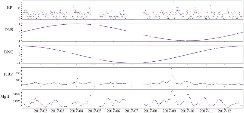
Figure 1. Time series of various geophysical parameters. From top to bottom: Kp, $sin({\omega }_{y}t)$, $cos({\omega }_{y}t)$, f10.7, and MgII time series. ${\omega }_y$ is an annual frequency and $t$ indicates the time index.

The ionogram data was obtained from JRO’s digisonde and filtered using the ARTIST’s quality flags. Times corresponding to geomagnetic events (Kp$>$3) and ionograms with fewer than 10 points were removed from the study. Figure 2 shows the monthly median and median absolute deviation (MAD) of all the ionograms used for training. Notice that the MAD is more prominent near the critical frequencies of both the F and E regions, indicating that the ionograms are more variable and more challenging to model. The usual solar annual and semiannual periodicities can be seen as well.

Figure 2

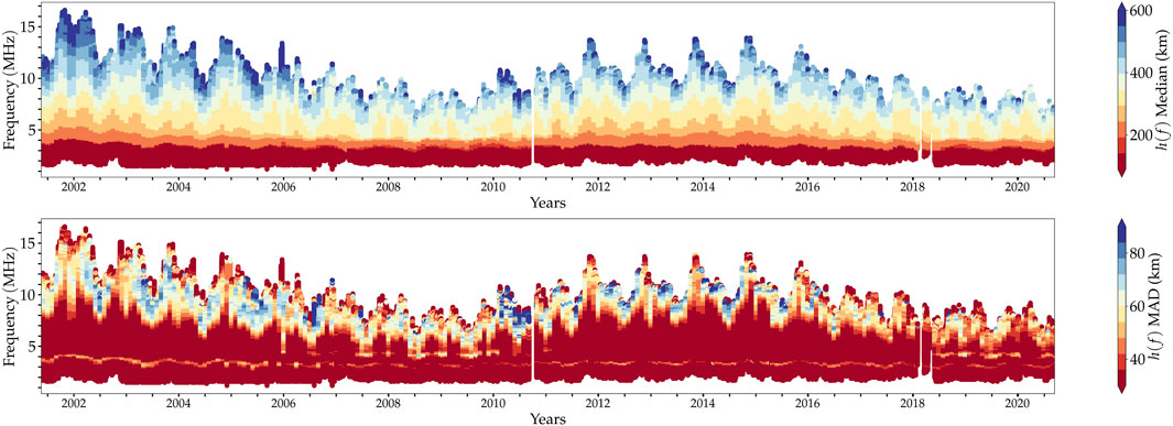
Figure 2. Top: Monthly median of ionograms measured with JRO’s digisonde. The color indicates virtual heights and the vertical axis frequency. Bottom: Median absolute deviation $(\mathrm{M}\mathrm{A}\mathrm{D}(x)=\mathrm{m}\mathrm{e}\mathrm{d}\mathrm{i}\mathrm{a}\mathrm{n}(|x-\mathrm{m}\mathrm{e}\mathrm{d}\mathrm{i}\mathrm{a}\mathrm{n}(x)|))$ of the monthly ionograms.

2.2 Ionograms from empirical models: IRI and SAMI2

To evaluate the accuracy of our model, we compared it against two established ionospheric models: IRI and SAMI2. IRI is an empirical model based on extensive observational data, designed to capture the average behavior of the ionosphere (Bilitza et al., 2022). In contrast, SAMI2 is a physics-based model that solves the ionospheric plasma fluid equations, though it simplifies the system to a 2D geometry and is sensitive to initial conditions. Both models are easy to use and are open to the space physics community. We obtained electron densities as discretized profiles of $N$ elements from these models, and using (Equation 1), we estimated the virtual heights via trapezoidal integration with a correction for the reflection height (Reyes, 2017):

$h\left(f\right)={\int }_0^{z_r}dz{n}_g\left(z\right)\approx {\displaystyle \sum _k^{N-2}}\mathrm{\Delta }z\frac{n_g\left(z_k\right)+n_g\left(z_{k+1}\right)}{2}+\frac{2n_g\left(z_{N-1}\right)\mathrm{\Delta }z}{n_g{\left(z_{N-1}\right)}^2-n_g{\left(z_N\right)}^2}(5)$

We define the group refractive index of the O-mode in (Equation 5) as $n_g(z)={(1-80.62\frac{n_e(z)}{f^2})}^{-1/2}$. This method was validated against Gaussian quadrature, showing no significant differences in accuracy.

2.3 Proposed forecasting models and training strategies

We used two NNs to simulate ionograms: one used a regression model to predict virtual heights, and the other predicted the critical frequency. Regression NNs predict continuous values by learning patterns from input data, making them suitable for forecasting virtual heights, as they can model the smooth variations typically observed in ionograms. By comparing a regression and a classification NN for calculating the critical frequency, we found that the latter more often produced lower discrepancies with the data. The training data for the classification NN consisted of virtual height labels 0 when they did not correspond to the critical frequency and 1 when they did. This NN was trained to predict the occurrence of critical frequencies in ionogram curves as a predictor of label 1 based on the structure of each ionogram. We found that a classification NN and a regression NN were often more effective in determining the critical frequency and the virtual heights, respectively.

To optimize the architecture of our neural networks, we employed Optuna (Akiba et al., 2019), an optimization framework based on Python. Optuna automates the search for optimal hyperparameters using a trial-based approach through efficient sampling techniques and pruning algorithms to explore a large search space. For our model, we used Optuna to fine-tune the learning rates, test different activation functions (ReLU and Swish), and determine the optimal number of nodes per layer. The exact architecture of the NNs can vary because the architecture parameters are part of the hyperparameter optimization process. However, most NNs generated through this process have five layers, use the Swish activation function, and an initial learning rate of approximately 10⁻⁴.

We conducted a series of tests to inform the design of our model. For these tests, we used datasets spanning both 1-month and 3-month periods, specifically selecting months corresponding to solstices and equinoxes. Figure 3 shows some predicted ionograms by our model, SAMI2, and IRI, together with real ionograms measured with JRO’s digisonde. The ionograms obtained with IRI have a visible oscillation near the E-to-F region transition, and the ones obtained with SAMI2 seem to underestimate the variation in this same region. The model’s performance was evaluated by forecasting ionograms and $f_o{F}_2$ values and calculating the root mean square errors (RMSE) compared to the real values obtained with the ionosonde. We also compared the RMSE for predictions made using IRI and SAMI2. The results of these comparisons are summarized in Tables 1, 2.

Figure 3

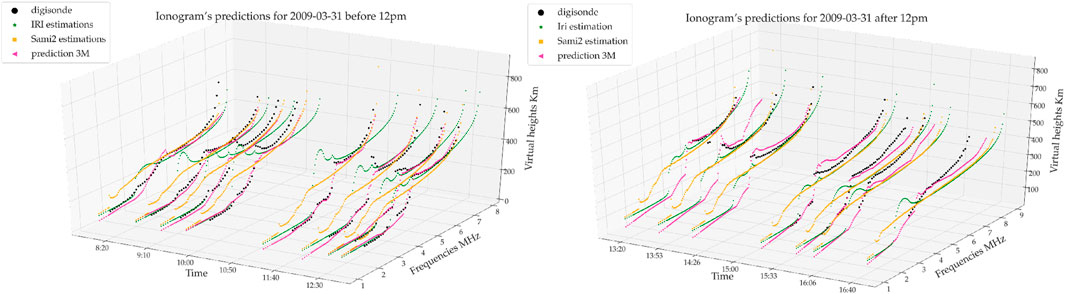
Figure 3. Some sample ionograms for morning (left) and afternoon (right). The ionograms for SAMI2 and IRI were calculated using (Equation 5). The “prediction 3M″ ionograms correspond to the estimated obtained with our first model using 3 months of data.

Table 1

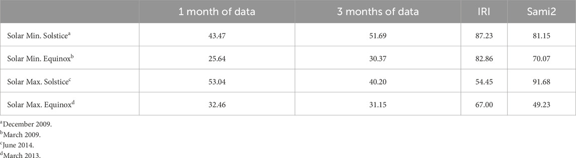
Table 1. RMSE of predicted virtual heights (km).

Table 2

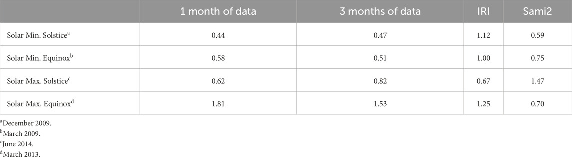
Table 2. RMSE of predicted critical frequencies (MHz).

Across all datasets, our model demonstrated higher accuracy in forecasting ionograms than IRI and SAMI2. The 3-month training dataset did not consistently outperform the 1-month dataset. In most cases, the model trained on 1 month of data yielded better accuracy than the 3-month training. This unexpected result raises questions about the influence of training data size on model performance, which we aim to explore further in future work. Regarding the $f_o{F}_2$ forecasts, our model generally achieved superior accuracy relative to IRI and SAMI2, except for the solar maximum equinox case. Additionally, the 3-month dataset test during the solar maximum solstice produced a forecast that, while less accurate than IRI, still outperformed SAMI2.

These initial results led us to further investigate the influence of the training data time span on the accuracy of our forecasts. To do so, we developed two specialized NNs: IoNNo-C and IoNNo-R.

IoNNo-C was designed to capture long-term behavior and was trained using the complete dataset spanning 18 years. Our goal with IoNNo-C is to model the climatological behavior of the ionosphere and capture finer variabilities that may have been overlooked by empirical models like IRI, which are designed to capture global average behavior. To optimize IoNNo-C, we employed a sliding window technique for hyperparameter tuning. Initially, a set of hyperparameters is selected, and the model is trained on 3 months of data before being evaluated on the following month. This process is repeated over the next 4-month interval, with the average loss function calculated across all windows. After multiple iterations, the set of hyperparameters that results in the lowest average loss function is chosen, ensuring that the model’s parameters do not favor any specific subset of the data.

On the other hand, IoNNo-R was developed for short-term predictions. It is trained using only 3 months of data, with hyperparameters selected to minimize the error for the last week of training data. It is this hyperparameter tuning with recent data that makes this forecasting “shorter-termed.” Furthermore, all the ionograms used in this model were averaged hourly to avoid geophysical noise’s impact in the prediction. This approach aims to maximize the accuracy of immediate, short-term forecasts, providing a complementary perspective to the long-term trends captured by IoNNo-C.

3 Assessing predictions

Each model serves a distinct forecasting needs. IoNNo-R is designed to explore the predictive power of smaller datasets, focusing on short-term, higher-accuracy forecasting. The key feature of IoNNo-R is that its hyperparameters are tuned using data immediately preceding the forecasted period. In contrast, IoNNo-C is built to capture the climatological behavior of the ionosphere over a longer timescale. Because IoNNo-C is trained for the geographic region where the forecasts will be applied, we expect it to provide more accurate predictions than global models that generalize across different locations.

We applied IoNNo-C to predict $f_o{F}_2$ values for the last year of data, which had been extracted from the training set. Furthermore, we trained IoNNo-C with a regression and a classification NN for the critical frequency prediction for comparison. On the top of Figure 4 we can see the smoothed digisonde values (dashed pink line), IRI predictions (dashed blue line), and IoNNo-C predictions (continuous red and gray lines for the regression and classification NN, respectively). From this figure, we observe that IRI systematically overestimates $f_o{F}_2$ values from May to December. In the plot below, we compare the absolute errors of IoNNo-C (red and gray squares for the regression and classification NN, respectively) and IRI (blue triangles). The binary classification version of IoNNo-C achieves slightly better accuracy than its regression counterpart. Moreover, the average improvement of IoNNo-C over IRI is approximately 1 MHz, with IRI exhibiting more extreme outliers.

Figure 4

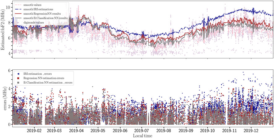
Figure 4. Top: The points in the background correspond to the digisonde data and the models’ estimates. The lines were obtained by smoothing the direct outputs for better visualization. Bottom: The absolute errors for critical frequency estimates of both IRI and IoNNo-C.

For shorter-term predictions, we utilized IoNNo-R. Based on the results with IoNNo-C, we decided to use a classification NN for the virtual height forecasting in IoNNo-C. Figure 5 demonstrates IoNNo-R’s performance in predicting $f_o{F}_2$ compared to IRI from July to September 2019. In the top plot, the digisonde values are marked with light red circles, while the IRI and IoNNo-R predictions are indicated with blue triangles and red squares, respectively. IRI’s systematic overestimation of $f_o{F}_2$ compared to the digisonde measurements is still visible in this shorter time range. Although IoNNo-R predictions are closer to the actual values, a systematic shift relative to the digisonde’s values is still noticeable, particularly in the first half of the time range. Nevertheless, IoNNo-R shows an average $f_o{F}_2$ error improvement of around 1 MHz compared to IRI, matching the improvement seen in IoNNo-C.

Figure 5

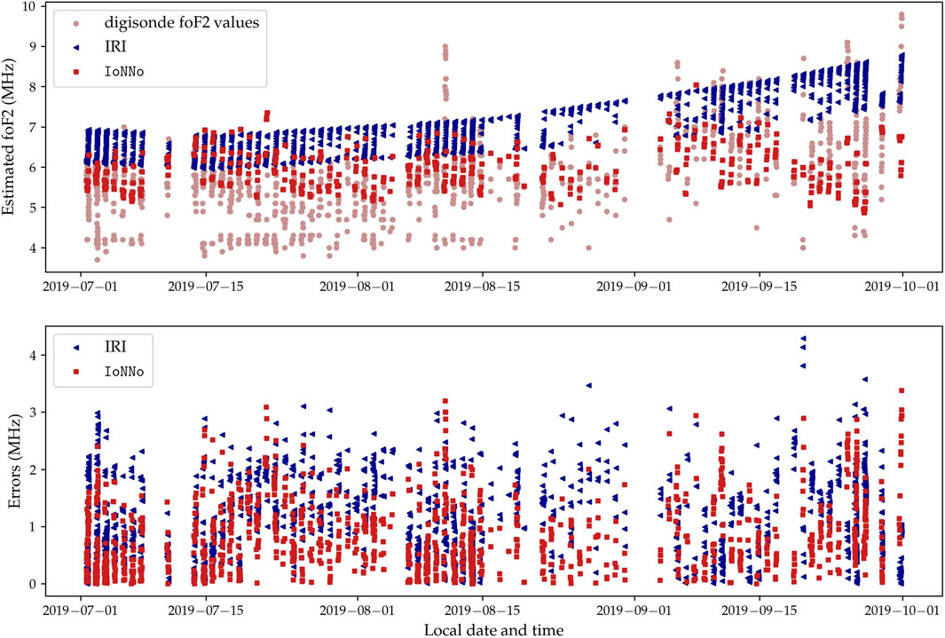
Figure 5. Top: The purple and red triangles and light-blue squares correspond to the digisonde measurements, IoNNo-R predictions, and IRI estimates, respectively. Bottom: The absolute errors for critical frequency estimates of both IRI and IoNNo-R.

Figure 6 analyzes the absolute error statistics for ionogram predictions made by IoNNo-R over the same time interval shown in Figure 5. The figure depicts the distribution of errors, where each box spans the first to third quartiles, with an orange line indicating the median. The whiskers extend up to 1.5 times the interquartile range, and any outliers beyond this range are plotted individually. The top and bottom plots represent morning and afternoon ionograms, respectively. In both cases, the model’s accuracy noticeably decreases as it approaches critical frequencies. However, the afternoon ionograms show significantly less precision, with a greater number of outliers across all frequencies, and higher variability at the upper frequency range.

Figure 6

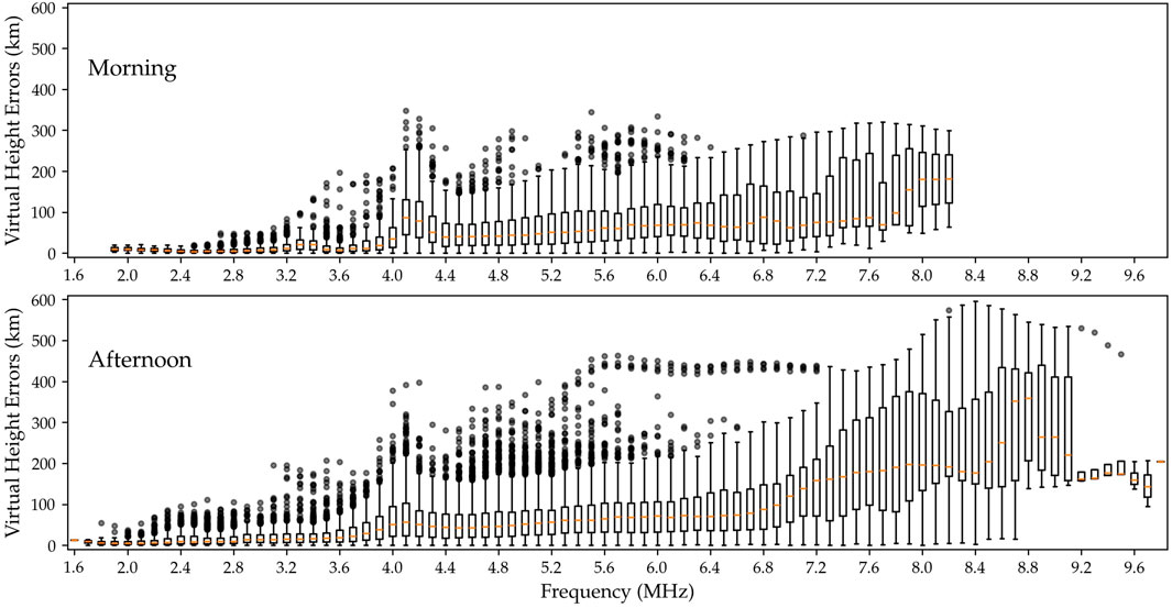
Figure 6. Statistics of virtual height absolute errors of IoNNo-R compared to the digisonde’s ionograms for the same times shown in Figure 5. Each box extends from the first quartile to the third quartile of the virtual heights for each frequency, with a line at the median. The whiskers extend from the box sides to the farthest virtual height lying within 1.5× the inter-quartile range. Points outside the whiskers are indicated independently with gray dots. The top and bottom plots indicate the morning and afternoon ionograms, respectively.

Our analysis has several limitations and shortcomings that need to be acknowledged. First, the accuracy of our comparisons between our models and IRI and SAMI2 relies on the assumption that the ionograms we used are close to the correct values. Although we filtered out ionograms with low-quality flags, our results still depend on the precision of this labeling process. Additionally, our approximation for the virtual height, as expressed in Equation 1, is valid only when the ionosphere is perfectly stratified. This limits its applicability in cases where horizontal gradients are significant, meaning that our model may not fully capture the complexities of certain ionospheric conditions. Finally, the number of samples used to calculate the ionograms using Equation 5) will affect the final form of the virtual height profile. Nevertheless, our numerical tests suggest that the number of points is well within the limit for which the ionogram’s numerical error is smaller than the absolute error of our model predictions.

Moreover, while our models demonstrate promising results, further experiments are necessary to optimize hyperparameters not yet considered in our current framework and optimize the ones we consider in larger parameter spaces. Another limitation is that our models, in their current form, do not incorporate previous information on the ionospheric state. This means that they can not capture temporal dependencies or short-term fluctuations. To address this, we are currently exploring the use of recurrent neural networks that can learn from the time evolution of $f_0{F}_2$ and virtual heights, potentially enhancing the models’ ability to forecast rapidly changing conditions (Hu and Zhang, 2018).

Finally, smoothing the ionograms before training could help remove transient variability. By reducing this variability, we anticipate that our models’ accuracy could improve, providing more reliable forecasts in a broader range of scenarios.

4 Parameter periodicity and predictive power

Our results suggest that even relatively small data sets can be used to train NNs that can match and even outperform IRI and SAMI2 in predicting ionograms and $f_o{f}_2$. Even though this might sound surprising at first, after inspection, we think this should be expected because of the periodic nature of the dominant drivers of the system. For instance, (Wang et al., 2011), analyzed $N_m{F}_2$ time series from ionosondes at different geographical locations and found that the dominant periodicities were consistent with known geophysical and heliophysical periodic forcing.

We can illustrate this by analyzing the periodicity in representative ionosonde parameters. Figure 7 shows a time series of the parameter h’F and its corresponding periodogram. The analysis was done using the Lomb-Scargle method, which is usually recommended over Fourier transforms when gaps are present in the data (VanderPlas, 2018). The h’F parameter captures the virtual height of the bottom of the F region, which is a good proxy for ionogram variability. The red dots in the periodogram indicate the frequency components well above the amplitude that can be assigned to random fluctuations. Notice how the red dots cluster around several well-defined peaks at the diurnal and semidiurnal periods with amplitudes much larger than the smaller components.

Figure 7

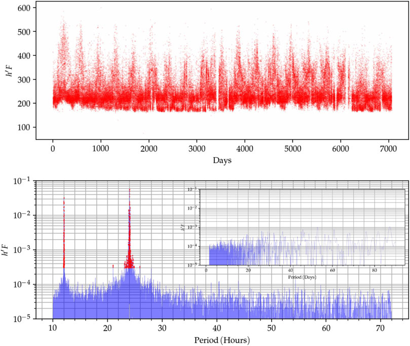
Figure 7. Top: Time series of the h′F parameter. Bottom: Periodograms of h′F up to periods of 70 hours, where the red dots indicate amplitudes significantly larger than expected by white noise. Within the hour-scale periodogram there is a smaller one showing a day-scale periodogram.

The spectral analysis of h’F shows that most of the energy is encapsulated to a few modes. Therefore, we might improve our forecasting efficiency by focusing on predicting the evolution of only the dominant modes using standard time series methods. Nevertheless, it should be considered that given their simplicity of usage current implementation of NNs are still a great forecasting alternative even when its possible to use a sparse representation. Moreover, the NNs have the advantage of possibly capturing nonlinear interactions, which are difficult to include in standard time series models. However, there are currently modeling approaches that are able to exploit the sparse representation of periodic time series and the versatility of NN (Triebe et al., 2021).

5 Conclusion

This study leveraged nearly 2 decades of digisonde data to train NNs for ionogram prediction. Initial small-scale tests on months of equinoxes and solstices indicated that a simple NN could outperform ionogram predictions generated by established models like IRI and SAMI2 in certain situations. We developed two models with distinct datasets and training strategies based on these results. IoNNo-C was trained on the complete dataset, with its hyperparameters tuned to avoid favoring any subset of the data. In contrast, IoNNo-R was trained on only 3 months of data, with hyperparameters specifically optimized to fit the last segment of the training period to improve short-term forecasts.

Our findings show that IoNNo-C consistently produced more accurate $f_o{F}_2$ estimates over a full year of predictions, outperforming IRI. Similarly, IoNNo-R also surpassed IRI’s $f_o{F}_2$ predictions for the studied time intervals, though we observed that the accuracy of ionogram predictions declined at higher frequencies.

Improving short-term ionogram forecasts is crucial before attempting to train a NN to derive electron densities directly from ionograms. However, our results suggest that even short-term datasets may be sufficient for producing accurate ionogram forecasts. We argued that this could be because the dominant periodic forces in the ionosphere are well-resolved within 3 months of data, providing enough temporal information to capture key patterns in ionospheric behavior.

Data availability statement

The datasets generated for this study can be found in the repository “Training data for IoNNo model” located at https://doi.org/10.5281/zenodo.13840721.

Author contributions

ER: Conceptualization, Data curation, Formal Analysis, Investigation, Methodology, Project administration, Resources, Software, Supervision, Validation, Visualization, Writing – original draft, Writing – review and editing. JA: Conceptualization, Data curation, Formal Analysis, Investigation, Methodology, Software, Visualization, Writing – review and editing. MM: Conceptualization, Formal Analysis, Supervision, Writing – review and editing.

Funding

The author(s) declare that financial support was received for the research, authorship, and/or publication of this article. MIT staff was partially supported by NSF grant AGS-1952737. The ionosonde data was obtained from Jicamarca’s Radio Observatory database. The Jicamarca Radio Observatory is a facility of the Instituto Geofisíco del Perú operated with support from NSF award AGS-1732209.

Acknowledgments

The authors would like to thank Reynaldo Rojas for his suggestions for the training of the neural networks.

Conflict of interest

The authors declare that the research was conducted in the absence of any commercial or financial relationships that could be construed as a potential conflict of interest.

Generative AI statement

The author(s) declare that no Gen AI was used in the creation of this manuscript.

Publisher’s note

All claims expressed in this article are solely those of the authors and do not necessarily represent those of their affiliated organizations, or those of the publisher, the editors and the reviewers. Any product that may be evaluated in this article, or claim that may be made by its manufacturer, is not guaranteed or endorsed by the publisher.

References

Akiba, T., Sano, S., Yanase, T., Ohta, T., and Koyama, M. (2019). “Optuna,” in Proceedings of the 25th ACM SIGKDD international Conference on knowledge discovery data mining (ACM), 2623–2631. doi:10.1145/3292500.3330701

CrossRef Full Text | Google Scholar

Bilitza, D., Pezzopane, M., Truhlik, V., Altadill, D., Reinisch, B. W., and Pignalberi, A. (2022). The International Reference Ionosphere Model: A Review and Description of an Ionospheric Benchmark. Reviews Geophy. 60, e2022RG000792. doi:10.1029/2022RG0007921

CrossRef Full Text | Google Scholar

Camporeale, E. (2019). The challenge of machine learning in space weather: nowcasting and forecasting. Space weather. 17, 1166–1207. doi:10.1029/2018SW002061

CrossRef Full Text | Google Scholar

Camporeale, E., Wing, S., Johnson, J., Jackman, C. M., and McGranaghan, R. (2018). Space weather in the machine learning era: a multidisciplinary approach. Space weather. 16, 2–4. doi:10.1002/2017SW001775

CrossRef Full Text | Google Scholar

Gowtam, V. S., and Ram, S. T. (2017). An artificial neural network-based ionospheric model to predict nmf2 and hmf2 using long-term data set of formosat-3/cosmic radio occultation observations: preliminary results. J. Geophys. Res. Space Phys. 122 (11), 743–755. doi:10.1002/2017JA024795

CrossRef Full Text | Google Scholar

Hu, A., and Zhang, K. (2018). Using bidirectional long short-term memory method for the height of f2 peak forecasting from ionosonde measurements in the australian region. Remote Sens. 10, 1658. doi:10.3390/rs10101658

CrossRef Full Text | Google Scholar

Kelley, M. C. (2009). The Earth’s Ionosphere: Plasma Physics and Electrodynamics. 2nd Edn. San Diego, CA: Academic Press. Available online at: https://www.elsevier.com/books/the-earths-ionosphere/kelley/978-0-12-088425-4.

Google Scholar

Laštovička, J., and Burešová, D. (2023). Relationships between fof2 and various solar activity proxies. Space weather. 21. doi:10.1029/2022SW003359

CrossRef Full Text | Google Scholar

McGranaghan, R. M. (2024). Complexity heliophysics: a lived and living history of systems and complexity science in heliophysics. Space Sci. Rev. 220, 52. doi:10.1007/s11214-024-01081-2

CrossRef Full Text | Google Scholar

Reyes, P. (2017). Study of waves observed in the equatorial ionospheric valley region using Jicamarca ISR and VIPIR ionosonde (Ph.D. Dissertation). Urbana, Illinois: University of Illinois at Urbana-Champaign. Available online at: http://hdl.handle.net/2142/98349.

Google Scholar

Triebe, O., Hewamalage, H., Pilyugina, P., Laptev, N., Bergmeir, C., and Rajagopal, R. (2021). Neuralprophet: explainable forecasting at scale

Google Scholar

Uwamahoro, J. C., Giday, N. M., Habarulema, J. B., Katamzi-Joseph, Z. T., and Seemala, G. K. (2018). Reconstruction of storm-time total electron content using ionospheric tomography and artificial neural networks: a comparative study over the african region. Radio Sci. 53, 1328–1345. doi:10.1029/2017RS006499

CrossRef Full Text | Google Scholar

VanderPlas, J. T. (2018). Understanding the lomb–scargle periodogram. Astrophysical J. Suppl. Ser. 236, 16. doi:10.3847/1538-4365/aab766

CrossRef Full Text | Google Scholar

Wang, W., Lei, J., Burns, A. G., Qian, L., Solomon, S. C., Wiltberger, M., et al. (2011). Ionospheric day-to-day variability around the whole heliosphere interval in 2008. Sol. Phys. 274, 457–472. doi:10.1007/s11207-011-9747-0

CrossRef Full Text | Google Scholar