The response of exospheric neutral hydrogen to weak geomagnetic disturbances between June 12 and 29, 2008

Stereoscopic remote sensing observations of terrestrial far ultraviolet (Lyman-α at 121.6 nm) emissions at solar minimum have been used to retrieve the time-dependent response of the exospheric 3-D neutral hydrogen (H) density at radial distances of 3–6 Earth radii (R_e) to weak geomagnetic disturbances. This study includes continuous observations from the Lyman-α detectors (LADs) onboard NASA’s Two-Wide angle Imaging Neutral-atom Spectrometers (TWINS) 1 and 2 satellites between June 12 and 29, 2008, which covers two minor geomagnetic storms (June 15 and 25). For both storms, we derived the 3-D H-density distributions from prior and during-storm data with 12 h time intervals. The inversion is based on our new H-density EXPGRID model and incorporates the effects of Lyman-α absorption within the exosphere and Lyman-α re-emission from Earth’s albedo. We found that the H-density distributions at 3–6 R_e are highly variable. They are correlated and vary in phase with exobase temperatures (from Naval Research Laboratory mass spectrometer and incoherent scatter (NRLMSIS)) during the geomagnetic events. Furthermore, the time dependency and amplitude of the H-density enhancement and the kp index were found to be similar. Because the kp index is assumed to be correlated with the varying size of the plasmasphere, this finding supports theories of physical interaction between the neutral exosphere and the plasmasphere. The disturbances with a significant effect on the neutral H atoms are initiated by a prior increase of the solar wind flow pressure and exobase temperatures (in particular, over the poles). Our time-dependent 3-D results indicate that the H-atom enhancement is not uniformly distributed over the shells. Instead, we found asymmetries (i.e., dawn/dusk near the ecliptic) and temporal evolving zones of regionally strong enhanced H densities. Among the first affected regions after onset are the vicinities of the geotail (at lower distances) and the North Pole (at upper distances). A ∼40% exobase temperature increase (NRLMSIS) at the South Pole on June 15 correlates with a strong H-atom enhancement in the southern hemisphere later this day. Finally, both storms show, at the upper distance, a remarkably delayed enhancement (peak values as late as ∼2 days after onset) of the H atoms density near the sub-solar point (dayside “nose” region).

1 Introduction

Atomic hydrogen (H) is the dominant component of the terrestrial exosphere, which extends from ∼500 km altitude up to several tens of Earth radii (R_e) (Baliukin et al., 2019). In this vast region, exospheric H atoms permanently interact with ambient magnetospheric ions via charge exchange processes, playing a crucial role in their dynamics, especially during geomagnetic storms (Ilie et al., 2013; Krall et al., 2018; Cucho-Padin et al., 2025; Lin et al., 2024). Historically, inner magnetospheric modeling (e.g., ring current, plasmasphere) assumed that exospheric H-density distributions do not vary during the evolution of a storm; however, this statement has been challenged by recent studies based on the observed Lyman-alpha (Ly-α @ 121.6 nm) emission, which is resonantly scattered by H atoms.

The first report of temporal variation of the exospheric Ly-α column brightness during geomagnetic storms was done by Bailey and Gruntman (2013) using radiance data acquired by the Lyman-α detectors (LAD) onboard NASA’s Two-Wide angle Imaging Neutral-atom Spectrometers (TWINS) mission (McComas et al., 2009; Nass et al., 2006). In this study, a parametric estimation method was utilized to determine the atomic H density in the 3–8 R_e region, which in turn was used to calculate and analyze the variability of the total H-atom content in response to geomagnetically active periods that occurred from August to November 2011. They found an enhancement of H densities, which was correlated with the geomagnetic disturbance (Dst) index. Zoennchen et al. (2017) conducted a similar study using TWINS/LAD data for several storms in the 2008–2012 period, spanning solar maximum and minimum conditions. The analysis of radiance measurements, whose impact distance was greater than ∼2R_e altitude (i.e., the optically thin region of Earth’s exosphere), unveiled emission enhancements of 6%–23%. At these altitudes, the column-integrated photon flux along a given line-of-sight (LOS) is highly correlated with the atomic H density owing to its single photon scattering nature; therefore, it was inferred a similar enhancement in exospheric H densities. Furthermore, Kuwabara et al. (2017) reported similar storm-time variations in Ly-α radiance data acquired by the EXtreme ultraviolet spectrosCope for ExosphEric Dynamics (EXCEED) instrument on board the Hisaki satellite. With an acquisition rate of ∼90 min and observation geometry pointing in an antisunward direction with most of the line-of-sight in the optically thin region, they identified abrupt enhancements of up to 10% in the column-integrated Ly-α radiance within a 2–4 h period, possibly related to the rapid inward movement of the plasmapause during storm-time (plasmaspheric density depletion). Cucho-Padin and Waldrop (2019) implemented a robust dynamic tomographic method that used LAD radiance measurements of TWINS2 to estimate the time-dependent, global H-density distributions during the minor geomagnetic storm that occurred on June 15–18, 2008. They reported (1) a significant increase of H densities of ∼25% within the sub-solar point at 3R_e geocentric distance that exhibited high anti-correlation with the Dst index and (2) exospheric upwelling possibly associated with the increase of exobase temperature as well as charge exchange interactions with the plasmasphere. Recently, efforts have been made to analyze this storm using physics-based modeling. Connor et al. (2024) carried out the implementation of a Monte Carlo model that solves the kinetic equation of H atoms, which considers thermal velocities provided by exobase temperatures and the effect of terrestrial gravity to determine escaping and ballistic particle trajectories. This study stated that the increase of H density during the storm has good agreement with the increase of exobase temperature, although no H atoms produced by charge exchange with ambient ions were included in the simulation.

Based on different approaches, inversions of TWINS LAD radiance data observed during stable geomagnetic conditions at solar quiet times into static 3-D H-density models were already done in the past: Bailey and Gruntman (2011); Zoennchen et al. (2015) used a spheric harmonic representation (SHR) density model of order L = 2 (Nass et al., 2006). It basically consists of a (global) radial symmetric H-density term (in the form of a power law function over distance r) multiplied by an angular modulation term (formally known as spheric harmonic representation). Cucho-Padin et al. (2022) presented a high degree of freedom (HDOF) tomographic approach, which allows the estimation of density distributions without the dependence on ad hoc functions. The HDOF method solves an inverse problem y = Lx that linearly correlates background-free Ly-a measurements (y) and hydrogen densities (x) using the maximum A posteriori (MAP) approach. To do so, the HDOF method defines a region of interest as a spherical region that spans radii from 3 R_e to 20 R_e and discretizes it into regular spherical voxels. Then, TWINS/LAD lines-of-sight (LOSs) are intersected with the voxels, and the length of such an intersection is stored in the observation matrix L. Thus, y is a [Mx1] vector, where M is the number of measurements; x is a [Nx1] vector, where N is the number of spherical voxels in the domain; and L is a [M x N] matrix. Because TWINS 3D locations, LAD’s LOS direction, and the size of the voxels are provided, L can be implemented. Finally, when a set of observation and their values in Rayleighs are provided, we can estimate x using the robust MAP technique, which considers the probability distribution of the signals (i.e., Poisson distribution in the measurements) [see more details in Cucho-Padin et al. (2022)]. In Zoennchen et al. (2024), the static 3-D inversion results of an improved SHR model (order L = 3) and of the HDOF approach are both compared with the usage of TWINS/LAD data from quiet summer solstice days during solar minimum (2008) and maximum (2013 and 2015).

In this work, we conduct a thorough analysis of the temporal evolution of the 3-D exospheric density distributions during two minor geomagnetic storms using our novel 3-D H-density method, EXPGRID. The present work differs from that shown in Cucho-Padin and Waldrop (2019) not only in the amount of analyzed data (17 days) and the applied estimation technique but also in a significantly improved stereoscopic coverage (by incorporating data from both TWINS spacecraft) and in additional correction factors incorporated in the analysis, such as (1) the self-consistent Ly-α absorption within the exosphere, (2) the re-emission of Ly- α radiance from Earth’s albedo, (3) a temperature-dependent cross section of the photon-atom interaction, and (4) the use of data acquired by the two LADs on each TWINS satellite. We reconstruct the dynamic exosphere from TWINS/LAD measurements acquired during the two storms on June 15–19 and June 25–29 in 2008. Section 2 describes the LOS inversion approach, the new 3-D H-density model EXPGRID, the geomagnetic storm events, and the LAD data selection used in this study. Section 3 shows the results of the reconstructions of the exosphere. Section 4 presents the conclusions of this study and the outlook for future work.

2 Materials and methods

2.1 Approach and LOS corrections

In the optically thin regime of the terrestrial exosphere (beyond 3 R_e geocentric distance), the atomic H density is low enough such that the scattering with solar Lyman-alpha (Ly-α) photons is assumed to occur only once. This condition yields a linear relationship between the local exospheric density $n\left(S\right)$ [atoms/cm³] and the exospheric backscattered Lyman-α column brightness $B$ in Rayleighs [1 (R) = 10⁶ photons ($4\pi ·{cm}^2·s·sr$)⁻¹] along a line-of-sight $S$ given by the following formula (Østgaard et al., 2003):

$B=4\pi I=\frac{g^{*}}{{10}^6}{\int }_0^{s_{\mathit{max}}}n\left(S\right)\epsilon \left(S\right)\gamma \left(S\right)\mathrm{\Psi }\left(\alpha \left(S\right)\right)dS,(1)$

where $\epsilon \left(S\right)$ represents the local Earth albedo correction term (unitless), γ($S$) is the local loss term of photons on its way back to the detector (unitless), and Ψ(α($S$)) is the local intensity correction due to the dependence of the scattering efficiency on the angle α between the line-of-sight S and the incident solar photon (Brandt and Chamberlain, 1959). The scattering rate (or g-factor) g* [photons/atom/sec] is the product of the scattering cross-section σ [cm²], and the effective solar Lyman-α flux at line center F_eff [photons/cm²/s], and the superindex * indicates its adjustment from 1 AU to the actual Earth-Sun distance.

The solar Lyman-α at line-center flux, F_eff, can be derived from the total solar Lyman-α flux [which is obtained by the Solar EUV Experiment (SEE) onboard NASA’s Thermosphere Ionosphere Mesosphere Energetics and Dynamics (TIMED) Mission] using the relation given by Emerich et al. (2005).

In a real case scenario, an observation of the terrestrial exosphere by a Ly-α photometric detector along the LOS $S$ will contain additional background information from the Lyman-α glow of the interplanetary H atoms (also known as IPH-background), which must be subtracted. In this work, we used a hot model of the interplanetary H-density distribution (Fahr, 1971; Thomas, 1978) to calculate all sky maps of the Lyman-α background flux daily. The model parameters and assumptions used are detailed as described by Zoennchen et al. (2015).

In our study, the Earth’s albedo correction term $\epsilon \left(S\right)$ has two additive components. The first is the backscattered Lyman-α re-emission from the lower (optically thick) exospheric region with high H densities at the dayside, which acts as a secondary source of Lyman-α. The second is the solar Ly- α flux that is absorbed and re-emitted as it transits within the exosphere, resulting in a reduced photon flux reaching the exospheric night side. In addition, our emission model Equation 1 includes a third correction term, $\gamma \left(S\right)$, that accounts for a loss of scattered photons on their way from the position of origin to the detector (along the inverse LOS direction). The explicit formulation and the use of these three correction terms are described in detail by Zoennchen et al. (2024).

2.2 Reconstruction of the exospheric 3-D H density distribution

We used a new model approach referred to as EXPGRID in this analysis to retrieve the exospheric 3-D H-density distribution.

The EXPGRID model uses spherical geocentric solar ecliptic (GSE) coordinates, and it is based on three different reference shells at radial distances of 3.125 R_e, 4.125 R_e, and 5.125 R_e. These three radii are distributed over the optically thin range and are best observed by TWINS/LADs. Each shell is discretized into 104 angular segments (in total, 312 segments for all three shells). Each segment stores the H-density value at its distance and angular position.

Different from a usual spherical grid, the EXPGRID segments on a shell are designed to all have a nearly constant physical length (km) in longitude. This is not the case in a usual spherical grid, where the longitudinal physical length of a segment decreases with cos (lat) (lat = latitude). The effect of the shrinking longitudinal segment size is caused by the decreasing circumference of a latitudinal circle at higher latitudes. Because all meridians on a shell have equal lengths, the latitudinal physical lengths of all segments are equal naturally.

On a given shell, the segments used by EXPGRID all have a nearly constant longitudinal and latitudinal physical length (at their center positions) of approximately 1/18 of the shell circumference. As a result, all segments cover nearly the same fraction of the shell surface. In latitude, this physical length corresponds, as usual, to a fixed angular latitudinal size of ∼20° for every segment. To keep the longitudinal physical length nearly constant, the number of segments per latitudinal circle $N_{seg}\left(lat\right)$ must be reduced with latitude,

$N_{seg}\left(lat\right)=\mathit{int}\left[N_{0°}·\cos \left(lat\right)\right](2)$

where $N_{0°}$ = 18 is the number of segments at the ecliptic latitudinal circle (lat = 0°) with a 20° longitudinal angular size. The reduction of the segment number on all other latitudinal circles Equation 2 is equivalent to an expansion of the segment longitudinal angular size with latitude. According to Equation 2, the longitudinal physical length of all segments is nearly (and not exactly) constant because the segment number must be in whole numbers (integer) on each latitudinal circle. In Figure 1, the angular grid used in the EXPGRID H-density model is shown together with the segment number per latitudinal circle (see blue numbers in brackets).

Figure 1

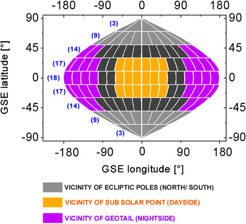
Figure 1. Illustration of the grid used in the EXPGRID H-density model. Shown is the distribution of the angular segments over a shell. Blue numbers in brackets indicate the segment count of the corresponding latitudinal circle. The maximal segment count on a latitudinal circle is 18 at the ecliptic circle (GSE lat = 0°). For higher latitudes, this count decreases to preserve a similar longitudinal physical length (measured in the segment’s latitudinal middle) of all segments on the shell. The total number of segments per shell is 104 (36% less than a regular angular 20° × 20° grid). The four different regions in the vicinities of the ecliptic poles, the sub-solar point, and the geotail are schematically marked with different colors and labeled below the grid image.

One motivation to use this grid inside the EXPGRID model is the reduction of the total number of segments (also identified as model coefficients) by 36% compared to a regular spherical 20° × 20° grid, which significantly improves the performance of our least squares fitting process.

The segments of the same angular position $\left({\phi }_i,{\vartheta }_j\right)$ are radially connected across the three shells by an individual exponential function with the form:

$n_H{\left(r\right)}_{{\phi }_i,{\vartheta }_j}=\exp \left(a_{{\phi }_i,{\vartheta }_j}+\frac{b_{{\phi }_i,{\vartheta }_j}}{r}+c_{{\phi }_i,{\vartheta }_j}·\ln \left(r\right)\right)(3)$

This function consists of the three segment-specific parameters, $a_{{\phi }_i,{\vartheta }_j}$, $b_{{\phi }_i,{\vartheta }_j}$ and $c_{{\phi }_i,{\vartheta }_j}$, which are fully constrained by solving the systems of equations using the three $n_H{\left(r_{shell1,2,3}\right)}_{{\phi }_i,{\vartheta }_j}$ H-density values (=model coefficients) from the radial connected segments. Based on that constraint function, the radial H-density profile at any given distance r for the angular position $\left({\phi }_i,{\vartheta }_j\right)$ can be calculated.

Summarized, the EXPGRID model provides an individual radial exponential function (of type as shown in Equation 3) for each angular grid segment $\left({\phi }_i,{\vartheta }_j\right)$. These functions are constrained by the H densities of the corresponding segments at the same $\left({\phi }_i,{\vartheta }_j\right)$ positions on the three reference shells. The specific form of the exponential function (also known as the vapor pressure function) was chosen because it fits very well the different radial profiles from varying angular positions of a 3-D H-density cube calculated with the HDOF model approach for the solar quiet day of June 12, 2008 (see Zoennchen et al., 2024). The H densities of neighboring segments are linearly interpolated to retrieve H densities at any given angular position.

Within the inversion procedure, we used a least square fit to minimize the difference between observed and modeled LOS column brightness, together with an additional regularization term, to enforce a solution with optimal smoothness. The methodology with implemented regularization is extensively described by Zoennchen et al. (2024); see Section 2.2.1 therein.

Regions of particular interest, like the vicinities of the sub-solar point, the geotail, and the two ecliptic poles, are marked with different colors in Figure 1.

2.3 Solar and geomagnetic conditions

The entire period of selected data from June 12 to 29, 2008, represents the H geocorona near the summer solstice in the solar minimum. The solar total Lyman-α flux is nearly stable on a very low level. It slowly varies within a ∼2% range between 3.46 × 10¹¹ photons/cm²/s and 3.61 × 10¹¹ photons/cm²/s.

Within this period, two major events of geomagnetic disturbance with a significant impact on the exospheric H densities were found (see marked as Event1 and Event2 in Figure 2). In addition to these major events, there are two smaller sub-events (marked as Sub1 and Sub2 in Figure 2), which are also followed by minor peaks of higher H densities at 3–6 R_e [see Figure 2H].

Figure 2

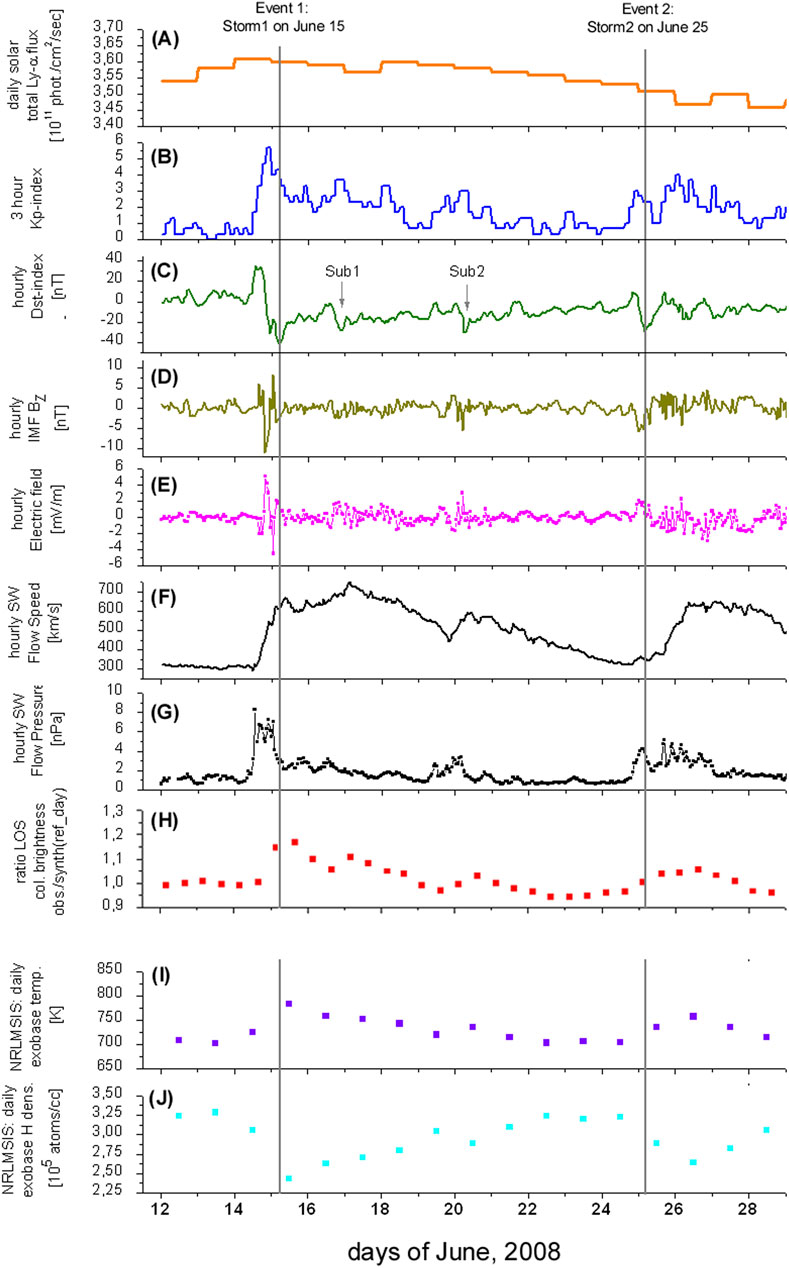
Figure 2. (A–G) show solar and geomagnetic conditions for the period June 12–29, 2008 as the solar total Lyman-α flux [daily, (A)], the kp index [3 hourly, (B)], the Dst index [hourly, (C)], the IMF Bz component in GSM [hourly (D)], the electric field calculated from plasma flow speed and IMF Bz [hourly, (E)], the SW Flow Speed [hourly, (F)] and the SW Flow pressure [hourly, (G)]: While the total solar Lyman-α flux is stable within 2%, the kp and Dst indices and the SWFP vary significantly and indicate the geomagnetic disturbance. The two major disturbances (analyzed in 3-D) are minor storms and are marked as Event1 and Event2 with vertical gray lines at their minimum Dst indices. Before the two events, there is a rapid enhancement of the SW Flow pressure (G), which is immediately followed by perturbations of the magnetic field (D) and the convection electric field (E). The latter is a driver for enhanced particle precipitation in the cusp and auroral regions; also marked are two minor disturbance events, sub1 and sub2. All four marked events have geomagnetic disturbance levels much smaller than strong events at solar maximum. Nevertheless, they are able to cause observable enhancements of the H exosphere above 3 R_e [see (H)]. (H) shows the timeline of the LOS column brightness ratio (averaged per orbit) of TWINS2 LAD observed values versus synthetic values using the H-density model of the quiet reference day, June 13. Ratio values > 1, which are visible during the events, indicate that above 3 R_e, the current number of exospheric H atoms is higher during geomagnetic disturbances than on the quiet reference day. (I, J) present for the same period the timelines for temperature and the H-density at the exobase (daily averaged, provided by NRLMSIS). The time dependencies of exobase temperature and H-density ratio above 3 R_e [see (H)] are positively correlated and very similar. The exobase H density varies inversely to that: its time dependency is anti-correlated to the H-density ratio above 3 R_e.

The timelines of the geomagnetic parameters shown in Figure 2A–G have similarities and also characteristic differences for the two major events:

The geomagnetic similarities are:

• The earliest observed sign of variability in both events is a simultaneous and significant (positive) enhancement of solar wind flow pressure (SWFP), kp-, and Dst index. This enhancement starts several hours before the Dst index reaches its minimum value, specifically ∼16 h for Event1 and ∼13 h for Event2, respectively.

• After the Dst index reached its minimum (in the morning at ∼4–5 a.m.), both storms entered a phase of recovery for several days, where disturbance levels of the geomagnetic parameters slowly returned to zero.

• During both storms, there is an increase of the solar wind flow speed (see Figure 2F) from ∼300 km/s up to 600–700 km/s as well as evident perturbations of the magnetic field (interplanetary magnetic field (IMF) B_z) and the electric field (see Figures 2D, E).

• During the events, the variations of the SWFP and the kp index are very similar in relative amplitude enhancements versus time. Even minor sub-peaks in the SWFP can be recognized in the kp index (see Figures 2B, G).

The geomagnetic differences are:

• Event1 has an initial SWFP enhancement by a factor of 6–7 that starts at noon on June 14 with a sharp increase. It lasts for approximately 12 h and is constantly high during that time. A higher SWFP is related to a higher compression of the Earth’s magnetosphere. Larger values of the kp index are associated with a movement of the plasmapause closer to Earth (Moldwin et al., 2002).

• In comparison, Event2 has a smaller initial SWFP peak by a factor of ∼4, which lasts for 4 h only. In addition to this primary peak, Event2 has a secondary phase of pressure enhancement (from the afternoon of June 25 until the end of June 26) with an even higher amplitude than the primary. It consists of a series of single short-time pressure waves with durations of several hours each.

• The range of the Dst index drop (from its prior positive to the negative peak) is approximately twice as high for Event1 [35 – (−41) = 76 (nT)] as Event2 [9 – (−29) = 38 (nT)]. The maximum kp index value of Event1 is 5.7, which is higher than that of Event2 by a factor of ∼1.4.

• The perturbations of the magnetic field IMF B_z and the electric field, respectively, are different for both storms: Event1 shows a rapid fall of IMF Bz to −11 [nT] (southward) ∼11 h before the Dst index minimum, followed by an increase and turn in orientation to +8 [nT] (northward) until June 15, 1 a.m. This feature highly correlates in time with the sudden increase of the SWFP. In contrast, Event2 shows a much smaller and more diffuse IMF B_z perturbation. It started at 8 p.m. on June 24 with a fall to −5.7 [nT] at midnight and turned back to northward +3 [nT] at 9 a.m. on June 25. During the next 3 days, it appeared continuously perturbed on a low scale [<|4| (nT)]. For both events, the electric field is similarly but inversely perturbed as the IMF B_z. (see Figures 2D, E, G).

• The increase of the solar wind flow speed began at different times with respect to the Dst index minimum: ∼14 h prior to Event1 and ∼4 h after Event2 (see Figure 2F).

• For both events, there is a nearly synchronized increase in the temperatures at the exobase (based on the NRLMSIS model). This temperature increase is larger (in particular over the poles) for Event1 than Event2 (see Section 3.2.3).

Due to the larger variation of the described geomagnetic parameters, Event1 is expected to have a higher impact on the exosphere than Event2. This was finally confirmed by the LAD observations.

For geomagnetic activity classification of the discussed events, we lean on the G-scale from NOAA (see https://www.swpc.noaa.gov/noaa-scales-explanation), which is based on the maximum kp-level during an event. Regarding this G-scale, Event1 can be considered a minor storm (G1). Event2 is below storm level G1 in the NOAA G-scale but is very close to the border. Similar to Event1, it also comes with storm-like characteristics as the significant increase of the Solar Wind (SW) flow speed and flow pressure, respectively. Therefore, we want to consider Event 2 as a minor storm in this work. Additionally, we use the terminology “weak” as a grouping label for events with kp <6 (meaning lower than the “moderate storm” level), which is the case for all events discussed here.

The two sub-events, Sub1 and Sub2 (both G0), are considered weak disturbances below storm level for several reasons: Compared to the two storm events, the sub-events have lower maximal kp values (3.7 and 3) together with significantly smaller SW flow pressure peaks. In addition, the perturbation of the IMF B_z is relatively small. Finally, there is no large increase in the SW flow speed during Sub1 and Sub2, as is the case for the two minor storms. Both sub-events started on still-increased SW flow speed levels, which are substantially higher than the ∼300 km/s prior to the first storm. Therefore, the first minor storm and the two sub-events seem to be part of the same solar wind event (as a type of co-rotating interaction regions (CIR)) of enhanced flow speed. For differences between CIR-driven storms and CME-driven storms, see Borovsky and Denton (2006).

Even if the strength of the geomagnetic disturbance of all four events is low compared to strong storms during solar maximum [with a Dst index minimum below - 200 (nT), that is, on May 04, 1998 (Khazanov et al., 2004)], they can cause observable variations of the neutral H geocorona at 3–6 R_e.

2.4 Selection of TWINS LAD data

Selected LAD data of both TWINS spacecraft were analyzed between June 12 and 29, 2008. This period contains LAD observations from the very first days of the TWINS mission. TWINS1 and 2 are situated longitudinally (GSE) on the dawn and the dusk side at an angle ∼20° from the noon-midnight meridian. There is a slow move (∼1°/day) clockwise towards the dawn side in GSE longitude.

The LOSs are limited to those impact distances ≥3.0 R_e in order to keep the calculations inside the optically thin regime. Further removed are observations contaminated by scattered sunlight (LOS–Sun-angles ≤90°) or with an intersection of regions near the shadow or the Earth’s penumbra (LOSs with tangent point radial distances ≤3 R_e from the negative GSE X-axis). We tracked UV-bright stars [list of stars taken from Snow et al. (2013)] and removed all LOS crossing the 8° angular region around a star from that list.

Because both TWINS spacecraft were operational at this time, the spatial and temporal coverage of the Earth exosphere represent the best data deliverable by observations from this mission and allow for a good stereoscopic view in Lyman-α. In addition, the measurement quality in terms of noise and stability of LADs sensitivity is best compared to later years because the sensors are not particularly exhausted at this early phase of the mission.

Nevertheless, there is an exception from stability regarding sensor LAD2 of TWINS2. It shows a measurable sensitivity decline for a so far unknown reason. During the analyzed period, the UV-bright star α Cru was observed with this LAD sensor. These observations with LOS directions inside a ∼5° circle around the star were used to calculate the time-dependent LAD sensitivity from the decreasing stellar peak values (see Figure 3). Hereby is the ratio of the observed current versus the initial stellar peak Lyman-α count rate equal to the ratio of the current versus the initial LAD sensitivity. With knowledge of the LAD sensitivity f_{cal, init} and the stellar peak count rate at the initial time, the current LAD sensitivity at a given time t f_cal(t) can be calculated based on the stellar peak count rate at t following Equation 4:

$f_{cal}\left(t\right)=f_{cal,init}·\frac{{Ly}_{\alpha }countratestellarpeak\left(t\right)}{{Ly}_{\alpha }countratestellarpeak\left(t_{init}\right)}(4)$

Figure 3

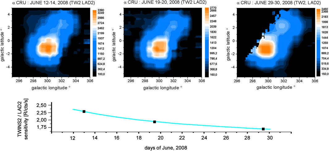
Figure 3. Upper row: Lyman-α observation of the star α Cru by TWINS2 LAD2 at three different times between June 12 and 30, 2008. The continuous drop of the observed stellar peak Lyman-α count rate is equivalent to a reduction of the sensor’s sensitivity to 73% at the end of the period. The reason for that sensitivity reduction is so far unknown. Lower row: The time-dependent sensitivity of that sensor was adapted by a polynomial function.

Figure 3 shows the peak count rate of star α Cru observed by TWINS2 LAD2 continuously falling from its initial value of 3,380 on June 12–14 to 2,460 [counts/0.67 s] on June 29–30. The effect must be interpreted as a continuous loss of this sensor’s sensitivity down to ∼73% of its initial value. The method is described in detail with the usage of multiple stars for all four LAD sensors by Zoennchen et al. (2024). In addition, the calibration error of approximately 5% and the initial sensitivity values in [counts/sec/Rayleigh] of all four LADs from 12 June 2008 can be found in Section 2.5 and Table 2 of Zoennchen et al. (2024).

For the 3-D study of the two major events, we analyzed LAD data from both TWINS of June 13–19 (Event1) and June 24–29 (Event2). From the asynchronous operational hours of the TWINS 1 and 2 satellites, the best time overlap between them was found in the 12 h intervals at 0 a.m.–12 p.m., 5 a.m.–5 p.m., 12 p.m.–0 a.m. (next day), and 5 p.m.–5 a.m. (next day). Another major criterion for being selected as a usable interval is the existence of a sufficient number of observations from all four LAD sensors. The time intervals finally selected for the 3-D H-density inversions are shown together with the inversion results in Figures 4, 5.

Figure 4

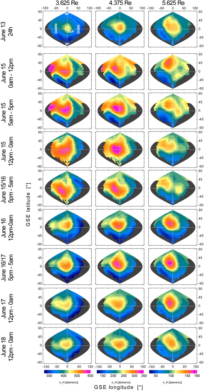
Figure 4. H-density maps from the 3-D inversion of Storm1 (rows 2–9, 12 h intervals) and June 13 (first row, 24 h interval) as a quiet day prior to the storm for comparison. Shown are the H density distributions in [atoms per cc] at the lower (3.6 R_e), middle (4.4 R_e), and upper distance (5.6 R_e). Remarkable are the significant H-density enhancements during the first ∼1.5 days (rows 2–5), which are mostly located on the dawn side at lower and middle distances. Interestingly, there is a delayed H enhancement of the dayside nose (near the SSP) at the upper distance (right column), which reaches its maximum H density ∼2 days after the storm onset. Possible reasons for that phenomenon could be a low velocity (∼70 m/s) transportation of H atoms up to that distance and/or the force of the solar radiation pressure, which focuses the different orbital planes of orbiting H atoms into the GSE XZ-plane above the SSP. Gray areas represent regions that are not covered by LOS observations with Earth tangent points between 3 and 6 R_e.

Figure 5

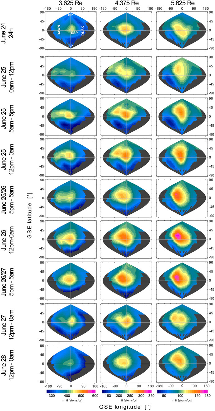
Figure 5. H-density maps from the 3-D inversion of Storm2 (rows 2–9, 12 h intervals) and June 24 (first row, 24 h interval) as the quiet day prior to the storm for comparison. The H density distributions in [atoms per cc] at the lower (3.6 R_e), middle (4.4 R_e), and upper distance (5.6 R_e) are also shown with the same color-coding scale used in Figure 4. The H-density enhancements caused by Storm2 are clearly smaller than those of Storm1 (Figure 4). At the lower distance, the most significant is a band-like structure of higher H-density from the SSP to the dawn side near the ecliptic. More enhanced dawn-side H densities are a feature common to both analyzed storms; also visible at the upper distance during Storm2 are the by-∼2 days-delayed (with respect to the storm’s onset) peaks of maximal dayside H-density near the SSP. Gray areas represent regions that are not covered by LOS observations with Earth tangent points between 3 and 6 R_e.

In order to identify storm-time global variations of the exosphere using column-integrated Ly-$\alpha$ emissions, we estimated the 3-D H-density model from data acquired by TWINS/LADs on June 13, which were used as a reference. Then, we estimated the LOS emission during the quiet time (June 13) and the storm-time period (June 12–29) for the TWINS2/LADs instruments and created the ratio LOS $intensit{y}_{storm\_time}$/LOS $intensit{y}_{quiet\_time}$, which is shown in Figure 2H.

3 Results

3.1 Highly variable H densities at 3–6 R_e

During the analyzed period at solar minimum 2008, our study revealed that the exospheric H densities at 3–6 R_e respond mostly with an enhancement to minor storms. Interestingly, this is also the case for the two sub-disturbances (marked as Sub1 and Sub2 in Figure 2), which were very weak compared to the minor storms. The exospheric response can be seen in Figure 2H from the variation of the ratio between LOS observed column brightness versus the calculated value based on the quiet 3-D H-density model of June 13.

Because those weak geomagnetic disturbances are relatively frequent, our result implies that the exospheric H-density distribution at 3–6 R_e can be considered highly variable. At these distances, the assumption of a static quiet H geocorona seems to match only during a very limited number of short periods (even at solar minimum).

Figure 2 shows a very similar time dependency of the relative variation of the H-density [panel (H)] and the kp index [panel (B)], which suggests a physical connection between the two. The kp index is correlated to the size of the plasmapause (Moldwin et al., 2002). The peak height of the H-density enhancement [panel (H)] is correlated with the strength of the perturbation of the IMF B_z, [panel (D)] and the electric field [panel (E)]. IMF B_z and electric field are interconnected with the peak height of the SW flow pressure increase [panel (G)] (Nilam et al., 2020).

3.2 3-D inversion results of Event1 and Event2

For Event1 and Event2 (see Figure 2), our 3-D inversions of the H density (based on the EXPGRID model) were derived using the 12-h intervals explicitly, as shown in Figures 4, 5 (vertically at the left side) between the event onsets and the end of the recovery phase several days later. The time dependences of these 3-D distributions are shown in Figures 4, 5 (in atoms per cm³) for the lower, middle, and upper distances in the retrieved model.

From the 3-D inversion results shown in Figures 4, 5, it is evident that the exospheric H-density enhancements caused by geomagnetic disturbances are significantly non-uniformly distributed over the shells. The theory explains the exospheric response to geomagnetic storms requires incorporating processes that cause regional density differences as well as asymmetries.

The main results from the 3-D inversions are summarized in the following subsections:

3.2.1 Exospheric impact level at onset and during recovery

As expected from the higher level of geomagnetic disturbance, Event1 had a larger impact on the neutral exosphere than Event2. This can be seen in the first storm phase (∼1–1.5 days after onset), in particular, for the lower and the middle distance from the different H-density levels in Figures 4, 5 (see color-coded values) and also in Figures 6, 7.

Figure 6

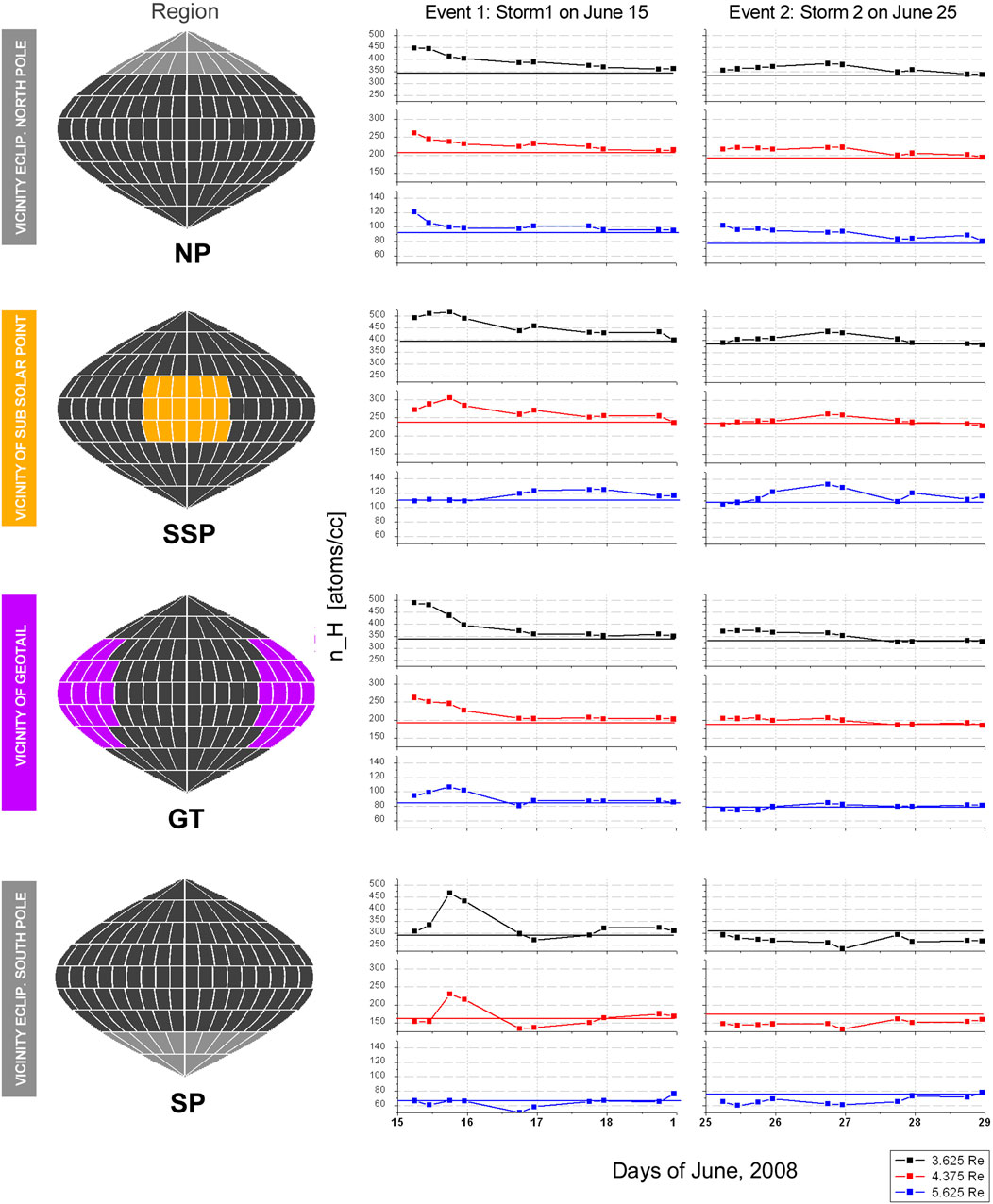
Figure 6. Timelines of regional averaged H densities for both minor storms at distances of 3.6 R_e (black), 4.4 R_e (red), and 5.6 R_e (blue). The values are calculated from the 3-D H-density models shown in Figures 4, 5. The presented regions, marked in different colors on the left column, are the vicinities of the ecliptic North Pole (NP), the sub-solar point (SSP), the geotail (GT), and the ecliptic south pole (SP). The horizontal colored lines within the plots represent the H-density level of the quiet day prior to the storm. For Storm1: Immediately at the beginning, the maximal affected are the NP (at all three distances) and GT (at the lower and mid-distance) regions. Approximately 18 h later, the SSP and SP regions also reach their maximum peak at the lower and mid-distance; also interesting is the ∼2–3 day time-shifted peak at the upper distance in the SSP region. In the SP region, H-density depletions are visible (mainly at the upper distance). For Storm2: H-density enhancements are lower than Storm1. The continuous variation in SWFP between June 26 and 27 (see Figure 2G) is correlated with broad peaks in region NP and SSP at the end of June 26. The GT region is comparable to the same region of Storm1 but with a much lower level of enhancement. H-density depletions are also visible in the SP region.

Figure 7

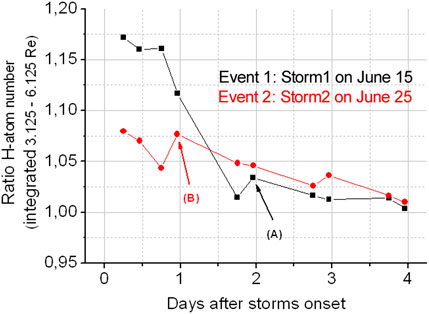
Figure 7. Relative enhancement of the integrated H-atom number between 3 R_e and 6 R_e during Storm1 and 2 with respect to the quiet reference days prior to the two storms. In this radial range, storm 1 (June 15) enhanced the H-atom number at the beginning up to ∼17%, while Storm2 (June 25) enhanced it by ∼8% only. This factor ∼2 stronger impact of storm1 relative to storm2 regarding the neutral H geocorona enhancement lasts for the first ∼1.5 days after onset. From day 2 to the end, the H-density enhancements of both storm recoveries are very similar to their undisturbed values prior to the storms. The marks (A, B) indicate re-enhancement of the H-atom number due to sub-disturbances within the main storms. In the case of Storm2 [see (B)], this was caused by a second incoming flow pressure wave late at night on June 25, which had an amplitude similar to the primary wave in the early morning of June 25.

The total number of exospheric H atoms between 3 R_e and 6 R_e was found to be maximum enhanced by approximately 17.5% for Event1 compared to 8.5% for Event2 (with respect to the H-atom number of a quiet reference day prior to the event). These maximum values and their time dependency during the recovery phase are shown in Figure 7. The effects of the two minor events, Sub1 and Sub2, are also recognizable in our 3-D inversions (i.e., see as marked in Figure 7).

With the beginning of day 2 after onset, the initial difference of the impact levels (by a factor of ∼2) between Event1 and Event2 mostly vanished. In the following days, the exospheric disturbances of both events recover similarly. This can be seen from the ratio of the total H-atom numbers (Figure 7).

3.2.2 Regionally enhanced H densities

Event1 and 2 induce a highly asymmetric H-density enhancement on the dawn with respect to the dusk side. Preferred at lower distances, the higher H-density values were found on the dawn side (see Figures 4, 5, left column) with maximum values near the ecliptic. The level of this asymmetry varies over time, but the dawn-side enhancements persist from the onset to the end of recovery of both events. In Figure 6, the regional averaged H densities for the vicinities of the sub-solar point (SSP), geotail, and the two ecliptic poles are presented for the same three distances as used in Figures 4, 5.

Among the very first affected regions after onset are the geotail (at lower distances) and the North Pole (at upper distances).

Figure 8

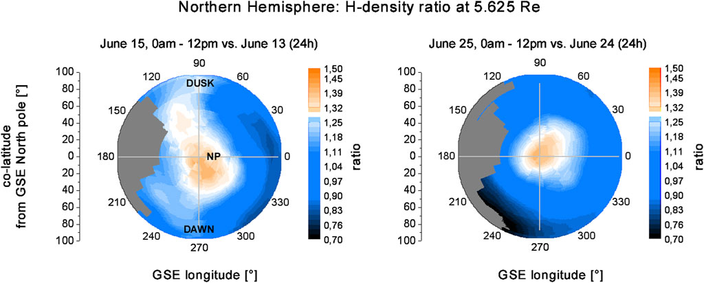
Figure 8. Local relative H-density enhancements in the north polar region at 5.6 R_e observed at the onsets of Storm1 (left) and Storm2 (right). The polar plot images show the top–down view from the North Pole to the northern hemisphere (both in GSE) of the shell at 5.6 R_e. There is a very local H-density enhancement (30%–40%) over the North Pole that starts immediately at storm onset at 5.6 R_e. Other regions at this distance are not or only weakly enhanced in the northern hemisphere at this early storm phase. An exception in the form of an H reduction can be seen for Storm2 (right) near the ecliptic at ∼ 240° GSE longitude. Gray areas represent regions that are not covered by LOS observations with Earth tangent points between 3 and 6 R_e.

Timelines of regionally averaged H densities (separately for the vicinities of the geotail, the sub-solar point, and the two ecliptic poles) are shown in Figure 6 for three distances (3.6 R_e, 4.37 R_e, and 5.6 R_e). They can be summarized as follows:

• In the ecliptic north polar area: Immediately after onset, both storms show a rapid ∼35% H-density enhancement at the upper distance (also shown in Figure 8). For Event1, this peak value lasts for a few hours only. The decline process (recovery) back to the prior H-density values remained for ∼3 days after storms began, which is approximately 1 day longer than in the geotail region.

• At the Earth dayside (in the vicinity of the sub-solar point): Event1 shows a significant peak at the lower and middle distance near the end of the first day, which is followed by a relatively long recovery duration (∼3 days). At these two distances, this region has, in total, the longest period (∼4 days) of enhanced H densities of all regions discussed. Furthermore, for Event1, we found a remarkably time-delayed peak value of the H-atom enhancement at the dayside near the sub-solar point (SSP) at the upper distance. At this location, the H-atom number slowly grows over the first ∼2 days until it reaches its peak value (see also Figures 4, 5, right column). There, the H-atom enhancement remains high for ∼1–1.5 days. At this time, most of the other regions show heavily falling H densities already. A similar effect is also visible for Event2, but with the difference that the density peaks there are shifted at all three distances to the middle of the storm.

• At the Earth nightside (in the vicinity of the geotail): Also immediately after onset, the H-atom enhancement at the lower and mid-distance is recognizable for the first 2 days of both storms. It is stronger for Event1 than Event2. In addition, for both storms, the H-atom number in this region returned during the 2 days relatively quickly to its undisturbed level.

• In the ecliptic South Pole area, only Event1 shows a significant enhancement at the lower and mid-distance between the middle of day 1 and the middle of day 2. At the upper distance—and also for Event2 at all three distances—there is a continuous H-density depletion (instead of an enhancement) visible during both storms. The observational coverage of the ecliptic South Pole area by TWINS LAD is very incomplete compared to the North Pole area. Therefore, it is difficult to determine whether this H-density depletion effect is real or an artifact due to insufficient southern coverage. We acknowledge that a study with better southern coverage is needed to draw firm conclusions in this region.

3.2.3 Correlation with exobase conditions (NRLMSIS)

Our results show that during geomagnetic disturbances, the time dependencies of exobase temperature T_exo and exospheric H-density enhancement (at 3–6 R_e) are very similar and positively correlated. This means that an increase of T_exo at ∼500 km (exobase) is followed by an H-density enhancement in the upper exosphere above 3 R_e. This can be seen in Figure 2, where panel (I) represents the NRLMSIS exobase temperature, and panel (H) shows the Lyman-α column brightness variation as a measure of the varying column H-density above 3 R_e.

Interestingly, the H densities at the exobase (obtained from the NRLMSIS model) respond with a significant reduction to geomagnetic disturbances (see Figure 2J). This anti-correlation of H density and T_exo at the exobase is inverse of what we found for the upper exosphere above 3 R_e. This supports the theory that during a geomagnetic storm, neutral H atoms are transported from the exobase to upper exospheric layers due to the T_exo increase. It will be important to answer the question of how much of those up-flowing H atoms will be lost (due to escape or interaction processes), but that is beyond the scope of this study.

At the storm’s onset, in particular, both polar regions experienced a significantly larger T_exo increase than others. On June 15 (onset of Event1), the T_exo increased by ∼40% at the South Pole and by ∼20% at the North Pole (see Figure 9 – left image). Event2 produced lower T_exo, increases (by 50%) at its onset on June 25 (see Figure 9 – right image).

Figure 9

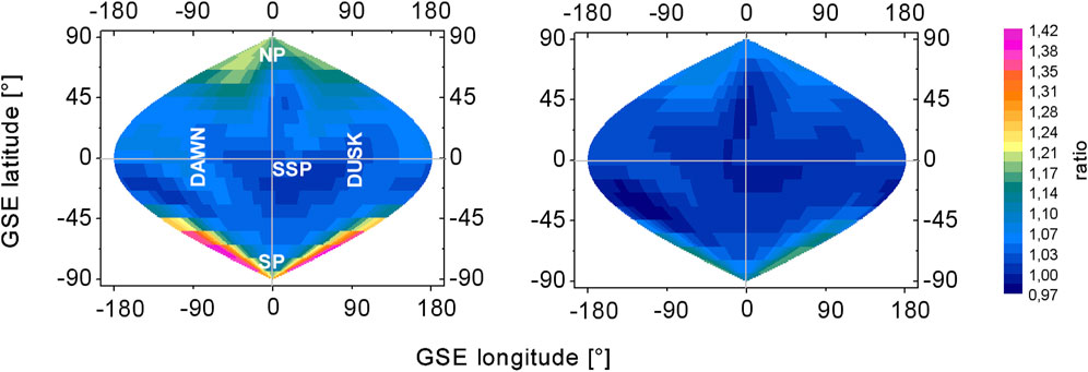
Figure 9. Relative increase of the exobase temperatures T_exo (NRLMSIS) at storm onsets (left: Storm1, June 15, 0–12 p.m.; right: Storm2, June 25, 0–12 p.m.) compared to the temperatures of the quiet reference days prior to the storms. A generally larger T_exo increase caused by Storm1 compared to sStorm2 can be seen. Mostly affected are both polar regions. In particular, there is a significantly larger T_exo increase at the South Pole for Storm1.

In the case of the high T_exo increase at the South Pole on June 15, we found a significant H-atom number enhancement at the southern hemisphere later on this day (see Figure 4 – left and middle column). In addition, in the north polar region, there is an H-density enhancement visible in our 3-D results.

The NRLMSIS empirical model describes the global atmospheric dynamics from the ground to the exobase (Picone et al., 2002; Emmert et al., 2021). In this study, we have used the Python wrapper “pymsis,” which provides immediate access to the NRLMSIS tools. The inputs to run this model under storm-time conditions are the daily F10.7 index, the 81-day average F10.7 centered on the given day, and the Ap index for the last 57 h prior to the given time organized in 3-h average. The general validity of our results must be proven with further investigations of more periods at different solar cycle activity levels.

3.2.4 Error of the 3-D inversions

The upper row of Figure 10 shows the linear relationship between observed and modeled LOS column brightness—exemplary for a quiet day (June 13) and the strongly disturbed time interval at Storm1’s onset (June 15, 0–12 p.m.). Both images present a narrow point distribution, which is very closely located to the ideal zero-error line (gray line). The inversion error is approximately equal for lower and higher column brightness values. This indicates that the quality of the inversion does not vary with distance because column brightness level and LOS Earth tangent point distance are (anti-)-correlated.

Figure 10

Figure 10. Upper row: Point distributions of observed and modeled LOS column brightness exemplary for the quiet day June 13 and the time interval with disturbances at Storm1’s onset (June 15, 0–12 p.m.). The narrow distributions close to the ideal zero-error line (gray line) indicate a small error for both low and high LOS column brightness values, which are associated with the Earth tangent point distance of the LOS. Lower row: Histograms of the relative inversion error (ratio of the observed and modeled LOS column brightness) for the two exemplary intervals. The relative errors of 2.4% (quiet day June 13) and 2.8% (disturbed interval June 15) are derived from Gaussian curve fits of these histograms. The larger relative error of the disturbed interval is explainable with short-time H-density variability during the 12 h of the interval.

The relative inversion error can be quantified as the ratio of the observed to modeled LOS column brightness. The lower row of Figure 10 presents histograms and the derived relative inversion errors (as the width of a Gaussian fit) for the two exemplary time intervals. As expected, the relative error during the quiet interval is, at 2.4%, slightly smaller than 2.8% of the disturbed interval. This is explainable with short-time H-density variability during the disturbed interval.

4 Discussion

The time-dependent 3-D reconstruction of H-density distributions at 3–6 R_e derived from optically thin Ly-α observations demonstrated the dynamic behavior of the terrestrial exosphere with 12 h temporal resolution during minor geomagnetic storms. Variability of the density distributions is theorized to be attributed to several drivers that modify the energy partition of both thermal and non-thermal populations of H atoms in the exosphere (Hodges, 1994). The thermal H atoms originate in the mesosphere lower thermosphere (MLT) region, diffuse upward to the exobase, and obtain their energy through continuous collisions with thermospheric particles such as atomic oxygen. Due to this process, the energy distribution of H atoms is assumed to obey a Maxwellian velocity function, where most of the particles, located near the mean velocity, follow ballistic trajectories beyond the exobase. Those H atoms near the tail of the Maxwellian function have sufficient energy to surpass the gravity force and ultimately escape to interplanetary space, especially for those with radially upward velocities. This mechanism is the dominant escape process for thermal H atoms from Earth and is termed Jeans escape (Jeans, 1923; Chamberlain, 1963; Brinkmann, 1970). On the other hand, non-thermal H atoms do not follow the Maxwellian distribution curve, and it is theorized that atoms obtain their energy through charge exchange interaction with ions from the dense and cold plasmasphere. Evidence of the existence of this hot H population (∼1eV) at altitudes as low as ∼300 km has been reported by Qin and Waldrop (2016) based on the analysis of Ly-$\alpha$ observations acquired by the Global Ultraviolet Imager (GUVI) instrument onboard NASA’s Thermosphere Ionosphere Mesosphere Energetics and Dynamics (TIMED) mission. The study reported that TIMED/GUVI observations during solar minimum conditions could not be fitted to a fully thermal Chamberlain exospheric model but required the inclusion of an additional component with a larger scale height. The authors suggested that the low-altitude hot H atoms may arise through charge exchange interaction with plasmaspheric ions.

The comparison between our results of 3-D hydrogen density distributions and the exobase parameters estimated by the NRLMSIS model (see Figure 2) for the same period indicates the rapid response of the thermal H-atom population to the increased exobase temperatures during the evolution of the geomagnetic storm. The variation of neutral temperature near the exobase occurs initially at the magnetic poles due to particle precipitation in the auroral and cusp regions from the inner magnetospheric ring current and the solar wind, respectively (Zhang et al., 2019; Koike and Taguchi, 2024). These particles, including ions and electrons, interact with neutrals in a process known as Joule heating (Richmond, 2021), which increases the temperature in the polar regions. This polar increase of temperature propagates then to low-latitudes in a few hours. As the lightest element, atomic H rapidly responds to subtle changes in temperature. Increasing temperatures enlarge the population of H atoms on ballistic trajectories with higher apogees as well as the amount of escaping H.

Specifically, we observed variations of temperature of ∼20% at the North Pole, ∼40% at the South Pole, and ∼<10% at the ecliptic plane during the main phase of the June 15 storm with respect to temperature distributions during the quiet-time June 13 (see Figure 9, left panel). With a higher temperature, H atoms increase their velocities, allowing them to reach higher altitudes following ballistic trajectories or even enhancing the escape of particles to space. Although the previous statement may explain the enhancement of H densities at the poles, we also found a significant increase of H-atom density near the dawn and ecliptic plane region that occurs within the June 15 00UT to 12UT period (Figure 4 row 2) at least 6 h before the density enhancement in the Southern hemispheric region. The increase of low-latitude H density is unlikely to be solely associated with variations of the exobase temperature, particularly because low-latitude T_exo does not vary significantly during this period (<∼10%) (see Figure 9). Such an increase in H densities may be associated with the rapid storm-time exosphere-plasmasphere interaction.

Based on continuous observations (90-min cadence) of optically thin H Ly-$\alpha$ emission, Kuwabara et al. (2017) stated that the reduction of the plasmasphere (density and size) during storm time reduces the rate of charge exchange interactions with exospheric H atoms, ultimately resulting in more thermal H particles with a lower energy around the plasmapause (3∼4 R_e). For the sake of clarification, during the quiet time, the plasmasphere typically accelerates a small number of H atoms (due to the small charge exchange cross section), allowing some of them a rapid escape from the plasmaspheric region. During a geomagnetic storm, the increased solar wind pressure induces convection electric fields strong enough to facilitate the outward movement of ions from the plasmasphere toward the high-altitude dayside magnetosphere in the form of structures known as plumes (Darrouzet et al., 2009). This process significantly reduces the plasmaspheric ion population, which results in a movement of the plasmapause closer to Earth. Such a reduction in the plasmaspheric ion population also depletes charge exchange with exospheric H atoms, which in turn reduces the number of H atoms that can reach higher altitudes or even escape. This can be interpreted as a contribution to the increase of the H-density at ∼3–4 R_e. In the analyzed storm period, the plasmapause is located near the ecliptic plane and, using the kp index and the Moldwin et al. (2002) formulation, the plasmapause moved inward from ∼5 R_e to ∼4 R_e during the main phase of the storm. This theory may explain the increase of H density near the ecliptic plane. Notwithstanding, as seen in our results, such an H enhancement occurs mainly in the dawn region. The dusk region, which has the highest exobase temperature around the planet, also has the lowest exobase H density. It suggests that this H depletion at the exobase is somehow maintained at high altitudes. A similar feature has also been observed in previous quiet-time reconstructions reported by Zoennchen et al. (2024).

In addition, our results for the June 15 storm show a delayed H enhancement of the dayside nose (near the sub-solar point) at the highest shell (5.625 R_e), which reaches its maximum density value ∼2 days after the storm onset. Using a non-sophisticated calculation, we found that (5.625–3.625) R_e/2 days = ∼70 m/s is the bulk velocity of the radially upward propagation of atomic H. This value is in excellent agreement with the upwelling velocity found in Cucho-Padin and Waldrop (2019) of ∼60 m/s. Further analysis should be conducted to correlate this velocity value with (1) the specific variations of exobase conditions during the storm, (2) the time dependency on the exosphere-plasmasphere interactions, and (3) the force exerted on H atoms by the permanent solar radiation pressure.

In sum, measurements of H Ly-$\alpha$ emissions acquired by TWINS/LADs and their use to reconstruct 3-D H densities allowed us to analyze the dynamic response of the exosphere to minor geomagnetic storms during solar minimum conditions. Notwithstanding, the lack of spatial coverage and the limited acquisition cadence of our current dataset do not permit a complete understanding of how several drivers may affect the exospheric structure and density. One solution to overcome this problem is the implementation of physics-based models that incorporate the response of the exosphere to exobase conditions and the dynamic plasmaspheric densities, especially during a solar minimum when the number of non-thermal H atoms becomes significant with respect to the total exospheric neutral population (Qin et al., 2017). In the next years, NASA’s Carruthers Geocoronal Observatory mission, to be launched in 2025, will provide an excellent opportunity to observe the terrestrial exosphere with high cadence and sufficient spatial coverage. Our data-analysis methodology is planned to provide support to the science objectives of this mission and primarily investigate the time-dependent response of the exosphere to space weather.

Data availability statement

Publicly available datasets were analyzed in this study. These data can be found here: https://omniweb.gsfc.nasa.gov/.

Author contributions

JZ: writing – original draft and writing – review and editing. GC-P: writing – original draft and writing – review and editing.

Funding

The author(s) declare that financial support was received for the research and/or publication of this article. This research has been supported by the Deutsche Forschungsgemeinschaft (grant no. 469043535) and the NASA Goddard Space Flight Center through Cooperative Agreement 80NSSC21M0180 to Catholic University, Partnership for Heliophysics and Space Environment Research (PHaSER).

Acknowledgments

The authors gratefully thank the TWINS team (PI Dave McComas and PI of the LAD instruments Hans J. Fahr) for making this work possible. Jochen Zoennchen gratefully acknowledges the funding by the Deutsche Forschungsgemeinschaft (DFG, German Research Foundation, grant no. 469043535) and the support of the Argelander Institut für Astronomie at the University of Bonn. We also acknowledge the support from the International Space Science Institute on the ISSI team titled “The Earth’s Exosphere and its Response to Space Weather.” Additionally, we thank the topical editor and the referees for the discussions and the extensive help with improving the article.

Conflict of interest

The authors declare that the research was conducted in the absence of any commercial or financial relationships that could be construed as a potential conflict of interest.

Generative AI statement

The author(s) declare that no Generative AI was used in the creation of this manuscript.

Publisher’s note

All claims expressed in this article are solely those of the authors and do not necessarily represent those of their affiliated organizations, or those of the publisher, the editors and the reviewers. Any product that may be evaluated in this article, or claim that may be made by its manufacturer, is not guaranteed or endorsed by the publisher.

References

Bailey, J., and Gruntman, M. (2011). Experimental study of exospheric hydrogen atom distributions by Lyman-alpha detectors on the TWINS mission. J. Geophys. Res. Space Phys. 116 (19), 1–9. doi:10.1029/2011JA016531

CrossRef Full Text | Google Scholar

Bailey, J., and Gruntman, M. (2013). Observations of exosphere variations during geomagnetic storms. Geophys. Res. Lett. 40, 1907–1911. doi:10.1002/grl.50443

CrossRef Full Text | Google Scholar

Baliukin, I., Bertaux, J.-L., Quemerais, E., Izmodenov, V., and Schmidt, W. (2019). SWAN/SOHO Lyman-α mapping: the hydrogen geocorona extends well beyond the Moon. J. Geophys. Res.-Space 124, 861–885. doi:10.1029/2018JA026136

CrossRef Full Text | Google Scholar

Borovsky, J. E., and Denton, M. H. (2006). Differences between CME-driven storms and CIR-driven storms. J. Geophys. Res. Space Phys. 111, A07S08. doi:10.1029/2005JA011447

CrossRef Full Text | Google Scholar

Brandt, J. C., and Chamberlain, J. W. (1959). Interplanetary gas. I. Hydrogen radiation in the night sky. Astrophysical J. 130, 670–682. doi:10.1086/146756

CrossRef Full Text | Google Scholar

Brinkmann, R. T. (1970). Departures from jeans' escape rate for H and He in the Earth's atmosphere. Planet. Space Sci. 18 (4), 449–478. doi:10.1016/0032-0633(70)90124-8

CrossRef Full Text | Google Scholar

Chamberlain, J. W. (1963). Planetary coronae and atmospheric evaporation. Planet. Space Sci. 11, 901–960. doi:10.1016/0032-0633(63)90122-3

CrossRef Full Text | Google Scholar

Connor, H. K., Jung, J., Qian, L., Sutton, E. K., Cucho-Padin, G., Crow, M., et al. (2024). Storm-time variability of terrestrial hydrogen exosphere: kinetic simulation results. Front. Astronomy Space Sci. 11, 1421196. doi:10.3389/fspas.2024.1421196

CrossRef Full Text | Google Scholar

Cucho-Padin, G., Ferradas, C., Fok, M., Waldrop, L., Zoennchen, J. H., and Kang, S. (2025). The role of the dynamic terrestrial exosphere in the storm-time ring current decay. Front. Astronomy Space Sci. 12, 1533126. doi:10.3389/fspas.2025.1533126

CrossRef Full Text | Google Scholar

Cucho-Padin, G., Kameda, S., and Sibeck, D. G. (2022). The Earth’s outer exospheric density distributions derived from PROCYON/LAICA UV observations. J. Geophys. Res. Space Phys. 127, e2021JA030211. doi:10.1029/2021JA030211

CrossRef Full Text | Google Scholar

Cucho-Padin, G., and Waldrop, L. (2019). Time-dependent response of the terrestrial exosphere to a geomagnetic storm. Geophys. Res. Lett. 46, 11661–11670. doi:10.1029/2019GL084327

CrossRef Full Text | Google Scholar

Darrouzet, F., Gallagher, D. L., André, N., Carpenter, D. L., Dandouras, I., Décréau, P. M. E., et al. (2009). Plasmaspheric density structures and dynamics: properties observed by the CLUSTER and IMAGE missions. Space Sci. Rev. 145, 55–106. doi:10.1007/s11214-008-9438-9

CrossRef Full Text | Google Scholar

Emerich, C., Lemaire, P., Vial, J.-C., Curdt, W., Schühle, U., and Wilhelm, K. (2005). A new relation between the central spectral solar HI Lyman-α irradiance and the line irradiance measured by SUMER/SOHO during the cycle 23. Icarus 178, 429–433. doi:10.1016/j.icarus.2005.05.002

CrossRef Full Text | Google Scholar

Emmert, J. T., Drob, D. P., Picone, J. M., Siskind, D. E., Jones, M., Mlynczak, M. G., et al. (2021). NRLMSIS 2.0: a whole-atmosphere empirical model of temperature and neutral species densities. Earth Space Sci. 8, e2020EA001321. doi:10.1029/2020EA001321

CrossRef Full Text | Google Scholar

Fahr, H. J. (1971). The interplanetary hydrogen cone and its solar cycle variations. Astron. Astrophys. 14, 263–274. Available online at: https://scholar.google.com/scholar?hl=en&as_sdt=0%2C5&q=The+interplanetary+hydrogen+cone+and+its+solar+cycle+variations&btnG=

Google Scholar

Hodges, R. R. (1994). Monte Carlo simulation of the terrestrial hydrogen exosphere. J. Geophys. Res. Space Phys. 99, 23229–23247. doi:10.1029/94JA02183

CrossRef Full Text | Google Scholar

Ilie, R., Skoug, R. M., Funsten, H. O., Liemohn, M. W., Bailey, J. J., and Gruntman, M. (2013). The impact of geocoronal density on ring current development. J. Atmos. Solar-Terrestrial Phys. 99, 92–103. doi:10.1016/j.jastp.2012.03.010

CrossRef Full Text | Google Scholar

Jeans, J. (1923). “The dynamical theory of gases,” in Cambridge library collection - physical sciences (Cambridge University Press), 4. doi:10.1017/CBO9780511694370

CrossRef Full Text | Google Scholar

Khazanov, G. V., Liemohn, M. W., Newman, T. S., Fok, M.-C., and Ridley, A. J. (2004). Magnetospheric convection electric field dynamics andstormtime particle energization: case study of the magneticstorm of 4 May 1998. Ann. Geophys. 22, 497–510. doi:10.5194/angeo-22-497-2004

CrossRef Full Text | Google Scholar

Koike, H., and Taguchi, S. (2024). Ion precipitation in the cusp for northward IMF and its relationship with magnetosheath flow. Earth Planets Space 76, 80. doi:10.1186/s40623-024-02011-w

CrossRef Full Text | Google Scholar

Krall, J., Glocer, A., Fok, M.-C., Nossal, S. M., and Huba, J. D. (2018). The unknown hydrogen exosphere: space weather implications. Space weather. 16, 205–215. doi:10.1002/2017SW001780

CrossRef Full Text | Google Scholar

Kuwabara, M., Yoshioka, K., Murakami, G., Tsuchiya, F., Kimura, T., Yamazaki, A., et al. (2017). The geocoronal responses to the geomagnetic disturbances. J. Geophys. Res. Space Phys. 122, 1269–1276. doi:10.1002/2016JA023247

CrossRef Full Text | Google Scholar

Lin, M.-Y., Cucho-Padin, G., Oliveira, P., Glocer, A., and Rojas, E. (2024). Variability of Earth’s ionospheric outflow in response to the dynamic terrestrial exosphere. Front. Astron. Space Sci. 11, 1462957. doi:10.3389/fspas.2024.1462957

CrossRef Full Text | Google Scholar

McComas, D. J., Allegrini, F., Baldonado, J., Blake, B., Brandt, P. C., Burch, J., et al. (2009). The two wide-angle imaging neutral-atom Spectrometers (TWINS) NASA mission-of-opportunity. Space Sci. Rev. 142 (1–4), 157–231. doi:10.1007/s11214-008-9467-4

CrossRef Full Text | Google Scholar

Moldwin, M. B., Downward, L., Rassoul, H. K., Amin, R., and Anderson, R. R. (2002). A new model of the location of the plasmapause: CRRES results. J. Geophys. Res. Space Phys. 107 (A11), 2–9. doi:10.1029/2001JA009211

CrossRef Full Text | Google Scholar

Nass, H. U., Zoennchen, J. H., Lay, G., and Fahr, H. J. (2006). The TWINS-LAD mission: observations of terrestrial Lyman-α fluxes. ASTRA Astrophysics Space Sci. Trans. 2, 27–31. doi:10.5194/astra-2-27-2006

CrossRef Full Text | Google Scholar

Nilam, B., Ram, S. T., Shiokawa, K., Balan, N., and Zhang, Q. (2020). The solar wind density control on the prompt penetration electric field and equatorial electrojet. J. Geophys. Res. Space Phys. 125, e2020JA027869. doi:10.1029/2020JA027869

CrossRef Full Text | Google Scholar

Østgaard, N., Mende, S. B., Frey, H. U., Gladstone, G. R., and Lauche, H. (2003). Neutral hydrogen density profiles derived from geocoronal imaging. J. Geophys. Res. Space Phys. 108 (A7), 1–12. doi:10.1029/2002JA009749

CrossRef Full Text | Google Scholar

Picone, J. M., Hedin, A. E., Drob, D. P., and Aikin, A. C. (2002). NRLMSISE-00 empirical model of the atmosphere: statistical comparisons and scientific issues. J. Geophys. Res. Space Phys. 107 (A12), 15–16. doi:10.1029/2002JA009430

CrossRef Full Text | Google Scholar

Qin, J., and Waldrop, L. (2016). Non-thermal hydrogen atoms in the terrestrial upper thermosphere. Nat. Commun. 7, 13655. doi:10.1038/ncomms13655

PubMed Abstract | CrossRef Full Text | Google Scholar

Qin, J., Waldrop, L., and Makela, J. J. (2017). Redistribution of H atoms in the upper atmosphere during geomagnetic storms. J. Geophys. Res. Space Phys. 122 (10), 10,686–10,693. doi:10.1002/2017JA024489

CrossRef Full Text | Google Scholar

Richmond, A. D. (2021). “Joule heating in the thermosphere,” in Upper atmosphere dynamics and Energetics. Editors W. Wang, Y. Zhang, and L. J. Paxton doi:10.1002/9781119815631.ch1

CrossRef Full Text | Google Scholar

Snow, M., Reberac, A., Quémerais, E., Clarke, J., McClintock, W. E., and Woods, T. N. (2013). “A new catalog of ultraviolet stellar spectra for calibration,” in Cross-calibration of far UV spectra of solar system objects and the heliosphere (New York: Springer Science and Business Media), 13, 191–226. doi:10.1007/978-1-4614-6384-9_7

CrossRef Full Text | Google Scholar

Thomas, G. E. (1978). The interstellar wind and its influence on the interplanetary environment. Annu. Rev. earth Planet. Sci. 6 (1), 173–204. doi:10.1146/annurev.ea.06.050178.001133

CrossRef Full Text | Google Scholar

Zhang, Y., Paxton, L. J., Lu, G., and Yee, S. (2019). Impact of nitric oxide, solar EUV and particle precipitation on thermospheric density decrease. J. Atmos. Solar-Terrestrial Phys. 182, 147–154. doi:10.1016/j.jastp.2018.11.016

CrossRef Full Text | Google Scholar

Zoennchen, J. H., Cucho-Padin, G., Waldrop, L., and Fahr, H. J. (2024). Comparison of terrestrial exospheric hydrogen 3D distributions at solar minimum and maximum using TWINS Lyman-α observations. Front. Astron. Space Sci. 11, 1409744. doi:10.3389/fspas.2024.1409744

CrossRef Full Text | Google Scholar

Zoennchen, J. H., Nass, U., and Fahr, H. J. (2015). Terrestrial exospheric hydrogen density distributions under solar minimum and solar maximum conditions observed by the TWINS stereo mission. Ann. Geophys. 33, 413–426. doi:10.5194/angeo-33-413-2015

CrossRef Full Text | Google Scholar

Zoennchen, J. H., Nass, U., Fahr, H. J., and Goldstein, J. (2017). The response of the H geocorona between 3 and 8 R_e to geomagnetic disturbances studied using TWINS stereo Lyman-α data. Ann. Geophys. 35 (1), 171–179. doi:10.5194/angeo-35-171-2017

CrossRef Full Text | Google Scholar