Simultaneous observations of irregular sporadic E structures using the LWA and a DPS4D

Multi-instrument studies have recently shed new light on the morphology of sporadic E, especially intense sporadic E. Here we present simultaneous observations of dense sporadic E (${\text{E}}_s$) structures using the Long Wavelength Array (LWA) radio telescopes and a Digisonde Portable Sounder 4D (DPS4D). Our coordinated observations show that the LWA radio telescopes in central New Mexico can reliably locate regions of dense Es structures as they pass over a Digisonde located over 500 km away in Texas. The LWA appears to be most sensitive to the densest E_s structures, which also appear to contain irregularities with vertical structure, possibly indicating turbulence. These irregularities cause off-zenith backscatter, as observed by the DPS4D, and are observed to move at speeds of a few tens of m/s. The irregularities also appear to act as a phase screen, producing short-lived daytime spread F and E conditions. We hypothesize that turbulent structures driven by the Kelvin–Helmholtz (KH) instability may be responsible for the observations.

1 Introduction

In recent years, numerous studies have shed new light on the morphology of sporadic E (${\text{E}}_s$). Of particular interest is the morphology associated with severe events, where the peak frequency of the ${\text{E}}_s$ (${\text{foE}}_s$) greatly exceeds the typical values. Using Global Navigation Satellite System (GNSS) total electron content (TEC) tomography over Japan, Maeda and Heki (2014) and Maeda and Heki (2015) showed that high-density ${\text{E}}_s$ events are often oriented in discrete, front-like structures spanning hundreds of km in length but only a few km in width. Sun et al. (2018) made similar observations of front-like structures over China using the Beidou Ionospheric Observation Network (BION) (Hu et al., 2017). Obenberger et al. (2021) showed that discrete clouds of high-density ${\text{E}}_s$ could be imaged and tracked with the Long Wavelength Array (LWA) radio telescopes. The clouds were often arranged in propagating fronts similar to the previous measurements using GNSS. These observations show fronts forming during both day and nighttime conditions with no obvious difference between the two.

The GNSS-observed structures may be related to the quasi-periodic (QP) echoes observed by very high frequency (VHF) coherent scatter radars (Yamamoto et al., 1994; Chu and Wang, 1997; Hysell and Burcham, 2000; Saito et al., 2006). QP echoes, however, are primarily observed at nighttime, when elongated fronts of field-aligned irregularities (FAIs) can exist, and they are typically observed to propagate to the southwest (in the Northern Hemisphere). The nighttime coupling between the E and F layers is also believed to produce the observed mid-latitude spread F, which is often coincident with VHF observations of QP echoes (Tsunoda and Cosgrove, 2001; Haldoupis et al., 2003). QP echoes are observed to have spatial scale sizes similar to the fronts measured by GNSS tomography and the LWA. However, the fronts observed by Maeda and Heki (2014) and others are a common feature of both daytime and nighttime E_s. Moreover, they are observed to move in many directions—not just southwestward. Although it is possible that these two types of front-like ${\text{E}}_s$ structures are completely different phenomena, it is also possible that irregularities that trigger QP echoes are a subset of the more general type (Maeda and Heki, 2014).

Sun et al. (2020) combined GNSS tomography with two ionosondes and two VHF radars to observe a case of strong daytime Es, during which two front-like events passed over southern China. As shown by the GNSS tomography, the front-like events move over the region, and both the ionosondes and the radars observed an approaching and then departing structure in range. This movement manifested in the range–time–intensity (RTI) plots from the VHF radars as a “V” shape. For the ionosondes, the approaching structure had a peak frequency of at least 17 MHz, indicating an exceptional event. The results clearly showed that the front-like structure was associated with irregular three dimensional (3D) structure, capable of creating backscatter at both HF and VHF frequencies over a range of angles. Patra et al. (2012) reported a similarly shaped range-time structure, as observed from the Gadanki radar at 53 MHz. The described “U”-shaped structure was coincident with a strong ${\text{E}}_s$ layer, observed to have an ${\text{foE}}_s$ of 16 MHz. We note that Sun et al. (2020) described the structures as “V”-shaped, which the authors of this study believe to be a slightly more accurate description than the “U” shape used by Patra et al. (2012).

Larsen (2000) proposed that the same wind shear that forms ${\text{E}}_s$ could also produce Kelvin–Helmholtz (KH) billows in the neutral thermosphere and could, therefore, provide the free energy to drive the larger-scale FAIs of QP echoes. A model presented in Bernhardt (2002) shows that the KH instability would produce billows of dense plasma with separation on the order of a few kilometers to a few tens of kilometers. High-resolution Ca⁺ lidar measurements presented by Ejiri et al. (2019) show clear vertical structures in ${\text{E}}_s$, likely caused by KH instabilities. Similarly, fine structures observed using the Arecibo incoherent scatter radar may have also been caused by KH instabilities (Hysell et al., 2009; Hysell et al., 2012). Hysell and Larsen (2021) and Bui et al. (2023) provided further evidence that QP echoes are driven by KH instability and, more generally, by Ekman-type instability, which arises from turning shears. Both Patra et al. (2012) and Sun et al. (2020) interpreted their daytime VHF backscatter results as likely being caused by a turbulent ${\text{E}}_s$ layer, which could have been driven by KH or Ekman instabilities.

Much of the aforementioned modeling work on ${\text{E}}_s$ instabilities was undertaken in the context of explaining QP echoes. KH and Ekman instabilities, however, do not themselves generate the FAIs responsible for QP echoes. Instead, they would initiate the formation of FAIs during nighttime conditions through a different process. During the day, large FAIs and spread F may not form as readily due to strong photoionization from the Sun and the presence of the F1 layer, which shorts out the E field between the E and F2 layers. Smaller-scale non-field-aligned plasma irregularities, however, are still expected to be present in the E layer due to KH and Ekman instabilities.

The technique described by Obenberger et al. (2021) allows us to track intense ${\text{E}}_s$ structures using the LWA radio telescopes. As described in that study, the LWA radio telescopes observe ${\text{E}}_s$ as discrete clouds of emission, often arranged in a front-like formation. Obenberger et al. (2021) presented strong evidence that much of the observed emission was the result of forward scatter of broadband noise. The brightest events occurred when the ${\text{E}}_s$ was at the mid-point between an LWA and a large population center where most of the anthropogenic noise is created. This passive technique allows for tracking of ${\text{E}}_s$ over a wide area. It is not known, however, whether all of the emission results from forward scatter or other scattering mechanisms. Self-generated emission also remains a possibility.

In this paper, we present a Digisonde Portable Sounder 4D (DPS4D) and passive LWA radio telescope observations captured over a six-month period centered on the summer of 2022. We examine strong ${\text{E}}_s$ events, which display many characteristics similar to those observed by Sun et al. (2020) and Patra et al. (2012). Furthermore, we examine five cases where high-quality LWA image data clearly show ${\text{E}}_s$ structures moving over the region of the DPS4D. This experiment shows that the LWA is an effective tool for tracking strong ${\text{E}}_s$ events and provides evidence that cases of strong ${\text{E}}_s$ are caused by discrete moving regions of turbulent plasma. The remainder of this paper is organized as follows: Section 2 provides a description of the experiment, Section 3 describes the results, Section 4 discusses the results in the context of past ${\text{E}}_s$ observations, and Section 5 presents our conclusions.

2 Description of the experiment

The observations for this experiment were carried out during the summer of 2022. The experiment itself was largely a follow-on study to Obenberger et al. (2021), which showed that ${\text{E}}_s$ tracking was possible but did not carry out a study demonstrating the utility of the new capability. To test the LWA’s accuracy in locating and characterizing E_s, we deployed a dedicated DPS4D in the field of view of the LWA radio telescopes. Moreover, we use the opportunity to better understand how ${\text{E}}_s$ manifests in ionosonde measurements by taking into account the ${\text{E}}_s$ location and morphology provided by the LWA.

2.1 DPS4D observations/analysis

For this study, we deployed a DPS4D (see Reinisch et al. (2008) and Reinisch et al. (2009) for more details on the DPS4D) to a Pecos County property in Ft. Stockton, TX (30.888 N; 102.832 W). We operated the DPS4D to produce one ionogram every 5 minutes (288 ionograms per day) at frequencies between 2 and 20 MHz, using both ordinary mode (O-mode) and extraordinary mode (X-mode) polarizations. We operated the DPS4D receive array in the standard equilateral triangle configuration, but, due to space constraints, we reduced the size of the triangle from 60 m on a side to 30 m, as suggested by the DPS4D manual (https://digisonde.com/pdf/Digisonde4DManual_LDI-web.pdf). This configuration preserved our ability to distinguish off-zenith reflections and acquire estimates of the azimuthal directions of returns.

Aside from a few short periods of power outages, the DPS4D in Ft. Stockton operated continuously from 13 April 2022 until 17 October 2022. Both the processed Portable Network Graphics (PNG) and Routine Scientific Format (RSF) files were archived for the entire data collection window, totaling approximately 80 GB of data. The RSF files, which contain the raw ionograms (power as a function of range and frequency) and the angle of arrival information, were used for the analysis presented in this paper. The PNG files, which show the plotted ionograms and the angle of arrival information, were useful primarily for quick looks at the data.

The RSF ionograms were processed to remove radio frequency interference (RFI). This was carried out using a simple spectral subtraction technique. Since RFI is generally a narrow band feature and occurs at all ranges equally, we simply subtracted the median spectra from each ionogram. The median was used because it largely ignores the radar returns, which are generally limited to a few range bins per frequency. The left panel of Figure 1 shows a raw O-mode ionogram before the background is removed, and the center panel shows the same ionogram after removal.

Figure 1

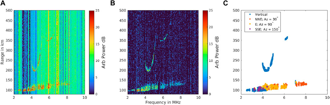
Figure 1. Ionogram produced by the Ft. Stockton DPS4D on 18 June 2022. (A) Raw ionogram, (B) ionogram with median spectrum removed, and (C) identified returns from the ionogram, with colors indicating their azimuthal direction.

Once the noise is reduced, we can search for ${\text{E}}_s$ by simply finding pixels above a particular threshold. Since we are looking for large connected structures, we can further isolate returns by only using bright pixels that are connected to at least 10 other bright pixels. For automatically identifying Es, we use a range between 90 and 150 km. The highest frequency matching these parameters is identified as the peak plasma frequency of the ${\text{E}}_s$ (${\text{foE}}_s$). For the ionogram shown in Figure 1, we found an ${\text{foE}}_s$ of 8.1 MHz using a threshold of 6 dB.

Additionally, the right panel in Figure 1 shows the estimated angle of arrivals from the returns. The DPS4D records the angle of arrival by beamforming in seven directions, and the direction of a given return is determined by the beam in which it appears the brightest. The first beam is vertical (at zenith), and the other six are at zenith angles of 30$°$ and separated by 60$°$ in azimuth. Measuring azimuth from north $(0°)$, with the value increasing eastward, the six oblique beams were at azimuths of 30$°$, 90$°$, 150$°$, 210$°$, 270$°$, and 330$°$. The ionogram shown in Figure 1 displays vertical returns from both the E and F layers and off-zenith returns—up to $\sim$ 8 MHz—from spread ${\text{E}}_s$ to the north–northeast (NNE) and east (E).

2.2 LWA observations/analysis

At the time of the experiment, two LWA stations were operational in central New Mexico. The first station, LWA1, is co-located with the Very Large Array at 34.0689 N, 107.6283 W (Ellingson et al., 2013). The second station, LWA-SV is located at Sevilleta National Wildlife Refuge with a latitude and longitude of 34.3484 N and 106.8858 W, respectively (Cranmer et al., 2017). LWA-SV is approximately 75 km northeast of LWA1 and 540 km northwest of Ft. Stockton. Each station consists of 256 dual-polarization bent dipole antennas pseudo-randomly spaced over a 100 × 110 m ellipse with one or more additional outrigger antennas for calibration.

Both LWA stations are capable of beamforming and all-sky imaging. For this paper, we utilized the all-sky imaging capabilities, where the raw voltages from each antenna are cross-correlated and imaged to produce all-sky maps. For more details on LWA all-sky imaging, see Obenberger et al. (2015). The LWA all-sky imager (LASI) at LWA1 uses 100 kHz of bandwidth and can be tuned anywhere in the 10–88 MHz usable frequency range. Typically, LASI is tuned to 38.1 MHz, and all of the LWA observations used in this paper were at 38.1 MHz. LWA-SV has an upgraded version of LASI, called Orville, which uses a new graphical processing unit (GPU)-based correlator (Varghese et al., 2021). This new imager is capable of capturing 19.8 MHz of bandwidth, which is initially channelized into 198 bins (100 kHz each). The full-resolution images are kept for 2 weeks, but frequency-averaged images with six bins are stored indefinitely. During this experiment, the imager was centered at 30 MHz and imaged from approximately 20 to 40 MHz. Both stations produce 5-second averaged snapshots, resulting in 720 images per hour.

As demonstrated by Obenberger et al. (2021), both LWA stations can image and geolocate discrete clouds of Es. Obenberger et al. (2021) showed that at least some of the observed emissions come from unintentional anthropogenic noise, likely originating from power lines and other sources of broadband radio emissions. However, we note that it is currently unclear whether this accounts for all of the observed emissions. Assuming that the altitude of the ${\text{E}}_s$ is near 100 km, the location of the cloud can be estimated from a single station provided that the zenith angle is less than $\sim$ 20°. At greater zenith angles (low elevation angles), the Cartesian projection of the image prevents precision zenith angle estimates, and the position error increases. However, because both stations can observe discrete ${\text{E}}_s$ clouds, their location can be better geolocated using simple tomography techniques.

The intention of this experiment was to operate both LWA stations throughout the entire period of time during which the DPS4D was deployed to Ft. Stockton. However, due to maintenance issues at both stations, continuous co-observations did not occur. LWA-SV began experiencing cooling issues in early July and missed the majority of July. Similarly, LWA1 experienced computer hardware failures in mid-July and missed the second half of the month through the end of August. Therefore, most of the LWA observations presented in this paper occurred in May and June, with a few exceptions. We also note that the LWA was not observing the emissions from the DPS4D. The DPS4D is only transmitting up to 20 MHz, just below the lowest frequencies observed by the LWA. The LWA observations are 100% passive, utilizing broadband anthropogenic noise that scatters off intense ${\text{E}}_s$ clouds.

Before an all-sky image from either station can be used to detect sporadic E, the background sky needs to be removed. To achieve this, we produce a library of all-sky images at every local sidereal time (LST). This library is created by stacking nearly 100 images for a given 5 s LST window, each image from a different day. We then take the median across all the images at a given LST to produce a “model” of the background sky. We use the median because it largely ignores outliers caused by intermittent solar bursts, lightning, and other sources of RFI. After building the LST library, we then used it to remove the background sky from any given image.

Figure 2 shows an example of LWA-SV all-sky image from 18 May 2022 at 1800 UT, captured at 34.9 MHz. It also shows the median background image at the same LST and the result of subtracting the median image from the image obtained on 18 May. As can be seen, the constant galactic emission is removed, leaving only the transient phenomenon. The excess emission to the south and southeast is from Es, but the emission to the north is from local RFI, namely, a noisy inverter on a nearby recreational vehicle parked at the Sevilleta National Wildlife Refuge. Other features, such as the sun (just southeast of the zenith) and scintillating point sources, were removed by zeroing the pixels within 3$°$ of their respective celestial coordinates.

Figure 2

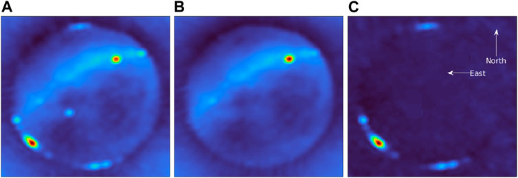
Figure 2. (A) LWA-SV all-sky image captured on 18 May 2022 at 1800 UT, centered at 34.9 MHz. (B) Median background all-sky image for the same LST (02:38 LST) and frequency, similar to the image on the left. (C) LWA-SV image after subtraction of the median background model.

After the background sky is removed, the search for ${\text{E}}_s$ is then carried out. This search is predicated on the idea that the emission from an ${\text{E}}_s$ structure is spatially and temporally constant over a 5-min window but changes (primarily spatially) over 1 h. By subtracting the hourly median from each image, we can mitigate slowly varying, stationary transients such as local RFI. Similarly, by reducing the data to 5 min median data chunks, we can mitigate rapidly varying sources of noise such as lightning. Any remaining bright emissions are likely Es, although we note that some sources of noise remain. Any pixels above a 10-sigma threshold are preserved as potential Es, and any pixels below 10 sigma are masked with zeros (“sigma” refers to the 2D standard deviation of the image).

The final step in the ${\text{E}}_s$ identification process is to combine the masked all-sky images from both stations and grid them onto geographic coordinates. Assuming that the ${\text{E}}_s$ is at an altitude of 100 km, we generated a look-up table for each LWA station that converts the azimuth and elevation of each pixel to geodetic latitude and longitude grid. For each 5 min window, the resulting pixel grids from each station are multiplied together. When both stations agree that an ${\text{E}}_s$ emission is present within the same grid cell, it is mapped at the corresponding latitude and longitude. However, if one station detects emissions in a cell but the other does not, we assume is that there is no ${\text{E}}_s$ there and assign a value of 0. With two stations, this anti-coincidence method removes much of the remaining sources of local interference. The addition of future stations would greatly improve this approach as all stations need to agree that the emission is present for it to be identified as E_s.

Figure 3 shows an example of ${\text{E}}_s$ observations by both stations and the product of the geolocating pipeline. The images from each station also show several local RFI sources that did not make it through the automated pipeline. Each of these sources was constant throughout the hour of data and, therefore, was mostly removed. Notably, ${\text{E}}_s$ is detected at slightly different azimuths from both stations, which allows for geolocation. This particular ${\text{E}}_s$ structure moved to the west during this observation.

Figure 3

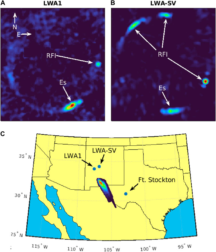
Figure 3. (A) Background-subtracted all-sky image from LWA1 on 6 June 2022 at 1300 UT, showing ${\text{E}}_s$ to the south and local RFI to the east. (B) Background-subtracted all-sky image from LWA-SV from the same time showing the same ${\text{E}}_s$ to the south and three different local RFI sources. (C) Map generated by the ${\text{E}}_s$ geolocating pipeline. Several components can be observed 300 km south of both stations. Note: the east and west directions were reversed from the standard LWA images in order to match the standard geographic map directions.

Parallax observations from two or more stations greatly reduce the positioning error, especially when ${\text{E}}_s$ is low on the horizon, where an accurate zenith angle is difficult—if not impossible—to determine. For instance, the ${\text{E}}_s$ event shown in Figure 3 is observed over the border region of New Mexico. However, from a single station, the probability map would extend well into Mexico and Texas. We note that the result does not become less accurate; it only becomes less precise, covering a much larger impacted region than what parallax observations would indicate. Despite this deficiency, even a single station can be useful and is very precise when ${\text{E}}_s$ is high above the horizon, where zenith angles are easier to measure. Single-station positioning relies on the assumption that intense ${\text{E}}_s$ occurs at an altitude of 100 km, which is likely accurate to within $\pm$ 5 km. Since both stations did not run 100% of the time during the experiment, not all ${\text{E}}_s$ cases presented in this paper contain data from both stations. In particular, LWA1 cannot operate the all-sky mode while other observations (such as beamforming) are taking place. We, therefore, only require that LWA-SV was operational for our analysis. When LWA1 is running, the resolution improves, but LWA-SV data by themselves are still useful for comparison with the DPS4D.

2.3 HF receiver

In addition to the DPS4D at Fort Stockton, we also operated a wide-band HF receiver at LWA-SV. This receiver utilizes a software-defined radio, a magnetic loop antenna, and a large storage RAID system to record signals in the 2–22 MHz range. As described by Obenberger et al. (2023), the receiver is comprised of a magnetic loop antenna, an Ettus ×300 Universal Software Radio Peripheral (USRP), a GPS-synced clock, a PC, and 160 TB RAID. The receiver was configured to listen to the Fort Stockton DPS4D and produce oblique ionograms. Due to the overheating issues at LWA-SV, the receiver was only operated during the first part of the experiment, being shut down on June 06.

The goal of the receiver was to measure the impacts of ${\text{E}}_s$ on oblique propagation in the F layer. At 540-km ground range from Ft. Stockton, the Sevilleta HF receiver was well-suited to measure the effects of sporadic E on the F layer propagation. This distance, however, is too great to simultaneously measure significant changes in propagation from the sporadic E layers, which themselves have only a 20 MHz bandwidth as many of these impacts are expected to be well above 22 MHz.

3 Results

In this section, we describe the results of the experiment. The primary objective of the experiment was to quantify the LWA’s ability to identify and characterize Es. However, we have also found that LWA observations have enabled a better understanding of the common features detected in the ionosonde observations of Es.

3.1 Accuracy of LWA E_s tracking

In this section, we test the accuracy of the LWA radio telescopes to observe ${\text{E}}_s$ conditions above the Fort Stockton DPS4D. An ${\text{E}}_s$ layer at 100 km altitude above the DPS4D would appear at a zenith angle of 82.2$°$ (7.8$°$ elevation angle) from LWA-SV. At such oblique angles, the maximum observed frequency (MOF) for a reflected signal is much higher than the foE_s. We can use the well-known secant law to relate MOF to foE_s as follows:

$MOF=foEs\times \sec \theta ,(1)$

where $\theta$ is incident angle of the ray on the layer. For a perfectly horizontal layer, the incident angle is approximately the same as the zenith angle to that layer. However, we can use the more accurate spherical ionosphere approximation. At a ground range of 540 km and an ionospheric height of 100 km, the incidence angle for a sporadic E layer above Ft. Stockton, observed from LWA-SV, would be 77.3$°$. Using Equation 1, $\sec \theta$ from LWA-SV for a ${\text{E}}_s$ layer at 100 km above the DPS4D is equal to 4.6. For an ${\text{E}}_s$ layer above the DPS4D to appear at LWA-SV at 38 MHz, it would need a minimum ${\text{foE}}_s$ of 8.3 MHz. Similarly, for the layer to be observed from LWA1 at an incidence angle of 77.75$°$, it would require a minimum ${\text{foE}}_s$ of 8.1 MHz. We should note that any tilts caused by tides, gravity waves, and turbulence would alter the incidence angle of the sporadic E layer. This is likely to vary by up to a few degrees depending on the severity of the variations.

To determine the accuracy of the LWA for identifying sporadic E, we compare the instances where LWA-SV did and did not observe emission toward Ft. Stockton to DPS4D measurements of Es. We can use the method described in Section 2.1 to find instances of ${\text{E}}_s$ and estimate foE_s. We can also use the ${\text{E}}_s$-finding algorithm described in Section 2.2 to determine the instances where LWA-SV finds emissions coming from $\pm 5°$ of the E layer above the DPS4D. The value of 5° was chosen because it is roughly the full width at half maximum (FWHM) beam size, or resolution, of the LWA at 38.1 MHz. We can then compare the rate of detection of both systems.

Since we are trying to determine the LWA’s ability to accurately measure ${\text{E}}_s$ over a DPS4D, we use the 5 min DPS4D measurements as “truth.” A plot showing foE/${\text{foE}}_s$ for each day of observation at the Fort Stockton DPS4D is shown in the left panel of Figure 4. As can be seen, a wide range of foE/${\text{foE}}_s$ values were observed, with the maximum being 16 MHz. Here, we do not distinguish between foE and foEs; we simply allow the algorithm explained in Section 2.1 to find any signal in the E region and calculate the maximum frequency. In this particular example, we used an SNR threshold of 12 dB and a minimum number of connected pixels of 10. The background E region can be clearly observed, which typically lasts 1300–0200 UT (0800–2100 LT) near the peak of summer (roughly day 80 of the observations). Typical foE values are approximately 2–3 MHz; however, as can be observed around the local noon, there is a noticeable gap in data where D layer absorption is high and reduces the SNR of the normal E layer below the 12 dB limit.

Figure 4

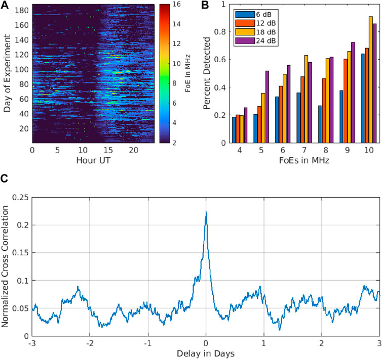
Figure 4. (A) foE measured for each hour of each day of the experiment window. (B) Percent of measured ${\text{E}}_s$ layers that were detected by LWA-SV. ${\text{E}}_s$ “truth” data were provided by the DPS4D and are binned into 1 MHz windows. A separate plot is shown for each threshold level of the ${\text{E}}_s$ detection algorithm. (C) Normalized cross correlation between all DPS4D “truth” data (${\text{E}}_s$ above 5 MHz) and ${\text{E}}_s$ layers detected by LWA-SV.

Using a simple binary system, we assign a value of 1 when the DPS4D measurement detects ${\text{E}}_s$ and LWA-SV detects emissions within $\pm 5°$. Conversely, we assign a 0 when the DPS4D detects ${\text{E}}_s$, but LWA-SV does not detect emission. By summing all the binary data points and dividing the result by the total number of positive DPS4D detections, we can determine the percentage of accuracy of LWA-SV for detecting ${\text{E}}_s$ at the DPS4D. We can also calculate the false positive rate by assigning 1 to events where the DPS4D does not detect ${\text{E}}_s$, but LWA-SV detects emissions in the direction of Fort Stockton. This sum is then divided by the total number of DPS4D non-detections of E_s.

Although we assume that the DPS4D is “truth,” we must keep in mind that ${\text{E}}_s$ is not as simple as a binary (present or not present). Instead, we must run our DPS4D detection pipeline through multiple signal-to-noise ratio (SNR) and ${\text{foE}}_s$ thresholds. Doing so allows us to gauge the LWA’s ability to detect ${\text{E}}_s$ at a range of intensities, as observed by the DPS4D. The top right panel of Figure 4 shows the LWA-SV accuracy rates for a range of SNR and ${\text{foE}}_s$ thresholds. ${\text{FoE}}_s$ values are separated into 1 MHz windows (4–5 MHz, 5–6 MHz, etc.). As expected, the accuracy of LWA increases with both SNR and ${\text{foE}}_s$ thresholds; simply put, the higher the ${\text{foE}}_s$ and the stronger the reflection, the more likely LWA-SV will detect it. For an ${\text{foE}}_s$ between 5 and 6 MHz, the detection rate increases from $\sim$ 20% at an SNR of 6 dB up to over $\sim$ 50% at an SNR of 24 dB. Similarly, for each SNR threshold, the detection rate increases as ${\text{foE}}_s$ increases, peaking near 90%.

The false positive rate, on the other hand, remains $\sim$ 15% for each SNR and ${\text{foE}}_s$ threshold windows. This indicates that the false positive rate is probably a random process and is likely driven by interference from the Sun, scintillating astrophysical radio sources, and local human activity that manages to pass through our pipeline.

To show the correlation in time, we can also run a cross-correlation between the occurrence of ${\text{E}}_s$ detected by the DPS4D and ${\text{E}}_s$ identified by LWA-SV. For the DPS4D, we use a binary time series of ${\text{foE}}_s$ detected above 5 MHz using a 12 dB threshold. For LWA-SV, we use a binary time series indicating when an emission is observed within $\pm 5°$ of Ft. Stockton. The result of cross-correlating these two time series is shown in the bottom panel of Figure 4. The strongest signal is present at the zeroth delay. Furthermore, a diurnal ringing trend can be observed on either side, indicating the daily, cyclical nature of ${\text{E}}_s$ during the summertime.

The peak normalized correlation value of 0.22 is lower than what would be expected for all ${\text{E}}_s$ events with ${\text{foE}}_s$ above 5 MHz. As the top right plot in Figure 4 shows, the detection percentage for ${\text{foE}}_s$ above 5 MHz is significantly higher than 0.22. However, if we normalize the cross-correlation to the total number of “truth” detections from the DPS4D (ignoring any LWA-SV false positives), the correlation increases to 0.4. Such a big difference is reasonable considering the relatively high 15% false positive rate for LWA-SV. We expect the peak correlation value to increase when multiple stations are used. Had LWA1 observed more consistently throughout the campaign, we might have been able to estimate the effect of adding multiple stations. Future studies will aim to incorporate this analysis.

It is also worth noting that the morphology of the ${\text{E}}_s$ structures can have an impact on the co-observability of ${\text{E}}_s$ by LWA and the DPS4D. As mentioned earlier, the ${\text{E}}_s$ structures presented in this study and Obenberger et al. (2021) are likely elongated, similar to those presented in GNSS tomography studies (e.g. Maeda and Heki, 2014). With such compact geometry, it is possible that a structure detected by LWA-SV in the direction of Ft. Stockton may well be further out or in. The low resolution of the LWA telescopes near the horizon cannot fully determine the 3D location with enough accuracy to know whether the structure would be observable to the DPS4D. This ambiguity would result in an overestimation of ${\text{E}}_s$ at Ft. Stockton by LWA-SV.

3.2 Off-zenith scatter from intense E_s

As Figure 4 demonstrates, we observed numerous instances of high ${\text{foE}}_s$, the highest reaching 16 MHz. To better understand these instances, we can examine how the ${\text{foE}}_s$ evolves across range with time. To find a subset of cases, we selected the 24 most intense cases of ${\text{E}}_s$. These cases were selected by setting a lower ${\text{foE}}_s$ threshold of 9 MHz, identified using the methodology described in Section 2.1; a minimum SNR of 6 dB was required along with at least 10 connected pixels. Figures 5, 6 show the peak frequency measured as a function of range and time for these 24 events. This is a similar type of plot as an RTI; however, instead of showing the power of the return, the peak frequency is shown instead. For brevity, we can call these range–time–frequency (RTF) plots. The color map for each one ranges from 2 to 12 MHz. The highest ${\text{foE}}_s$ is arranged near the center of each plot. Both the E and F layers can be observed in the plots, although the E layer is always at the bottom and the ${\text{E}}_s$ of interest can be observed between roughly 150 and 100 km (virtual height).

Figure 5

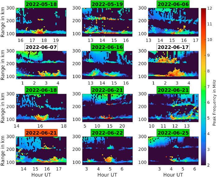
Figure 5. DPS4D range vs. time plots showing the evolution of ${\text{foE}}_s$ for 12 instances where ${\text{foE}}_s$ exceeded 9 MHz.

Figure 6

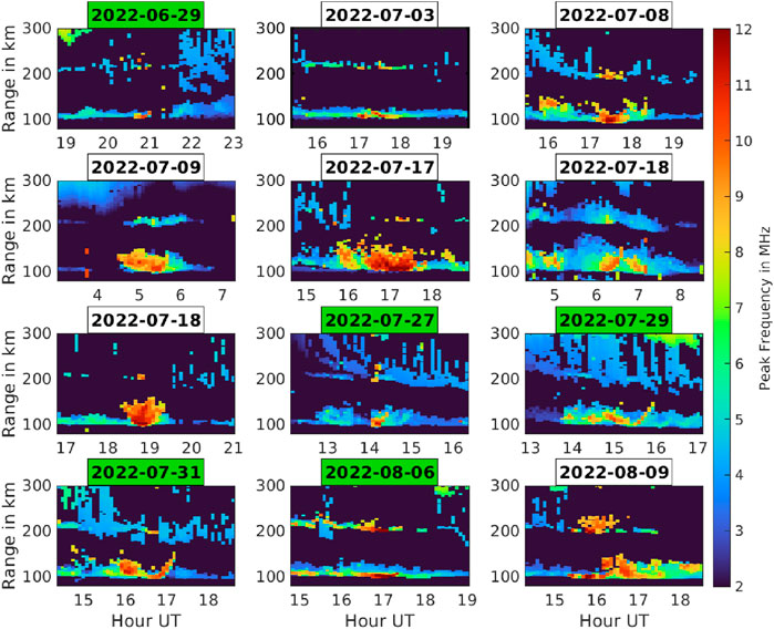
Figure 6. DPS4D range vs. time plots showing the evolution of ${\text{foE}}_s$ for 12 instances where ${\text{foE}}_s$ exceeded 9 MHz.

Upon examination of Figures 5, 6, common features can be observed in many of the intense ${\text{E}}_s$ events. These events typically last for approximately an hour, and ${\text{E}}_s$ is often observed approaching from a higher range and/or departing to a higher range. When both occur, it makes a noticeable “V” shape similar to those observed with VHF radars in Sun et al. (2020) and Patra et al. (2012). Although this pattern is not present in all cases, most instances contain one or multiple “V”s or partial “V”s. Specifically, 20 of the 24 cases (83%) have clear “V” shapes. The four cases where “V” is less clear (2022-05-19, 2022-06-29, 2022-07-03, and 2022-08-06) still have some movement in range but certainly less than the other 20.

Naively, one might assume that the “V” shape is indicative of the vertical movement of ${\text{E}}_s$, and it is certainly well-documented that the height of ${\text{E}}_s$ follows the descending tidal wind shears (Haldoupis et al., 2006), but ${\text{E}}_s$ is not known to move back up in altitude after it descends. Moreover, the timescales here are much too short to be explained by a descending and/or ascending wind shear. We also note that in many cases, the intense ${\text{E}}_s$ is on the top of (or in addition to) a more persistent ${\text{E}}_s$ layer with ${\text{foE}}_s$ above 4 MHz.

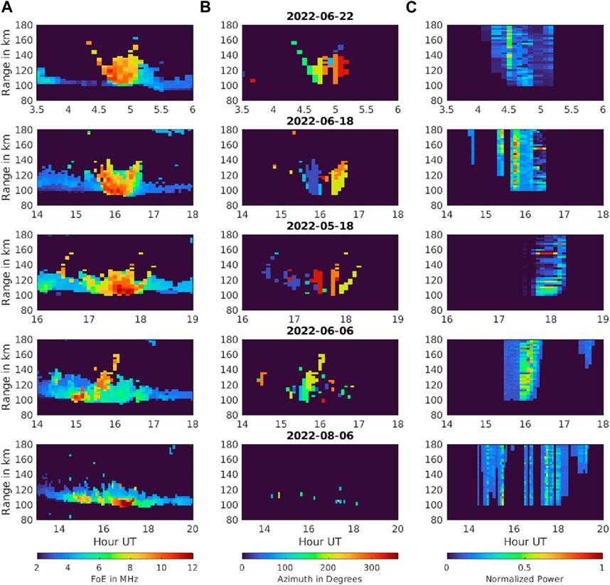
In most of these cases, the azimuthal direction of the intense ${\text{E}}_s$ changes with the approaching and departing features of the “V” structure, indicating movement across the DPS4D field of view. We will now focus on a few cases where intense ${\text{E}}_s$ was present at the same time as LWA observations. Using the LWA’s ${\text{E}}_s$ tracking capability will shed light on the nature of these “V” -shaped structures. We will analyze four cases with a “V” shape and one without. Figure 7 shows all five case studies, where each row of plots represents a different day. The left column shows the RTF plots, and the middle column shows the azimuth plots. Using the geolocated structures measured by the LWA, we can create a similar range vs. time plot, where the normalized LWA-measured power is represented by color. In this plot, the range refers to the distance from the Ft. Stockton DPS4D (assuming a 100 km height). These plots are shown in the right column of Figure 7. We note that since the structures are typically measured at large zenith angles with the LWAs, they are often smeared in range on our plots. Adding more LWA stations to the region will improve the localization. The date, time range, and peak ${\text{foE}}_s$ for each of the five case studies are presented in Table 1. The table also indicates whether a “V” or partial “V” was present and the estimated velocity for each event.

Figure 7

Figure 7. ${\mathrm{E}}_s$ occurring on 22 June 2022, 18 June 2022, 18 May 2022, 6 June 2022, and 6 August 2022 arranged, respectively, from top to bottom. Comparison plots between (A) peak frequency of E layer (foE) as a function of time and range as measured from the Ft Stockton DPS4D; (B) azimuth of the ${\text{E}}_s$ structure, as measured by the Ft. Stockton DPS4D; (C) LWA geolocated ${\text{E}}_s$ structures plotted, shown as a function of time and range from the Ft. Stockton DPS4D.

Table 1

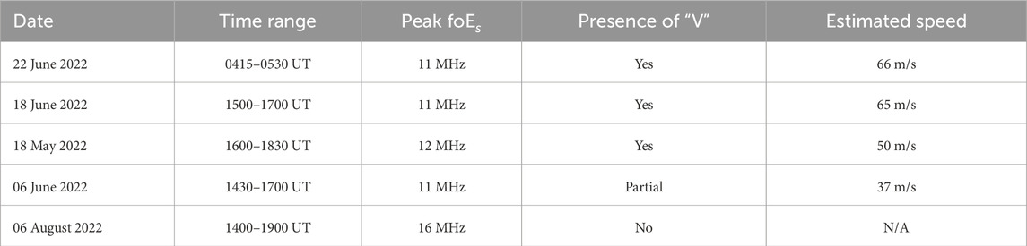
Table 1. Parameters from intense sporadic E events.

In the following subsections, we will discuss the angle of arrival measurements from the DPS4D; however, we note that although the cables used for the DPS4D were phase-matched in the laboratory, no calibration was performed in the field. Moreover, the beam pattern of a four-element array includes many strong side-lobes. Although the small array may be suitable for strong point sources, a spread ${\text{E}}_s$ event may confuse the direction-finding algorithm of the DPS4D. We, therefore, stress that the angle of arrival estimates from the DPS4D are not nearly as accurate as the LWA telescopes, which are each phase calibrated on celestial sources.

3.2.1 22 June 2022

We will first analyze a nighttime ${\text{E}}_s$ event on 22 June 2022. At approximately 0400 UT (2300 LT), LWA-SV identified strong emission coming from the east, and it slowly moved along the horizon toward the south, passing over the Fort Stockton region at approximately 0500 UT (0000 LT). The data from 22 June 2022 are represented in the top row of Figure 7.

The right panel in Figure 7 shows the LWA-measured sky power as a function of time and range from the Ft. Stockton DPS4D. We note that the altitude of the LWA-measured ${\text{E}}_s$ is assumed to be 100 km, which is why the minimum range is roughly 100 km. The left and middle panels of Figure 7 show the DPS4D observations from the same time period. Specifically, the left plot shows ${\text{foE}}_s$ as a function of time and range, and the middle plot shows the measured azimuth of the off-zenith beam measurements. A “V” structure with ${\text{foE}}_s$ near 10 MHz can be observed approaching the DPS4D at approximately 0420 UT (2320 LT). As the ${\text{E}}_s$ structure approaches, the DPS4D first identifies off-zenith returns at a range of $\sim$155 km and azimuth of 150$°$. As time progresses, the returns decrease in range and begin to shift in azimuth. Furthermore, at 0455 UT (2355 LT), the dominant beam for most ranges is directed toward zenith, which is not represented (or rather is represented by 0) in Figure 7. From the plots, we estimate a speed of 66 m/s, assuming that the structure is at an altitude of 100 km and takes $\sim$ 30 min to reach zenith from a distance of 155 km.

Comparing the LWA and DPS4D measurements, we can see that they are measuring the same structure, and both the timing of arrival and departure and the apparent velocity toward the DPS4D are strikingly similar, indicating that they are the same structure. This structure appears to be on top of an existing ${\text{E}}_s$ layer, and is perhaps a modulation of that layer. The ambient ${\text{E}}_s$ layer present for the entire duration of the event is largely coming from zenith. Only the densest structures in the figure are observed in the off-zenith beams.

3.2.2 18 June 2022

On 18 June 2022, a daytime event occurred near 1600 UT (1100 LT). Similar to the 22 June event, the disturbance appears to be a high density modulation superimposed on an existing ${\text{E}}_s$ layer. The second panel from the top row in Figure 7 shows the observations from both the Ft. Stockton DPS4D and the LWA for this day. As shown, a structure observed by the LWA (right plot) approaches the DPS4D starting at approximately 1445 UT (0945 LT) and reaches near zenith at approximately 1600 UT (1100 LT).

As in the case of 22 June, the DPS4D observes a “V” structure that approaches, reaches zenith, and then moves away at a speed of 65 m/s. Again, similar to the case of 22 June, the structure is observed off-zenith and moves from one side of the sky to the other. We note that at 1610 UT (1110 LT), the dominant beam is the one at the zenith, which is not represented in the azimuth plot in Figure 7. Furthermore, the only time an ${\text{E}}_s$ layer is observed by off-zenith beams is during the intense event.

3.2.3 18 May 2022

During this observation, a relatively strong 4–5 MHz ${\text{E}}_s$ layer is observed for the 3 h duration shown in the center row of Figure 7. The DPS4D observes this layer mostly in the zenith beam until $\sim$ 1700 UT (1200 LT), when a “V” structure appears. The structure reaches zenith at approximately 1740 UT (1240 LT) and moves away at an estimated speed of 50 m/s. The DPS4D measurements show that the structure was less dense during its approach than when it was overhead or departing. This may explain why the LWA only observed the structure once it was near zenith or moving away. The structure may have been intensifying as it moved above the Ft. Stockton DPS4D.

3.2.4 6 June 2022

A structure is observed between 1500 and 1630 UT (1000 and 1130 LT). In this case, neither the LWA nor the DPS4D observed the structure’s approach; however, both detected its departure (a partial “V”). The observations shown in the second-to-last row of Figure 7 indicate that the structure mostly formed as it was moving away from the Ft. Stockton area at an apparent speed of 37 m/s. As with the previous cases, the structure appears to be a modulation superimposed on an existing ${\text{E}}_s$ layer. Notably, after the event, a relatively strong (5–6 MHz) range-spread ${\text{E}}_s$ layer persisted until 1700 UT (1200 LT).

3.2.5 6 August 2022

The strong event observed on 6 August 2022 serves as a counterpoint to the overall trend where a moving ${\text{E}}_s$ structure creates a “V” shape in most of the RTF plots of strong Es. The bottom row of Figure 7 shows the observations of the 6 August event. Although it is clear that the LWA co-observed strong ${\text{E}}_s$ with the DPS4D, there is no evidence that it manifests as a moving structure. Little to no “V” shape is present in the DPS4D RTF plot, and similarly, the LWA shows a mostly stationary event.

This event is worth noting because it contained the highest ${\text{foE}}_s$ values observed from the Ft. Stockton DPS4D that summer. The peak foE_s, which occurred near 1700 UT (1200 LT), was over 16 MHz. Furthermore, we note that the LWA plot contains significant gaps in the data, including at the moment where ${\text{foE}}_s$ is the maximum. Upon investigation, it appears that ${\text{E}}_s$ was too stationary and constant in brightness to be flagged in the algorithm described in Section 2.2. As mentioned there, an hour-long median image is subtracted from each 5-min average to remove constant sources of RFI, such as local power lines. This means that if an ${\text{E}}_s$ event is stationary (or moving very slowly) for an hour or more, it will likely not be flagged by the algorithm. Future observing campaigns with additional LWA stations could enable us to remove this restriction and instead rely on anti-coincidence, where multiple stations need to observe ${\text{E}}_s$ for them to be flagged. A new LWA mini-station, with one-quarter as many antennas as a full LWA station, has been built at the north arm of the Very Large Array (Taylor et al., 2025). This new station, LWA-NA, serves as a prototype for future stations that could help monitor ${\text{E}}_s$ in the region.

3.3 E_s and daytime spread F

As mentioned in Section 2.3, an HF receiver was operated at LWA-SV to measure the impacts of ${\text{E}}_s$ on F-layer propagation. Although this receiver was only operational until 6 June, analysis of several early events in the experiment revealed a common trend where the intense ${\text{E}}_s$ events were not only associated with blanketing conditions but also coincided with the presence of spread F. This is notable because the spread F was observed during the day, when it is rarely reported.

3.3.1 18 May 2022

We can first analyze how the oblique ionograms from 18 May 2024 are affected by the passing of the intense sporadic E structure discussed in Section 3.2.3. Since the ${\text{foE}}_s$ of the background ${\text{E}}_s$ layer is approximately 5 MHz, we do not expect to observe dramatic changes to E layer propagation below the 20 MHz upper cutoff of the DPS4D along the oblique link. Using the secant law, a layer with ${\text{foE}}_s$ exceeding 4.4 MHz should allow propagation over 20 MHz. However, we can analyze the impact the cloud has on F-layer propagation.

Figure 8 shows a progression of ionograms made on the oblique link at the time the intense ${\text{E}}_s$ cloud is drifted by the DPS4D on 18 May 2022 at approximately 1730 UT (1230 LT). In addition, the RTF plot from the Ft. Stockton DPS4D is also shown. As the large structure approaches, the oblique reflections exhibit frequency spreading. Interestingly, the primary effect of the intense ${\text{E}}_s$ structure does not appear to simply block (blanket) propagation from the DPS4D. While blanketing conditions are observed in the 1800 UT ionogram, the preceding 30 min show significant spreading along both the O- (left) and X- (right) mode F-layer traces. The F-layer traces are only affected in this way when the intense ${\text{E}}_s$ event is near the oblique propagation path. After approximately 1800 UT (1300 UT) or so, the oblique ionograms return to a non-spread appearance for the rest of the day.

Figure 8

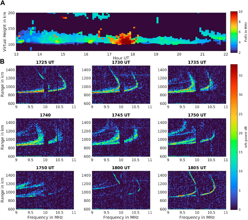
Figure 8. (A) RTF plot from the Ft. Stockton DPS4D on 18 May 2022. (B) [nine panels] Oblique ionograms measured between the Ft. Stockton DPS4D and an HF receiver at LWA-SV. Spread F and blanketing conditions can be observed, coincidingt with the passage of intense E_s.

3.3.2 6 June 2022

Similar to the 18 May event, the 6 June event described in Section 3.2.4 had a distinct ${\text{E}}_s$ structure, which had a noticeable effect on the oblique ionograms. Figure 9 shows the progression of obliques and the RTF plot from 6 June at approximately 1500 UT (1000 LT). As can be observed, the structure appearing in the Ft. Stockton DPS4D is coincident with frequency spreading and blanketing conditions on both the O- and X-mode F-layer traces. After approximately 1730 UT (1230 LT), the spread conditions diminish and the traces go back to their normal non-spread appearance.

Figure 9

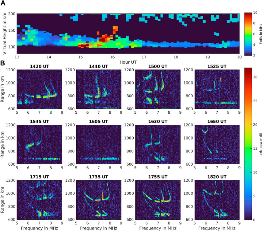
Figure 9. (A) RTF plot from the Ft. Stockton DPS4D on 6 June 2022. (B) [12 panels] Oblique ionograms measured between the Ft. Stockton DPS4D and an HF receiver at LWA-SV. Spread F and blanketing conditions can be observed, coinciding with the passage of intense E_s.

3.3.3 19 May 2022

While the 18 May and 6 June events had a discrete ${\text{E}}_s$ structure, the 19 May events (also shown in Figure 5) are more complex. Multiple partial “V” structures can be observed over a $\sim$5-hour period. In this study, we see again that strong ${\text{E}}_s$ conditions were accompanied by spread F and blanketing conditions for several hours starting at 1300 UT (0800 LT). Figure 10 shows ionograms every 30 min from 1300 to 1830 UT (0800 to 1330 LT) and the RTF plot. As observed, when the severe ${\text{E}}_s$ conditions end near 1700 UT (1200 LT), the spread F conditions also dissipate.

Figure 10

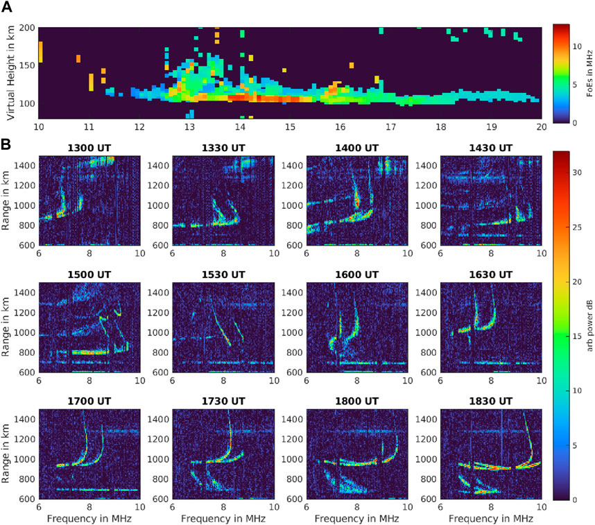
Figure 10. (A) RTF plot from the Ft. Stockton DPS4D on 19 May 2022. (B) [12 panels] Oblique ionograms measured between the Ft. Stockton DPS4D and an HF receiver at LWA-SV. Spread F and blanketing conditions can be observed, coinciding with the occurrence of intense E_s.

3.3.4 7 May 2022

The previous observations utilize the vertical E_s soundings from the Ft. Stockton DPS4D to identify ${\text{E}}_s$, which causes spread F in the oblique (Ft. Stockton to Sevilleta) ionograms. On 7 May, however, an intense ${\text{E}}_s$ event was observed by the LWAs moving directly between Ft. Stockton and Sevilleta. The structure was too small and too far north to be observed by the DPS4D directly, but it had a significant effect on the oblique propagation. Because this event was relatively close to the LWAs and, therefore, was observed at a high zenith angle, they produced very high-resolution maps of its position. The structure was small, likely only a few tens of km across.

Figure 11 shows the geolocation data from both the LWA radio telescopes and the corresponding oblique ionograms from the same time. The red line represents the straight line path between the Ft. Stockton DPS4D and the Sevilleta receiver; the HF propagation can be assumed to follow this path. As shown in the figure, the passage of the intense ${\text{E}}_s$ structure along the oblique propagation path corresponds to a dramatic change in the oblique ionogram. The ionogram at 1625 UT (1125 LT) is typical of a daytime F-layer oblique ionogram. There is really no spread on either the O- or X-mode trace. However, as the structure approaches the propagation path in the 1640 and 1710 UT (1140 and 1210 LT) snapshots, the ionogram begins to display both frequency and range spreading. Finally, at 1725 UT (1225 LT), we see full blanketing conditions when the structure is directly in the path of the oblique propagation.

Figure 11

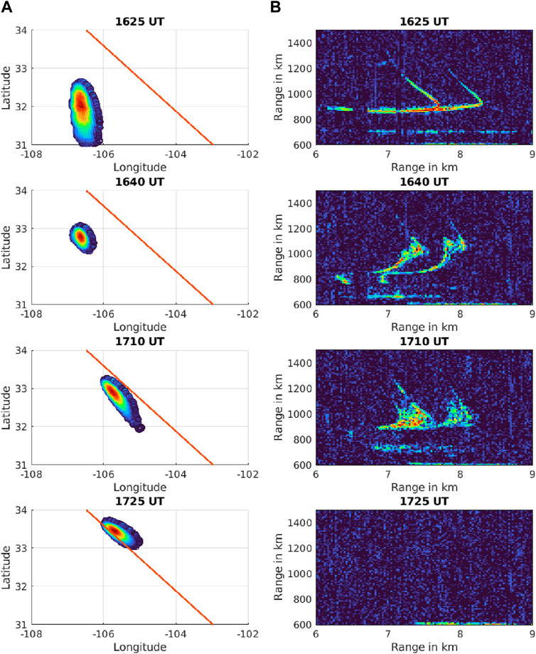
Figure 11. (A) Four snapshots of an intense ${\text{E}}_s$ structure observed by the LWA radio telescopes on 7 May 2022. A line showing the path between the Sevilleta receiver and the Ft. Stockton DPS4D is shown in red. (B) Four corresponding oblique ionograms from the same time.

Since the LWAs imaged the ${\text{E}}_s$ structure with such high resolution, we can estimate a velocity (speed and heading). Based on the four snapshots shown in the figure, the structure is estimated to be traveling with a heading of 30$°$ at a speed of 75 m/s. This is the highest of the speeds reported in this paper, but we should keep in mind that this is the only measurement with a two-dimensional velocity estimate. For the previous events, we could only estimate a one-dimensional speed to and from the DPS4D because the LWA measurements were at too low zenith angles to adequately resolve the positions.

4 Discussion

The cases of intense ${\text{E}}_s$ presented in this study display characteristics of a highly structured, perhaps turbulent, plasma. LWA observations of moving ${\text{E}}_s$ structures show that the “V” shapes measured by the DPS4D at Ft. Stockton are relatively small regions of intense E_s. As shown in Figures 5, 6, the vast majority of cases of strong ${\text{E}}_s$ (${\text{foE}}_s>$ 9 MHz) had at least part of a “V” shape present, indicating off-zenith backscatter from an approaching and/or departing ${\text{E}}_s$ structure. These “V” structures are not consistent with a thin, dense layer producing a glassy mirror-like reflection directly above the DPS4D. Such a glassy layer would manifest at a single range without spread. Range-spread ${\text{E}}_s$ is indicative of a plasma with a significant structure in three dimensions. Although this is a trend, it is not a general rule. A good example of an exception to the “V” shape can be found in Figure 6 during the 2022-08-06 event. Almost no E layer range spreading is observed in this example despite the very high ${\text{foE}}_s$ values observed.

Comparing VHF coherent scatter measurements of ${\text{E}}_s$ with Digisonde measurements, Hussey et al. (1998) noted that range-spread echoes in ionosondes were likely caused by a corrugated vertical structure, which allows for off-zenith range spread echoes. This corrugation may be evident in Figures 5, 6. For instance, within the “V” shapes on 2022-06-16, 2022-07-08, and 2022-07-17, clear striations can be observed in the approaching structure. Separations of the striations are on the order of just a few 5-min integrations, which is consistent with acoustic-gravity waves in the mesopause region. Longer period oscillations of 30 min or more are evident on 2022-06-07, 2022-06-16, 2022-06-21, 2022-07-18, and 2022-07-29. The periods observed in this study are consistent with typical gravity wave periods.

Alternatively, the corrugation responsible for the off-zenith backscatter (spread ${\text{E}}_s$) could be occurring on much shorter periods. For instance, the KH billow structures shown in Hysell et al. (2012) have periods of a few tens of seconds rather than minutes. The gravity wave timescale periods observed in Figures 5, 6 may simply imply that gravity waves modulate or even trigger KH instability that forms the small-scale structures.

The “V”-shaped structures reported in this study are strikingly similar to those observed by the VHF radars in Patra et al. (2012) and Sun et al. (2020). While these two examples are from VHF observations, it is possible that mid-latitude stations of the Super Dual Auroral Radar Network (SuperDARN) also detect backscatter from intense ${\text{E}}_s$ events in the HF band (Kunduri et al., 202). It is important to note that the backscatter presented in this study and Patra et al. (2012), Sun et al. (2020), and Kunduri et al. (2023) is not caused by coherent field-aligned structures. These are simply ruled out by the geometry of the radar $\vec{k}$ vectors with respect to the geomagnetic field. Instead, the radar returns are likely coming from regions of a plasma (perhaps overdense) with significantly sufficient structure in three dimensions to enable backscatter at high zenith angles.

The daytime events described by Patra et al. (2012) and Sun et al. (2020) were also coincident with the scintillation of trans-ionospheric RF links. Although no scintillation receivers were deployed during our experiment, spread F conditions were observed to be associated with the ${\text{E}}_s$ structures. This is significant because the four events described in Section 3.3 occurred during the daytime. Normally, spread-F and scintillation are associated with the nighttime phenomenon. For instance, equatorial spread F (ESF) is caused by equatorial plasma bubbles, where strong deletions produce small-scale irregularities in the nighttime ionospheric F-layer (Woodman, 2009; Huba, 2023). During geomagnetic storm enhancements, ESF can also reach the mid-latitudes (Martinis et al., 2015). As mentioned in the introduction, mid-latitude spread-F is also associated with nighttime sporadic E events responsible for coherent backscatter at VHF frequencies (Tsunoda and Cosgrove, 2001; Haldoupis et al., 2003).

The daytime mid-latitude spread F presented in this study, however, was not caused by these exclusively nighttime events. Assuming that daytime ${\text{E}}_s$ is not electrically coupled to the F layer (as it is at night), we hypothesize that plasma irregularities within the intense ${\text{E}}_s$ may act simply as a scattering screen for waves propagating to the F layer. This may be a simpler solution than trying to explain any daytime irregularities in the F layer itself. The ${\text{E}}_s$ coincident scintillation observations of Sun et al. (2020) and others already imply that a small-scale structure is present within intense E_s. For the 540 km oblique path from Ft. Stockton to Sevilleta, the maximum Fresnel zone is approximately 2 km at 5 MHz. So, we can assume that any E-layer irregularities smaller than 2 km would produce spreading on the F-layer trace. As soon as the intense ${\text{E}}_s$ structure has passed, the observations show that the F-layer traces go back to their typical non-spread appearance. This quick change is consistent with the phase screen hypothesis.

As discussed in the introduction, KH instabilities almost certainly occur within ${\text{E}}_s$ layers. The observations presented in this study and Obenberger et al. (2021) show highly localized (a few tens of km) ${\text{E}}_s$ structures that are consistent with KH billow scale sizes. It is plausible that the turbulent plasma found in KH billows, with vertical scale sizes of a few km (Hysell et al., 2012), could produce the off-zenith backscatter and spread F observed during this study. A full-wave modeling approach, however, should be employed in a future study to confirm that such a mechanism is probable.

Although the majority of the observations presented in this study are too close to the horizon to resolve any front-like shapes, Obenberger et al. (2021) showed that the LWA observed structures that are observed at higher elevation angles are often front-like, similar to the GNSS tomography observations reported by Maeda and Heki (2014). Furthermore, the tens of m/s velocities measured by Obenberger et al. (2021) and this study are consistent with GNSS tomography observations. It is possible that the structures reported in this study and those reported by Maeda and Heki (2014) (and subsequent studies) are caused by KH billows or Ekman spirals. Fortunately, a sufficient number of GNSS receivers were co-located with the observations made by Sun et al. (2020), and not surprisingly, a strong ${\text{E}}_s$ front was detected to be coincident with the “V”-shaped structure observed by the VHF radar front.

The structures reported in Maeda and Heki (2014), Patra et al. (2012), Sun et al. (2020), and in this study may be a more general version of the irregularities that trigger the FAIs associated with QP echoes. Comparing the observations of QP echoes with GNSS tomography or a passive VHF system, such as the LWA, would be beneficial for understanding this mechanism. There may be other sources of turbulence within ${\text{E}}_s$ plasma contributing to the observations presented in this study, but a wind shear instability, such as the KH instability, is already known to modulate ${\text{E}}_s$ regularly and is, therefore, a reasonable candidate. Future ${\text{E}}_s$ campaigns would benefit from multi-instrument suites. Combining ionosondes with radio telescopes, VHF radars, GNSS arrays, and in situ rocket payloads would be greatly advantageous.

It is not particularly surprising that ${\text{E}}_s$ could exhibit high levels of turbulence. However, it may be a slight surprise that 20 of the 24 cases of intense ($>$ 9 MHz) ${\text{E}}_s$ measured in this study could be characterized as turbulent. When referring to a turbulent plasma, ${\text{foE}}_s$ may take on a new meaning. Rather than describing “the” plasma frequency, ${\text{foE}}_s$ of a turbulent ${\text{E}}_s$ layer is really describing the highest frequency observably scattered from a highly variable plasma. This could be described as a frequency-dependent radar cross-section, which is likely related to a spectrum of plasma densities found within a ${\text{E}}_s$ structure. This may be convenient for modeling intense or blanketing sporadic E layers as it appears that most cases could be described as turbulent. The typical wind shear model for describing ${\text{E}}_s$ may not need to invoke thin, glassy layers with uniform frequencies exceeding 9 MHz.

Finally, it is worth discussing exactly what the LWA is observing. Obenberger et al. (2021) concluded that at least some of the emissions detected by the LWA had to originate from broadband RFI generated by devices connected to the electrical grid. This type of RFI is often detected coming from noisy power lines and their components, such as transformers. It is worth questioning, however, whether this is the only source. Platonov and Fleishman (2002) described how a turbulent plasma can radiate broadband RF when suprathermal electrons are present through a process called resonant transition radiation (RTR). In this study, suprathermal electrons with energies on the order of an eV radiate RF as they pass through the regions of changing electron density. Another possibility is that Langmuir waves might be generated and potentially converted to electromagnetic emission. Oppenheim and Dimant (2016) showed that photoelectrons can trigger a bump-on-tail instability in the F1 layer to produce 150 km echoes, often observed by powerful VHF radars perpendicular to the geomagnetic field.

An example of HF/VHF emissions in the E region may have already been found; Obenberger et al. (2014b) and later works have shown that large meteors can produce a broadband glow. Furthermore, Obenberger et al. (2020) examined how anion oxidation could produce a spectrum of suprathermal electrons capable of radiating RTR in a turbulent plasma or possibly even generating Langmuir waves. Given that turbulent ${\text{E}}_s$ is now associated with LWA measurements, it is quite possible that some of the emissions observed by the LWA are indeed E_s-related emissions. Given the ubiquity of the electrical grid in North America, it may be difficult to test such a hypothesis with current LWA capabilities. A similar instrument, however, if built on a remote island, could possibly ascertain the answer.

5 Conclusion

In this study, we presented coincident observations of ${\text{E}}_s$ from a DPS4D and the LWA radio telescopes. We find that the LWA telescopes are accurate and reliable tools for geolocating Es. Additionally, we have shown that the intense ${\text{E}}_s$ events (${\text{foE}}_s>$ 9 MHz) occurring near the border between New Mexico and Texas during the summer of 2022 typically created significant off-zenith scatter in the DPS4D ionograms. RTF plots reveal that these events exhibit a “V” pattern, where the intense ${\text{E}}_s$ event is often detected approaching and departing from the field of view of the DPS4D at speeds of a few tens of m/s. Comparisons with LWA observations reveal that these are discrete regions of intense ${\text{E}}_s$ that move through regions of pre-existing, less dense E_s. The off-zenith backscatter, along with the observations of ${\text{E}}_s$-induced daytime spread F, indicate the presence of significant, perhaps turbulent, structures. Context provided by other recent literature on intense ${\text{E}}_s$ suggests that many of these high-density events are the result of neutral instabilities such as KH billows or Ekman spirals.

Data availability statement

The raw data supporting the conclusions of this article will be made available by the authors, without undue reservation.

Author contributions

KO: conceptualization, data curation, formal analysis, funding acquisition, investigation, methodology, project administration, resources, software, supervision, validation, visualization, and writing – original draft. CA: data curation, formal analysis, software, and writing – review and editing. JC: conceptualization, funding acquisition, supervision, and writing – review and editing. ED: conceptualization, data curation, formal analysis, resources, software, and writing – review and editing. JD: data curation, resources, software, and writing – review and editing. JE: conceptualization and writing – review and editing. DE: conceptualization and writing – review and editing. CF: formal analysis, funding acquisition, supervision, validation, and writing – review and editing. JH: funding acquisition, resources, supervision, validation, and writing – review and editing. GT: conceptualization, funding acquisition, resources, supervision, and writing – review and editing.

Funding

The author(s) declare that financial support was received for the research and/or publication of this article. This research was funded by the NASA Space Weather Science Applications Operations 2 Research program under Grant 20-SWO2R20-2-0007. This research was also sponsored in part by the Air Force Office of Scientific Research (AFOSR) Lab Task 23RVCOR002.

Acknowledgments

The authors thank referees for their insightful comments. The authors would like to thank Mickey Perry and Pecos County, Texas, for allowing AFRL to deploy a DPS4D on country property. The authors would also like to thank Dwayne Bonham and Benny Walker of the Pecos County Amateur Radio Club for assistance during the experiment.

Conflict of interest

Author CT was employed by the Fourth State Communications.

The remaining authors declare that the research was conducted in the absence of any commercial or financial relationships that could be construed as a potential conflict of interest.

Generative AI statement

The author(s) declare that no Generative AI was used in the creation of this manuscript.

Publisher’s note

All claims expressed in this article are solely those of the authors and do not necessarily represent those of their affiliated organizations, or those of the publisher, the editors and the reviewers. Any product that may be evaluated in this article, or claim that may be made by its manufacturer, is not guaranteed or endorsed by the publisher.

Author disclaimer

The views expressed are those of the authors and do not reflect the official guidance or position of the United States Government, the Department of Defense, or of the United States Air Force. The appearance of external hyperlinks does not constitute endorsement by the United States Department of Defense (DoD) of the linked websites, or the information, products, or services contained therein. The DoD does not exercise any editorial, security, or other control over the information you may find at these locations.

References

Bernhardt, P. A. (2002). The modulation of sporadic-e layers by kelvin–helmholtz billows in the neutral atmosphere. J. Atmos. Solar-Terrestrial Phys. 64, 1487–1504. doi:10.1016/S1364-6826(02)00086-X

CrossRef Full Text | Google Scholar

Bui, M. X., Hysell, D. L., and Larsen, M. F. (2023). Midlatitude sporadic e-layer horizontal structuring modulated by neutral instability and mixing in the lower thermosphere. J. Geophys. Res. Space Phys. 128, e2022JA030929. doi:10.1029/2022JA030929

CrossRef Full Text | Google Scholar

Chu, Y.-H., and Wang, C.-Y. (1997). Interferometry observations of three-dimensional spatial structures of sporadic e irregularities using the chung-li vhf radar. Radio Sci. 32, 817–832. doi:10.1029/96RS03578

CrossRef Full Text | Google Scholar

Cranmer, M. D., Barsdell, B. R., Price, D. C., Dowell, J., Garsden, H., Dike, V., et al. (2017). Bifrost: a python/c++ framework for high-throughput stream processing in astronomy. J. Astronomical Instrum. 06, 1750007. doi:10.1142/S2251171717500076

CrossRef Full Text | Google Scholar

Ejiri, M. K., Nakamura, T., Tsuda, T. T., Nishiyama, T., Abo, M., Takahashi, T., et al. (2019). Vertical fine structure and time evolution of plasma irregularities in the es layer observed by a high-resolution ca+ lidar. Earth Planets Space 3, 3. doi:10.1186/s40623-019-0984-z

CrossRef Full Text | Google Scholar

Ellingson, S. W., Taylor, G. B., Craig, J., Hartman, J., Dowell, J., Wolfe, C. N., et al. (2013). The lwa1 radio telescope. IEEE Trans. Antennas Propag. 61, 2540–2549. doi:10.1109/TAP.2013.2242826

CrossRef Full Text | Google Scholar

Haldoupis, C., Kelley, M. C., Hussey, G. C., and Shalimov, S. (2003). Role of unstable sporadic-e layers in the generation of midlatitude spread f. J. Geophys. Res. Space Phys. 108. doi:10.1029/2003JA009956

CrossRef Full Text | Google Scholar

Haldoupis, C., Meek, C., Christakis, N., Pancheva, D., and Bourdillon, A. (2006). Ionogram height–time–intensity observations of descending sporadic e layers at mid-latitude. J. Atmos. solar-terrestrial Phys. 68, 539–557. doi:10.1016/j.jastp.2005.03.020

CrossRef Full Text | Google Scholar

Hu, L., Yue, X., and Ning, B. (2017). Development of the beidou ionospheric observation network in China for space weather monitoring. Space weather. 15, 974–984. doi:10.1002/2017SW001636

CrossRef Full Text | Google Scholar

Huba, J. D. (2023). Resolution of the equatorial spread f problem: revisited. Front. Astronomy Space Sci. 9. doi:10.3389/fspas.2022.1098083

CrossRef Full Text | Google Scholar

Hussey, G. C., Schlegel, K., and Haldoupis, C. (1998). Simultaneous 50-mhz coherent backscatter and digital ionosonde observations in the midlatitude e region. J. Geophys. Res. Space Phys. 103, 6991–7001. doi:10.1029/97JA03089

CrossRef Full Text | Google Scholar

Hysell, D. L., and Burcham, J. D. (2000). The 30-mhz radar interferometer studies of midlatitude e region irregularities. J. Geophys. Res. Space Phys. 105, 12797–12812. doi:10.1029/1999JA000411

CrossRef Full Text | Google Scholar

Hysell, D. L., and Larsen, M. F. (2021). Vhf imaging radar observations and theory of banded midlatitude sporadic e ionization layers. J. Geophys. Res. Space Phys. 126, e2021JA029257. doi:10.1029/2021JA029257

CrossRef Full Text | Google Scholar

Hysell, D. L., Nossa, E., Larsen, M. F., Munro, J., Smith, S., Sulzer, M. P., et al. (2012). Dynamic instability in the lower thermosphere inferred from irregular sporadic e layers. J. Geophys. Res. Space Phys. 117. doi:10.1029/2012JA017910

CrossRef Full Text | Google Scholar

Hysell, D. L., Nossa, E., Larsen, M. F., Munro, J., Sulzer, M. P., and González, S. A. (2009). Sporadic e layer observations over arecibo using coherent and incoherent scatter radar: Assessing dynamic stability in the lower thermosphere. J. Geophys. Res. Space Phys. 114. doi:10.1029/2009JA014403

CrossRef Full Text | Google Scholar

Kunduri, B. S. R., Erickson, P. J., Baker, J. B. H., Ruohoniemi, J. M., Galkin, I. A., and Sterne, K. T. (2023). Dynamics of mid-latitude sporadic-e and its impact on hf propagation in the north american sector. J. Geophys. Res. Space Phys. 128. doi:10.1029/2023JA031455

CrossRef Full Text | Google Scholar

Larsen, M. F. (2000). A shear instability seeding mechanism for quasiperiodic radar echoes. J. Geophys. Res. Space Phys. 105, 24931–24940. doi:10.1029/1990

CrossRef Full Text | Google Scholar

Maeda, J., and Heki, K. (2014). Two-dimensional observations of midlatitude sporadic e irregularities with a dense gps array in japan. Radio Sci. 49, 28–35. doi:10.1002/2013RS005295

CrossRef Full Text | Google Scholar

Maeda, J., and Heki, K. (2015). Morphology and dynamics of daytime mid-latitude sporadic-e patches revealed by gps total electron content observations in Japan. Earth Planets Space 67, 89. doi:10.1186/s40623-015-0257-4

CrossRef Full Text | Google Scholar

Martinis, C., Baumgardner, J., Mendillo, M., Wroten, J., Coster, A., and Paxton, L. (2015). The night when the auroral and equatorial ionospheres converged. J. Geophys. Res. Space Phys. 120, 8085–8095. doi:10.1002/2015JA021555

CrossRef Full Text | Google Scholar

Obenberger, K., Taylor, G., Hartman, J., Clarke, T., Dowell, J., Dubois, A., et al. (2015). Monitoring the sky with the prototype all-sky imager on the lwa1. J. Astronomical Instrum. 04, 1550004. doi:10.1142/S225117171550004X

CrossRef Full Text | Google Scholar

Obenberger, K. S., Dowell, J., Fallen, C. T., Holmes, J. M., Taylor, G. B., and Varghese, S. S. (2021). Using broadband radio noise from power-lines to map and track dense E_s structures. Radio Sci. 56, e2020RS007169. doi:10.1029/2020RS007169

CrossRef Full Text | Google Scholar

Obenberger, K. S., Dugick, F. K. D., and Bowman, D. C. (2023). Remote sensing small explosives with an ionospheric radar. Earth Space Sci. 10, e2022EA002737. doi:10.1029/2022EA002737

CrossRef Full Text | Google Scholar

Obenberger, K. S., Holmes, J. M., Ard, S. G., Dowell, J., Shuman, N. S., Taylor, G. B., et al. (2020). Association between meteor radio afterglows and optical persistent trains. J. Geophys. Res. Space Phys. 125, e2020JA028053. doi:10.1029/2020JA028053

CrossRef Full Text | Google Scholar

Obenberger, K. S., Taylor, G. B., Hartman, J. M., Dowell, J., Ellingson, S. W., Helmboldt, J. F., et al. (2014b). Detection of radio emission from fireballs. Astrophysical J. 788, L26. doi:10.1088/2041-8205/788/2/l26

CrossRef Full Text | Google Scholar

Oppenheim, M. M., and Dimant, Y. S. (2016). Photoelectron-induced waves: a likely source of 150 km radar echoes and enhanced electron modes. Geophys. Res. Lett. 43, 3637–3644. doi:10.1002/2016GL068179

CrossRef Full Text | Google Scholar

Patra, A. K., Chaitanya, P. P., and Bhattacharyya, A. (2012). On the nature of radar backscatter and 250 MHz scintillation linked with an intense daytime E_s patch. J. Geophys. Res. Space Phys. 117. doi:10.1029/2011JA016981

CrossRef Full Text | Google Scholar

Platonov, K. Y., and Fleishman, G. D. (2002). Transition radiation in media with random inhomogeneities. Physics-Uspekhi 45, 235–291. doi:10.1070/pu2002v045n03abeh000952

CrossRef Full Text | Google Scholar

Reinisch, B. W., Galkin, I. A., Khmyrov, G. M., Kozlov, A. V., Bibl, K., Lisysyan, I. A., et al. (2009). New digisonde for research and monitoring applications. Radio Sci. 44. doi:10.1029/2008RS004115

CrossRef Full Text | Google Scholar

Reinisch, B. W., Galkin, I. A., Khmyrov, G. M., Kozlov, A. V., Lisysyan, I. A., Bibl, K., et al. (2008). Advancing digisonde technology: the dps-4d. AIP Conf. Proc. 974, 127–143. doi:10.1063/1.2885022

CrossRef Full Text | Google Scholar

Saito, S., Yamamoto, M., Hashiguchi, H., and Maegawa, A. (2006). Observation of three-dimensional structures of quasi-periodic echoes associated with mid-latitude sporadic-e layers by mu radar ultra-multi-channel system. Geophys. Res. Lett. 33. doi:10.1029/2005GL025526

CrossRef Full Text | Google Scholar

Sun, W., Ning, B., Hu, L., Yue, X., Zhao, X., Lan, J., et al. (2020). The evolution of complex E_s observed by multi instruments over low-latitude China. J. Geophys. Res. Space Phys. 125, e2019JA027656. doi:10.1029/2019JA027656

CrossRef Full Text | Google Scholar

Sun, W., Ning, B., Yue, X., Li, G., Hu, L., Chang, S., et al. (2018). Strong sporadic e occurrence detected by ground-based gnss. J. Geophys. Res. Space Phys. 123, 3050–3062. doi:10.1002/2017JA025133

CrossRef Full Text | Google Scholar

Taylor, C. A., Dowell, J., Taylor, G. B., Obenberger, K. S., Chastain, S. I., Verastegui, J., et al. (2025). Design and commissioning of an lwa swarm station: the long wavelength array – north arm. Journal of Astronomical Instrumentation under review.

Google Scholar

Tsunoda, R. T., and Cosgrove, R. B. (2001). Coupled electrodynamics in the nighttime midlatitude ionosphere. Geophys. Res. Lett. 28, 4171–4174. doi:10.1029/2001GL013245

CrossRef Full Text | Google Scholar

Varghese, S. S., Dowell, J., Obenberger, K. S., Taylor, G. B., and Malins, J. (2021). Broadband imaging to study the spectral distribution of meteor radio afterglows. J. Geophys. Res. Space Phys. 126, e2021JA029296. doi:10.1029/2021JA029296

CrossRef Full Text | Google Scholar

Woodman, R. F. (2009). Spread f – an old equatorial aeronomy problem finally resolved? Ann. Geophys. 27, 1915–1934. doi:10.5194/angeo-27-1915-2009

CrossRef Full Text | Google Scholar

Yamamoto, M., Komoda, N., Fukao, S., Tsunoda, R. T., Ogawa, T., and Tsuda, T. (1994). Spatial structure of the e region field-aligned irregularities revealed by the mu radar. Radio Sci. 29, 337–347. doi:10.1029/93RS01846

CrossRef Full Text | Google Scholar