A novel theoretical approach to predict the interannual variability of sulfur in Mercury’s exosphere and subsurface

The surfaces of airless bodies are constantly weathered by ions, meteoroids, and radiation, leading to the ejection of surface atoms to form a tenuous, collisionless atmosphere around the body. In the case of Mercury, its high surface temperatures can also lead to thermal desorption (TD) of atoms. Since its discovery approximately 50 years ago, Mercury’s exosphere has been extensively observed by both ground-based and space-borne telescopes. The MErcury Surface, Space ENvironment, GEochemistry, and Ranging (MESSENGER) spacecraft operated 4 years in orbit around Mercury and allowed for the surface composition species to be inferred, notably including sulfur (S). Sulfur was, however, never observed in Mercury’s exosphere. In this study, we use a unique theoretical approach that combines modeling methods across different dimensional scales to understand the presence of sulfur on Mercury. Using a 3D exospheric global model with a Monte-Carlo test-particles approach and accounting for species diffusion in the first meter of Mercury’s regolith, this study aims to provide the first global prediction of the interannual variability of neutral sulfur density in both Mercury’s exosphere and subsurface. Our model predicts the formation of subsurface reservoirs at different depths according to the planetary longitude, with an equatorial reservoir peak location at ∼ 21 cm and ∼ 8 cm below the surface at the hot and cold poles, respectively. Cold longitudes are also predicted to accumulate 6.7 times more sulfur than the hot longitudes. Regarding the exosphere, the larger abundance of sulfur at the cold longitudes induces a local enhancement of the exospheric density around aphelion. The calcium surface abundance is predicted to influence the sulfur adsorption location, leading to a sulfur content enhancement in the vicinity of the −90°E longitude. Our results could be beneficial for optimizing the planning and aiding the analysis and interpretation of future observations of Mercury’s exosphere by BepiColombo.

1 Introduction

Mercury is an airless body that possesses a tenuous, collisionless atmosphere formed via different weathering mechanisms. This leaves its surface vulnerable to photons, solar wind ions, and micro-meteoroids impacts, all of which can eject atoms from the planet’s surface into its atmosphere (Leblanc and Johnson, 2003; Killen et al., 2007; Cassidy et al., 2015; Killen et al., 2022). Additionally, since Mercury’s surface experiences temperatures as high as ∼700 K on the dayside (Morrison, 1970; Chase et al., 1976), atoms can also thermally desorb from the surface (Yakshinskiy et al., 2000; Leblanc and Johnson, 2003). These four different ejection processes (photon-stimulated desorption (PSD), solar wind sputtering (SWS), micro-meteoroid impact vaporization (MMIV), and thermal-stimulated desorption (TD)) are currently considered the main sources forming the Hermean surface-bound exosphere (Leblanc and Johnson, 2010). Their relative efficiencies depend on the geographical and orbital position of the planet and the binding energy of the ejected atom being considered. This surface binding energy (SBE) is highly dependent on the bond strengths and, thus, the mineral type in which the atom is contained (Morrissey et al., 2022a).

Since the discovery of atoms being ejected from Mercury’s surface and forming a tenuous atmosphere around the planet, Mercury’s surface–exosphere interface has been extensively observed by both ground-based and space-borne telescopes (Broadfoot et al., 1976; Potter and Morgan, 1985). Between 2007 and 2009, the MErcury Surface, Space ENvironment, GEochemistry, and Ranging (MESSENGER) spacecraft performed three fly-bys of Mercury followed by 4 years in orbit around it. This mission allowed for the inference of Mercury’s surface composition, which notably includes some moderately volatile species such as sodium, potassium, and sulfur (S) (Nittler et al., 2018). Although the former were clearly identified in Mercury’s exosphere, sulfur has never been observed in its neutral form (Cassidy et al., 2015; Lierle et al., 2022). This lack of observation is possibly due to the low photon scattering probability (g value) of sulfur (Killen et al., 2009). MESSENGER surface abundance maps revealed that the distribution of sulfur is highly non-uniform, with higher S abundance in a localized patch of the northern hemisphere (Nittler et al., 2018). Moreover, recent studies suggest that the hollows, geological formations observed mostly in crater-related units, could potentially be formed by local sulfur accumulation (Phillips et al., 2021; Barraud et al., 2023). This suggests that sulfur should be present in both the surface and the exosphere of Mercury, with atomic migration and/or diffusion processes that could be key to sustaining such geological features. However, more research is needed to better understand the physics underlying these migration processes for S.

Mercury’s continuous bombardment by micro-meteoroids has fractured the surface into very fine grains. The resulting regolith is formed via packing of these fine grains (mean size ∼50 µm) (Wurz and Lammer, 2003) and is considered to be highly porous (≥85%), similar to the Moon (McKay and Ming, 1990; McKay et al., 1991). As atoms are deposited on Mercury’s surface, this porous structure becomes more favorable for subsurface diffusion via successive adsorption and desorption from grain to grain (Sprague, 1990; Killen and Morgan, 1993; Teolis et al., 2023). Given sufficient time, this grain-to-grain migration could lead to a net diffusion in the subsurface, similar to what was suggested by Reiss et al. (2021) regarding the Moon. These atoms can eventually be retained efficiently in the regolith if the local ejection efficiencies of the different processes become negligible compared to the SBE of the atom. Such regions are mostly located at depth (Verkercke et al., 2024), where the atoms are protected from PSD, SWS, and MMIV and where the temperature is lower with respect to the SBE of the atoms. At these locations, the adsorbates can accumulate to form a reservoir. As the temperature is depth-dependent, colder longitudes will form shallower reservoirs of adsorbed atoms than hotter longitudes. However, some large uncertainties still exist regarding the SBE distribution of many Mercury species, stressing the need for more MD computations (Killen et al., 2022; Morrissey et al., 2022b; Morrissey et al., 2025). Nevertheless, subsurface volatile reservoirs have been invoked to explain the nature of geomorphological surface features as low-reflectance materials (LRMs, Lark et al., 2023), including hollows (i.e., flat-floored, shallow, and bright depressions) (Barraud et al., 2023). The latter are correlated with impact craters, which suggests that impacts are needed to expose buried volatiles (Thomas et al., 2014; Blewett et al., 2016) or increase the local temperature enough to drive devolatilization of a reservoir (Phillips et al., 2021; Munaretto et al., 2023).

This study presents and discusses the first global prediction of the interannual variability of neutral sulfur density in both Mercury’s exosphere and subsurface using a novel modeling approach connecting dimensional scales from the atomic scale to the global exosphere scale. This approach has been suggested by many previous researchers but has not yet been conducted in a single study (Morrissey et al., 2021; Killen et al., 2022). At the global/granular scales, we use a 3D exospheric global model (3D EGM) with a Monte-Carlo test-particle approach, accounting for species diffusion in the first meter of Mercury’s regolith. In particular, we investigate the dependence of the sulfur content in the exosphere and surface on the major desorption processes operating on airless bodies and discuss these in the context of the future analysis of Mercury’s surface and exosphere by the BepiColombo mission. The surface and subsurface adsorption and desorption of sulfur on Mercury are then constrained using the large-scale atomic/molecular massively parallel simulator (LAMMPS) (Plimpton, 1995) molecular dynamics (MD) tool to compute the SBE of sulfur on different substrates typically found on Mercury, such as SiO₂, Na, and Ca. Such an approach for SBE calculation has been validated for other volatile substrates (Morrissey et al., 2025). The surface abundance maps derived from MESSENGER XRS instruments are used to constrain the exospheric model as realistically as possible. The MD modeling of sulfur absorption on different substrates and the parameterization and the description of the 3D EGM and subsurface diffusion are described in Section 2. Section 3 presents the analysis and comparison of different scenarios, and Section 4 summarizes the conclusions of this study.

2 Atomic to planetary scale modeling

This section describes the different models used in this study, starting with the MD representation of different substrates at the atomic scale and the SBE computation of sulfur on these surfaces. The second part describes the 3D EGM and its parameters.

2.1 Molecular dynamic simulations

MD is a numerical simulation tool that can be used to compute time-integrated movements of atoms/molecules in a slab of substrate representing a grain of Mercury’s regolith. The simulation starts with the initial positions and velocities of all the atoms attributed accordingly to the crystal lattice of the substrate. Atomic interactions are computed according to an inter-atomic potential that defines the different forces between neighboring atoms. The equations of motion are then used to compute and update the atoms’ positions and velocities at every time step (van Duin et al., 2001; van Duin et al., 2003; Aktulga et al., 2012). Following the methodology of Morrissey et al. (2025), once the substrates are equilibrated to the desired temperature, a single atom is created above the grain’s surface to study its adsorption. If the atom adsorbs, the SBE is computed for this atom. The SBE is defined as the energy needed in the direction normal to the surface to completely remove an atom so that it no longer interacts with the substrate. The inter-atomic interactions are all described using a reactive force field (ReaxFF) inter-atomic potential implemented in LAMMPS. ReaxFF was first introduced by van Duin et al. (2001) and is capable of dynamically capturing bonded and non-bonded interactions within the system. In our study, the ReaxFF potential is directly adopted from Psofogiannakis et al. (2015). The potential used in this study was developed by merging and expanding previously tested and published ReaxFF force fields used in the study of Si-O-, Na-, Ca-, and S-bearing systems (van Duin et al., 2003; Ojwang et al., 2008; Psofogiannakis et al., 2015).

The three substrates chosen to explore S adsorption were SiO₂, Na, and Ca. SiO₂ is one of the main components of Mercury’s surface (Nittler et al., 2018; Renggli et al., 2022), comprising approximately half of its regolith composition, suggesting that the majority of the volatiles would likely adsorb onto a SiO₂ surface. However, Renggli et al. (2022) showed through laboratory experiments on Mercury surface analogs that at high temperatures, the substrate can form a natural coating of Ca/Mg/Fe, on which sulfur would preferentially deposit rather than on silicates. This motivates our choice for the Ca crystal surface, a conclusion that is supported by MESSENGER’s observations of the distribution of elemental compositions (Nittler et al., 2018). The Na crystal serves as a reference for another volatile present on Mercury that was also studied by Renggli et al. (2022) and was found to have a weak affinity for S deposition.

To build the SiO₂ surface, the unit cell was replicated eight times along the x and y dimensions (the sides of the simulation box) and four times along the vertical z-axis to create a bulk crystal with a volume of 39.5 × 34.2 × 22.2 ų (Ogata et al., 1987). Periodic boundary conditions were used in each direction, thus removing boundary effects and simulating an infinite bulk (Morrissey et al., 2022b). The density of this bulk sample was approximately 2.6 g/cm³, which agreed well with experimental values (Haynes, 2014). Similar to previous studies (Baudin et al., 1997; Morrissey et al., 2022a), the simulated sample was heated to 100 K at constant pressure (0 atm) and constant particle number for 5 ps (NPT ensemble). After this equilibration, the simulation box was then opened along the z-axis, creating an infinite slab along the x- and y-axes with a free surface on the z-axis. The bottom 4 Å of the substrate are fixed to keep it in place, similar to the approach used by Morrissey et al. (2022a). Afterward, the sample was kept at 100 K with a Langevin thermostat, keeping the number of particles and the volume constant with a fixed internal energy of 5 ps (NVE ensemble). The resulting density is 2.55 g/cm³. A similar method was used to create the Na and Ca slabs. The resulting densities of the Na and Ca slabs after successive NPT and NVE are 1.05 and 1.57 g/cm³, respectively (Haynes, 2014). The three slabs are represented in Figures 1a–c.

Figure 1

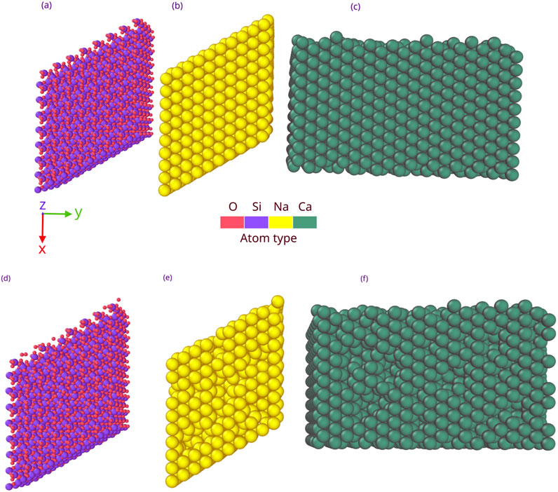
Figure 1. Representations of (a) undamaged SiO₂, (b) undamaged Na, and (c) undamaged Ca slabs. Damaged SiO₂, Na, and Ca slabs are, respectively, represented in (d–f).

The surface of Mercury is under constant irradiation by ions that can create defects in crystals through damage during deposition and sputtering (Navinšek, 1976; Yakshinskiy et al., 2000; Morrissey et al., 2022b). It was shown that such defects could act as stronger binding sites for the volatiles (Morrissey et al., 2022b). This study also explores the effect of damage on the SBE of sulfur for the three different slabs. To simulate damage, atoms were randomly removed from the top atomic layers of the slabs, representing a small amorphous rim of a regolith grain created by radiation (Poppe et al., 2018). Approximately 3% of the total slab was removed from each slab to approximate defects and significantly observe a change in SBE. The slabs were then re-equilibrated in an NVE at 100 K for 50 ps. The three damaged slabs are shown in Figures 1d–f. For each of the six surfaces, a single sulfur atom was deposited from 8 Å above the surface with normal incidence and an energy of 0.15 eV over a randomly selected x–y position. After 30 ps, the deposited atom was either adsorbed or reflected. If the atom was adsorbed, its SBE was evaluated using a method similar to that presented by Morrissey et al. (2021a). This process was repeated 100 times for each substrate to gather statistics.

2.2 Exospheric global model

To simulate the sulfur exosphere of Mercury, we use a 3D EGM that was previously used and validated on multiple solar system objects and for different species (Leblanc and Johnson, 2003; Leblanc and Johnson, 2010; Leblanc et al., 2017; Chaufray et al., 2022; Leblanc et al., 2023a). This 3D EGM was coupled with a subsurface diffusion model, as presented by Verkercke et al. (2024). This coupling allows the surface–exosphere interactions to be studied in-depth as a function of Mercury’s true anomaly angle (TAA).

2.2.1 Exospheric model

The 3D EGM is a time-dependent Monte-Carlo model describing the evolution of individual atoms ejected from Mercury’s surface. The atoms’ motions are influenced by the gravitational fields of Mercury and the Sun, solar radiation pressure, and centrifugal and Coriolis forces (Leblanc and Johnson, 2010). The four ejection processes considered by the model are TD, PSD, SWS, and MMIV. TD is dependent on both the surface temperature and SBE. The probability of ejection through TD, P_TD, is computed as follows (Hodges, 1980; Leblanc and Johnson, 2003; Grava et al., 2021):

$P_{TD}=1-\exp \left(-t_{ad}\right)\text{\hspace{0.17em}with\hspace{0.17em}}{t}_{ad}=t_r{C}^{-1}{T}^2\exp \left(-\frac{U}{k_{b}T}\right),(1)$

where t_r represents the elapsed time as adsorbed, C is a constant including the sulfur vibration frequency taken as 10⁻¹¹sK² (Leblanc and Johnson, 2003; Leblanc and Johnson, 2010; Grava et al., 2021), T represents the surface temperature in K, U represents the SBE, and k_b represents the Boltzmann constant. Regarding PSD, the ejection probability P_PSD can be expressed as Equation 2 (Leblanc and Johnson, 2010; Schmidt, 2013):

$P_{PSD}=1-\exp \left(-t_{PSD}\right)\text{with\hspace{0.17em}}{t}_{\text{PSD}}=t_r\frac{Q_{PSD}{F}_{ph}\cos \left(SZA\right)}{R^2}\exp \left(-\frac{E_A}{k_{b}T}\right),(2)$

where Q_PSD is the photon desorption cross section, F_ph is the photon solar flux at 1 AU, SZA is the solar zenith angle, R is the distance to the Sun in AU, and −E_a is the activation energy in eV. There is no experimental measurement for Q_PSD for S from CaS. Schaible et al. (2020) measured a Q_PSD of 4·10–22 cm² for S photon-stimulated desorption from MgS. Mg and Ca are considered candidates for the formation of sulfur-bearing minerals on Mercury (Bennett et al., 2016; Nittler et al., 2018; Schaible et al., 2020; Renggli et al., 2022; Iacovino et al., 2023; Pommier et al., 2023) because of their divalent cation nature. Bennett et al. (2016) measured a value of 1.1·10–20 cm² for the Ca PSD cross section from CaS. The value obtained from Schaible et al. (2020) is more appropriate as it considers the correct ejected species and is the one used in this work. F_ph was taken as 2.2·1014 photons cm⁻²s⁻¹ (Schmidt, 2013). The EA for S from CaS is also unknown. The EA for Na from SiO₂ was measured by Yakshinskiy and Madey (2004) as being between 0.02 and 0.5 eV. Without any values for S, our study will explore the latter range. The SWS-induced desorption probability P_SWS is considered as Equation 3 (Leblanc and Johnson, 2010):

$P_{SWS}=1-\mathrm{e}\mathrm{x}\mathrm{p}\left({-t}_{SWS}\right)\hspace{0.17em}\text{with}\hspace{0.17em}{t}_{SWS}=t_{r}Y{F}_{SW}{S}_{cell},(3)$

where Y is the yield, F_SW is the solar wind flux at Mercury, and S_cell is the surface of the cell in which the adsorbed atom is contained. Similar to Leblanc and Johnson (2010), Y is taken as equal to 0.06, which is smaller than the value of 0.15 proposed by Killen et al. (2001) to account for the effect of porosity. The solar wind flux is considered to affect only regions of open magnetic field lines, in the same way as described by Leblanc and Johnson (2003) and Leblanc and Johnson (2010).

The last two processes presented above, namely, PSD and SWS, can only influence the desorption of volatiles down to a certain depth before being completely shadowed by the above layers. This depth depends on the porosity of the regolith and the SZA. In order to account for this effect, our study considered a regolith model of the top surface of Mercury, which was simulated using LAMMPS in the same way as described by Verkercke et al. (2023). Ray tracing was applied to the regolith structure at different SZAs to define the maximum depth reached by the rays. As a result, at normal incidence, PSD and SWS are thus considered efficient down to ∼6 mm, while at an SZA close to 90°, the maximum depth reached by these processes is ∼600 µm. Such an approach has already proven necessary to explain observations of variability in other exospheres, such as on Rhea and Dione (Teolis and Waite, 2016), but it has never been applied to Mercury. However, it is clear that the current consideration of a smooth, uniform surface of Mercury is not sufficient to explain all the complexities of the Hermean exosphere surface connection. This method is thus novel compared to those used in previous studies on Mercury.

In the model, the MMIV is considered an injection flux of new atoms rather than a means of ejecting adsorbed particles. It is treated as evolving along Mercury’s orbit and as being non-uniform across Mercury’s surface (Chaufray et al., 2022; Moroni et al., 2023). This injection flux thus depends on the flux of micro-meteoroid impacts and the surface abundances of the species of interest. The former is computed as shown by Chaufray et al. (2022), while the latter originates from the surface abundance maps derived from MESSENGER X-ray spectrometer (XRS) observations (Nittler et al., 2018), which are presented in Figure 2. Above each cell of the surface, the same number of test particles is injected into the exosphere, but their weight W (number of real particles represented by one test particle) varies to account for the meteoroid flux and the surface abundance as Equation 4 (Chaufray et al., 2022):

$W=F_{MM}{n}_{Ca}{S}_{cell}dt,(4)$

where F_MM is the flux of micro-meteoroid impacts that varies according to the position on the planet’s surface and the TAA, n_Ca is the surface abundance of S observed by MESSENGER XRS, which also varies with the geographical position (cf. Figure 2), and dt is the period ejection in the simulation.

Figure 2

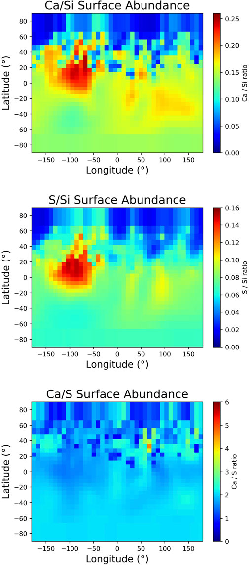
Figure 2. Relative surface abundance maps of (top) S/Si, (middle) Ca/Si, and (bottom) Ca/S derived from MESSENGER XRS observations and degraded to the EGM grid resolution. The latitudes and longitudes are, respectively, northern and eastern.

In addition to this MMIV source, another uniform source is considered and described in Section 2.2.2. As the abundance maps from XRS are relative, our study uses a total surface density of volatiles of 7.5·10¹⁴ cm⁻² (Killen et al., 2001).

Once ejected, an atom can be ionized and is considered lost by the simulation. It can also re-impact the surface and either reflect or adsorb. Upon reflection, the model considers perfect accommodation of the reflected atoms with their energy proportional to the local surface temperature. The adsorption probability of a sulfur atom re-impacting the surface is considered the probability of this atom falling onto a calcium-bearing surface (see Section 3.1). S adsorption is thus directly computed using the Ca map shown in Figure 2. Once adsorbed on the surface, an atom can either get re-ejected into the exosphere or diffuse into the subsurface of Mercury. This latter possibility is presented below.

2.2.2 Surface and subsurface parametrization

Previous exosphere models only considered the surface as impermeable to gas (Wurz and Lammer, 2003; Leblanc and Johnson, 2010) or treated the gas diffusion as a simple injection term that did not depend on the exosphere feedback on the surface (Mura et al., 2023). Our work considers a subsurface that is directly coupled with the exosphere, where the exospheric particles are tracked even when returning to the regolith. This allows following the global evolution of sulfur content in Mercury’s environment while studying the coupling between the exosphere and the surface, based only on physical processes and without any ad-hoc constrains. To the best of our knowledge, this is the first time such an approach has been considered for the study of the Hermean exosphere. Moreover, no 3D exosphere simulation has ever been attempted to describe sulfur variability at Mercury.

In our model, the subsurface is described as 50 layers extending from the surface down to 1 m depth. The top surface layer has a thickness of 50 μm, which is close to the mean size of a regolith grain (McKay et al., 1991; Wurz et al., 2010). The layer size increases downward, with the last layer having a thickness of 5 cm. The temperature evolution of the regolith is described using the heat equation as follows:

$\rho C_p\frac{\partial T}{\partial t}=\frac{\partial }{\partial z}\left(k\frac{\partial T}{\partial z}\right),(5)$

where ρ is the density, k is the thermal conductivity, and C_p is the specific heat, all varying with the depth z and the temperature T. These parameters are taken from Verkercke et al. (2024). The regolith is assumed to be in thermodynamic equilibrium. The top and bottom boundary conditions are, respectively, ruled by the solar and infrared radiations and the geothermal heat flux (Yan et al., 2006). At the surface, Equation 5 takes the following forms on the day and night sides:

$\rho C_p\frac{\partial T_s}{\partial t}=\frac{\partial }{\partial z}\left(k\frac{\partial T}{\partial z}\right){|}_s+\frac{\sigma \epsilon }{d_s}\left(T_{sky}^4-T_s^4\right)+D_s\frac{1-A}{d_s}\frac{F_S}{R2}\cos \left(SZA\right)(6)$

and

$\rho C_p\frac{\partial T_s}{\partial t}=\frac{\partial }{\partial z}\left(k\frac{\partial T}{\partial z}\right){|}_s+\frac{\sigma \epsilon }{d_s}\left(T_{sky}^4-T_s^4\right).(7)$

The three terms on the right-hand side of Equation 6 are, from left to right, the heat conduction flux, the radiated energy flux, and the solar flux received by the top of the regolith, respectively. Here, d_s is the surface layer thickness of 50 μm, σ is the Stefan–Boltzmann constant, ϵ = 0.9 is the emissivity (Chase et al., 1976), T_s and T_sky are, respectively, the surface and sky temperatures, with T_sky = 3 K (Yan et al., 2006), A is the Bond albedo, with A = 0.12 (Veverka et al., 1988), F_S is the solar constant equal to 1,367 W m^–2, and R is the heliocentric distance in AU. In Mercury’s sky, the solar disk has an apparent size of ∼1.5°, which influences the temperatures at the terminators and poles. In our model, it is represented by the factor D_s, the apparent fraction of the solar disk (Salvail and Fanale, 1994). The last term of Equation 6 is null on the night side, resulting in Equation 7. At the bottom boundary, the heat equation can be expressed as Equation 8:

$\rho C_p\frac{\partial T_b}{\partial t}=\frac{\partial }{\partial z}\left(k\frac{\partial T}{\partial z}\right){|}_b+\frac{J_b}{d_b},(8)$

where the geothermal heat flux J_b = 2·10^–2 W m^–2 (Yan et al., 2006) and d_b is the deepest layer’s thickness.

In order to constrain the surface abundances of the species and, thus, the adsorption probability, one can use MESSENGER XRS observations of the chemical composition of Mercury’s regolith. The Ca/Si, S/Si, and Ca/S surface abundance maps derived from MESSENGER XRS observations and degraded to match the EGM surface grid are presented in Figure 2. Here, we assume that sulfur only deposits on Ca-bearing regions as MESSENGER XRS observations showed a nearly uniform 2:1 Ca/S surface abundance ratio all over Mercury (Nittler et al., 2018; Nittler et al., 2020) (Figure 2). This approximation is also supported by laboratory measurements (Renggli et al., 2022) described in Section 3.1. We consider that the abundances derived from MESSENGER XRS measurements are similar at 1 m of depth than at the surface. However, the uniform source represents a constant contribution to the ejection processes from freshly exposed grains and is considered to be uniform across the planet’s entire surface. It is constrained to the top 6 mm of the regolith, where the ejection processes are efficient, and is arbitrarily fixed at 10⁶ S/cm²/s, but since our study focuses on general variability rather than on determining specific densities, this will not affect our results. As an atom impacts the surface, it can potentially reach deeper regions in the regolith before it first encounters a grain due to the surface porosity, similar to the PSD and SWS ejection processes. However, these do not depend on the SZA but solely on the regolith structure. Sulfur atoms impacting the surface are thus considered to be randomly distributed in the first 6 mm of regolith. Once adsorbed, the atom can diffuse vertically in the regolith (Teolis and Waite, 2016; Reiss et al., 2021; Teolis et al., 2023; Verkercke et al., 2024). The model only considers Knudsen diffusion, which happens through repeated adsorption/desorption or collisions with the regolith grains. This diffusion is thus highly dependent on both the regolith temperature and the SBE of the volatile with the regolith (Verkercke et al., 2024). Volatiles can get trapped in the regolith, causing a lag in their ejection and highlighting the need to consider more than just single-layer surfaces in exospheric models (Sarantos and Tsavachidis, 2021).

3 Predicted variability in sulfur on Mercury

3.1 Evaluation of surface binding energies

Our MD simulation of S deposition on the SiO₂ samples showed that none of the deposited sulfur atoms bonded with the surface, yielding a 100% reflection rate. This result agrees well with experiments by Renggli et al. (2022), who deposited sulfur on Mercury analog materials and found anti-correlation between the presence of Si and S in their samples. This is coherent with the fact that in an environment as highly reduced as Mercury’s surface, S is mostly in a S²⁻ form, leading to repulsion between O (contained in silicates) and S (Pommier et al., 2023). At low oxygen fugacity, S can form SiS₂ only at high temperature and pressure (Iacovino et al., 2023; Pommier et al., 2023). The high temperatures and pressures needed for such formation are not reproduced on Mercury without impacts (Iacovino et al., 2023; Pommier et al., 2023).

For the Na and Ca samples, the computed SBE distributions are given, respectively, in Figures 3a, b. In the case of the perfect crystals, the SBEs are very low, with mean values of 0.13 and 0.53 eV and standard deviations of 0.016 and 0.024 eV, respectively, for Na and Ca. The mean SBE value for S on Na is quite similar to the value of 0.27 eV of Na in sulfur-bearing molecules proposed by Wiens et al. (1997). It is interesting to note that S forms stronger bonds on Ca than on Na, which again is coherent with the results of Renggli et al. (2022), which showed a correlation between Ca- and S-rich regions, while Na- and S-rich regions were almost never correlated. The values do not vary significantly as S atoms have very little diversity in the binding sites due to the repeated coordination within the perfect crystal structure. The greater SBEs found for S on Ca are further supported by the higher enthalpy of CaS than that of Na₂S (Haynes, 2014).

Figure 3

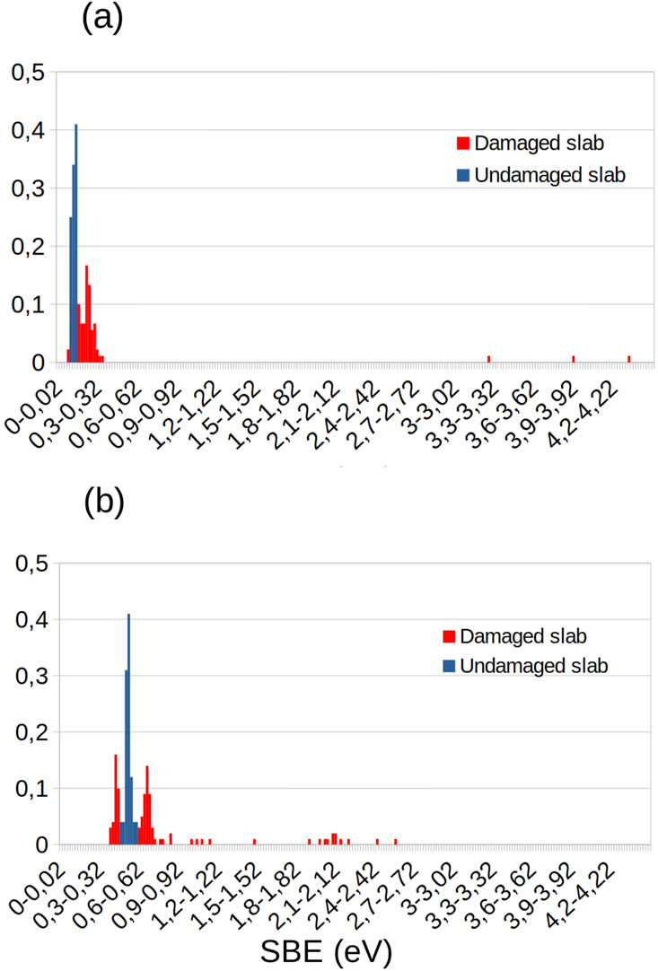
Figure 3. SBE distributions of S on (a) a Na crystal and (b) a Ca crystal. The blue (orange) distribution represents the SBE for S atoms on undamaged (damaged) crystals.

When including defects, this diversity expands, as shown in orange by the larger SBE distributions shown in Figures 3a, b. One can also observe that S atoms are efficiently trapped in defects, where they have much higher SBE values than on perfect crystals. The maximum value of SBE is larger on a damaged Na slab (4.3 eV) than on a damaged Ca slab (2.6 eV). This might be caused by the lower metallic binding between Na atoms, which allows them to vibrate around and cover an adsorbed S atom, while Ca atoms have stronger metallic bonds due to their higher valence (Saleh, 2021). This could also happen for Ca at higher temperatures. However, as shown in Figure 3, the probability of efficient trapping (SBE > 1.5 eV) in a defect is higher on a damaged Ca slab. For both undamaged Na and Ca crystals, the reflection rates are null, meaning that any S atom falling on the surface is adsorbed. However, once damages are introduced, the reflection rate increases to ∼3% on a Na surface, while it stays null on Ca. This can be explained by the more diverse types of sites on which an S atom can fall, leading to a broader SBE distribution. As SBE values on an undamaged Na slab are already small, even weaker SBE values arise due to the presence of damages, which creates the possibility of reflection. We also considered the case of S deposited onto an SiO₂ crystal nearly totally covered with a layer of Ca atoms. Such deposition showed a 100% reflection rate, similar to the pure SiO₂ surface, which is again coherent with the results of Renggli et al. (2022), showing that regions containing both Ca and Si are free of sulfur. This could be attributed to the long-range repulsion of S and O in such a reduced environment, which would need several Ca layers to shield S from underlying O and result in adsorption. Based on these results and as S seems to adsorb preferentially on Ca rather than on Na or SiO₂, our study will approximate that S only deposits on damaged Ca crystal structures while only considering the higher SBE (1.9–2.6 eV) caused by the defects. These SBE values are coherent with the values used by Wurz and Lammer (2003) in their model. However, the latter model only considered a single SBE value, whereas our work includes a more detailed description of the gas–surface interaction. Considering only the higher values avoids computing repetitive small bounces and allows the model to focus on long-term adsorption. Weakly bound deposited atoms can diffuse along the surface until they cross a defect, which would sample the SBEs we focus on in this study (Yakshinskiy et al., 2000; Morrissey et al., 2022b).

3.2 Hermean sulfur exosphere

This work focuses on the variability of the densities predicted by an MD-informed EGM capturing both the exosphere and Mercury’s subsurface. While results are described as densities or column densities, these depend strongly on the amount of sulfur used as input for our exospheric calculations, a quantity that is poorly constrained. As a consequence, this work aims to provide a description of the variability of its structure and not of the exact total amount of sulfur in the exosphere and subsurface.

The present simulation uses the Q_PSD value presented by Schaible et al. (2020) and an activation energy E_A = 0.4 eV (Yakshinskiy and Madey, 2004). To include the MD results presented in Section 3.1, each test particle is introduced in the simulation with an SBE that is randomly selected out of the highest part of the orange distribution of SBE (1.9–2.6 eV) (cf. Figure 3B), representing S trapped in Ca crystal defects. Figure 4 shows a diagram summarizing how the different models (EGM, thermal model, and diffusion model) are coupled in this MD-informed EGM.

Figure 4

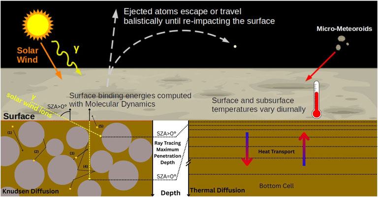
Figure 4. Diagram of the coupling of the three different models (EGM, Knudsen diffusion, and thermal). Above the surface, EGM describes the exospheric transport and the injection of particles through micro-meteoroid impacts. As an atom returns to the surface, it can fall in the regolith subsurface and diffuse, following the Knudsen diffusion diagram (bottom left). (1) The atom enters the regolith depths. (2) A newly injected atom or a previously adsorbed atom desorbs and re-adsorbs on another grain, where a new SBE value is attributed. (3) Same as (2) but the atom keeps diffusing toward the surface. Desorption can be caused by the processes described in Section 2.2.1, some of which depend on the SZA and the depth (computed with ray tracing in yellow). (4) An atom desorbs and diffuses deeper than the maximum depth reached by the photons and solar ions. This atom diffusion is now purely thermal, with the regolith temperature as a function of depth described by the model sketched in the bottom right. An atom diffusing too deeply in the regolith can result in a permanent sink, depending on the regolith temperature and the SBE (as shown by Equation 1). (5) The atom escapes the regolith and enters the exosphere.

The simulation is initialized at aphelion and runs for two Mercury years to ensure that the results do not depend on the initial conditions. The simulation outputs are based on the two following years, making a total of 4 Mercury years of simulation. Using two different spatial scales and two different color bars, Figure 5 presents the exospheric and subsurface density map in the equatorial plane at different orbital positions in the Mercury solar orbital (MSO) coordinate system. The origin is centered at Mercury’s center of mass, the x-axis points sunward, the y-axis points at dusk, and the z-axis points northward. The exospheric map extends spatially from the surface to 2,000 km in altitude, while the subsurface map extends from the surface down to 0.75 m of depth following the scale plotted in the center of each map of Figure 5. The model predicts a sulfur exosphere that is globally populated by thermal and micro-meteoroid impact-induced ejections at any orbital position. Due to the 3:2 spin-orbit resonance of Mercury and its eccentric orbit, the longitudes at local noon at perihelion (TAA 0°) are more exposed to the Sun than all other longitudes, forming “hot poles” (Soter and Ulrichs, 1967; Leblanc et al., 2023b). The hot poles are indicated as green dashed lines in Figure 5.

Figure 5

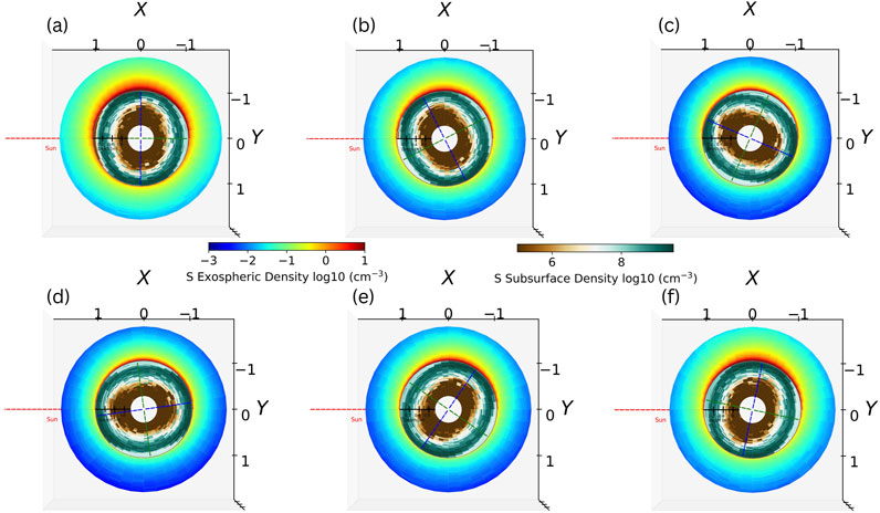
Figure 5. Exospheric and subsurface density maps in the equatorial plane at different orbital positions using the Mercury solar orbital (MSO) coordinate system. The red dashed line indicates the Sun’s direction. The blue and green dashed lines indicate the cold and hot longitudes, respectively. The spatial scale of the exosphere is expressed in planetary radii and is indicated on the axis of the figures, while the subsurface scale is indicated in meter at the center of each map. (a) TAA = 010°. (b) TAA = 120°. (c) TAA = 160°. (d) TAA = 186°. (e) TAA = 230°. (f) TAA = 265°.

3.2.1 Perihelion

Figure 5a shows that close to perihelion, when the surface temperature reaches its maximum, the sulfur exosphere is the densest at dawn. The higher surface temperatures around the hot poles also deplete the top of the Hermean regolith of its sulfur content. As the heat waves propagate deeper at these longitudes, the diffusion of sulfur is efficient deeper in the regolith, forming a reservoir below 10 cm of depth with a density peak of approximately 21 cm. At this orbital position, the longitudes facing dawn and dusk at perihelion are the least exposed to the Sun, forming “cold poles” (Soter and Ulrichs, 1967). The cold poles are indicated as blue dashed lines in Figure 5. These colder temperatures limit the thermal desorption of atoms in the exosphere and the diffusion depth of the volatiles, forming shallower sulfur reservoirs at these positions, which peak at approximately 8 cm of depth. On average, the overall content of sulfur on the surface is approximately 6.7 times greater at the cold longitudes than at the hot longitudes. The sulfur exosphere exhibits a dawn–dusk asymmetry due to the micro-meteoroid flux, which is the highest around perihelion and is the maximum at 6 local time (LT) in our simulation (Chaufray et al., 2022). This induces the exospheric peak density to be located at 6 LT. Thermal desorption and photon-stimulated desorption contribute to the sulfur release on the day side as secondary processes as most of the sulfur has either been released or has diffused deep in the regolith, from where it cannot escape.

3.2.2 Outbound leg, aphelion, and inbound leg

As Mercury moves outbound, its sulfur exosphere scale height and density decrease as the surface temperature also starts to decrease. Moreover, the micro-meteoroid flux reduces during the outbound leg, lowering the density at dawn. Simultaneously, the cold longitude that was previously at dawn is closer to local noon as the planet gets closer to aphelion (TAA 180°) (Figures 5b, c). As the hot pole rotates in the afternoon, its surface temperature decreases, while the heat wave propagates deeper in the regolith. These combined influences decrease the efficiency of the ejection processes while allowing some subsurface atoms to diffuse upward into the surface, resulting in a replenishment of the sulfur content in the top few centimeters of the regolith (Figures 5a–c). Figure 6 represents the mean sulfur exospheric density 2 km above the surface at the equator as a function of MSO longitudes during aphelion and the inbound leg. The red and blue solid vertical lines represent the cold longitudes at −90°E and 90°E (cf. Figure 2), respectively. The region around each cold pole is depicted by dashed lines of the same color and is defined as the region extending 45° west and east to the cold longitude. Figures 6a–c show that the 90°E cold longitude exhibits a local increase in the exospheric density above the cold pole (blue) as it reaches the sub-solar point when its enriched surface caused by its lower temperature heats up and releases S atoms in the exosphere. One can also notice that simultaneously, as the other cold pole evolves toward dawn, its higher S surface abundance increases the micro-meteoroid-impact release of S on the night side, forming an asymmetry in the exosphere around dawn. Figure 2 shows that the cold pole around −90°E presents a higher Ca abundance, leading to a higher adsorption probability of S. Figures 6d–f show that this increased Ca abundance also enriches the surface in sulfur and that passage at the sub-solar point causes a larger release of sulfur in the exosphere with respect to the other cold pole. Conversely, the exospheric density at the dawn terminator is smaller when the 90°E cold longitude rotates toward this position as its sulfur content is smaller, reducing the micro-meteoroid ejection rate. This suggests that the sulfur exosphere exhibits a period of 2 years, similar to the Mg exosphere (Chaufray et al., 2022), rather than the 1-year period as observed for the sodium exosphere (Cassidy et al., 2015; Cassidy et al., 2016). As the cold longitudes rotate away from the sub-solar point, the cold poles’ exospheric enhancement fades as the efficiencies of the ejection processes decrease. However, the enhancement remains present in the local afternoon. Such cold pole enhancement of exospheric volatiles has been observed by MESSENGER in Mercury’s sodium exosphere (Cassidy et al., 2016; Mura et al., 2023). In the inbound leg after TAA 200°, the sulfur exospheric density increases globally until Mercury reaches perihelion (Figures 5d–f). Moving inbound, the micro-meteoroid flux increases as well, which increases the density at dawn. Figure 6 exhibits this increase as the cold poles return to the terminators.

Figure 6

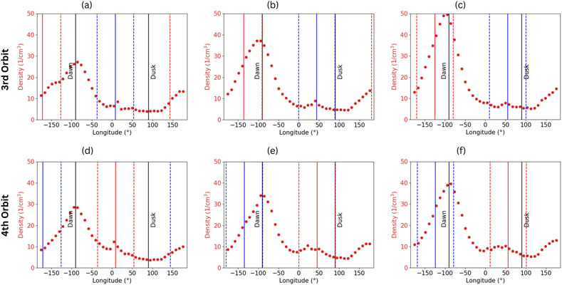
Figure 6. Exospheric density 2 km above the surface at the equator as a function of the MSO longitude and focused after aphelion, showing the cold longitude passage from noon to dusk. The first and second row, respectively, present the third and fourth orbit simulated in EGM. The third orbit shows the passage of the 90°E cold longitude, whereas the fourth shows the −90°E cold longitude passage. (a) TAA = 186°. (b) TAA = 218°. (c) TAA = 230°. (d) TAA = 187°. (e) TAA = 219°. (f) TAA = 231°.

During the whole orbit, Mercury’s exosphere is denser on the night side than on the day side, up to a factor of 4 close to the surface, due to an overall migration of the atoms toward the night side. Since the adsorption probability is considered proportional to the Ca abundance, which is lower than 1 (cf. Section 2), an exospheric atom can hop many times on the surface before being adsorbed. As a reflected atom is considered to fully accommodate with the surface, an atom is less energetic when it reflects on the night side, making its next successive “hops” closer to one another than if the same atom had fallen on the hotter day-side surface. As Ca abundance is the smallest at high northward latitudes, S atoms tend to remain longer in the exosphere above such regions, forming a local enhancement and a north–south asymmetry on the night side. Moreover, the day side is subject to photo-ionization, which is considered a loss term in our model, reducing the amount of S in the day-side exosphere. As the lifetime of sulfur against photo-ionization is ∼6·10⁵ s (Huebner and Mukherjee, 2015), this can significantly affect the day-side exosphere. Finally, the hotter surface also allows atoms to diffuse in the surface, which constitutes another loss term for the day-side exosphere.

3.3 Calcium influence on sulfur

Our model assumes that S can only bond with Ca and constrains this using the abundance map of Ca presented in Figure 2. In order to investigate the influence of calcium surface abundance on the sulfur exosphere, one can study the sulfur reservoir formed in the Hermean regolith. This accumulation depends on Ca abundance and solar exposure, which influence the surface temperature; in turn, the temperature controls subsurface diffusion and the ejection processes (Leblanc and Johnson, 2010). One could thus expect the Hermean regolith to be depleted of S at the hot poles and enriched at the cold poles. Figure 2 presents a strong enhancement of Ca abundance (−90°E) with respect to the other cold longitude. Such a difference is expected to influence the accumulation of S in Mercury’s regolith. Figure 7 presents the synodic average of the sulfur column density in the Herman regolith down to 0.75 m. The iso-contours show the Ca abundance map from Figure 2. It is clear that the hot poles appear depleted with respect to the cold poles and do not exhibit any correlation with Ca abundance. The regions at latitudes between 40° and 60° in both hemispheres are also depleted due to an efficient sputtering release. However, both cold poles efficiently retain sulfur, especially eastward to the cold longitudes. This can be attributed to the depletion of S at the hot poles, where sulfur was preferentially ejected, allowing it to migrate to the terminators, where the surface temperatures are colder. At dawn, the atoms that have adsorbed on the surface will later be rotated to the day side, where they can desorb again. This cycle continues until the atoms reach regions that allow longer residency time, such as the cold poles or deeper reservoirs.

Figure 7

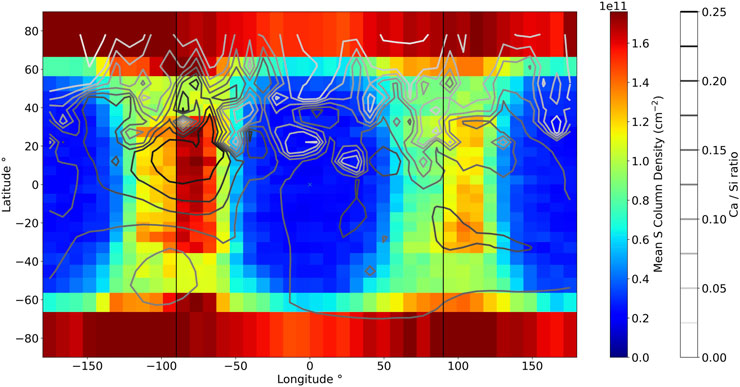
Figure 7. Map of the mean sulfur column density in the regolith from EGM over one synodic cycle. The contour shows the Ca abundance map derived by MESSENGER XRS presented in Figure A.

Additionally, the cold pole exhibiting the enhancement of Ca at the surface also exhibits a globally larger mean S column density in the regolith than the other cold pole. This induces a sulfur content that is ∼1.4 times greater at the −90°E cold longitude than at the 90°E cold longitude. It would also appear that both cold poles exhibit north–south asymmetries. The cold pole at −90°E exhibits a larger S content around Ca enhancement than southward to it. The southward region of this cold pole, however, exhibits a larger content of sulfur than what is expected from its Ca content. This enhancement can be explained by ejected sulfur from the northward Ca-rich region, which migrates southward and gets adsorbed in this region. This influence is confirmed as the same simulation was performed with a uniform Ca surface abundance and does not exhibit any difference between the cold longitudes. The cold pole at 90°E presents a slight enhancement of Ca south to the equator that matches the higher sulfur content in this region with respect to the region northward at the same longitudes. This suggests that Ca abundance can influence where S is preferentially adsorbed when the thermal conditions allow for adsorption. One could point out that the North and South poles are predicted to be very enriched in sulfur. Sulfur reaching these poles interacts with a surface that is cold compared to the rest of the planet as it is barely exposed to the Sun. Atoms adsorbing at these regions cannot diffuse downward or desorb due to the lack of an efficient desorption process, trapping them at the top surface of the regolith. A sulfur enhancement of the poles has also already been suggested to explain high albedo regions observed at Mercury’s poles (Sprague et al., 1995). MESSENGER XRS did not detect such pole enhancement, which could be due to the lack of solar flare X-rays reaching these regions or due to difficulty in observing these regions (Nittler et al., 2020).

4 Conclusion

Using a 3D exospheric global model, this study predicts the variability in the neutral sulfur exosphere at Mercury. We constrain the sulfur ejection of Mercury’s surface by computing the SBE distribution of S on different crystalline substrates in different states using MD. Although no adsorption of S was observed for the SiO₂ substrate, sulfur can deposit on pure Na and pure Ca substrates. The inability of S to deposit on SiO₂ is attributed to the similar charge that S and O present in a highly reduced environment, such as Mercury, leading to repulsion between the two species (Iacovino et al., 2023; Pommier et al., 2023). Additionally, laboratory experiments of S deposition on Mercury analog materials, conducted by Renggli et al. (2022), showed an anti-correlation between the presence of S and the presence of Si in the sample, leading to a similar conclusion. For perfect crystals of Na and Ca, S exhibits higher SBE values on the latter than on the former. By including defects in the crystal lattices, the SBE increased for both Na and Ca, but the values are globally higher for Ca, with a probability greater than 0.1 to have a value above 1.9 eV. This is consistent with the findings of Renggli et al. (2022), who observed a strong correlation between the deposition of S and the presence of Ca in Mercury analog materials. A similar correlation was observed in MESSENGER XRS measurements of Ca and S surface abundances at Mercury, which also exhibit a strong correlation (Nittler et al., 2018). These results show that sulfur can bond particularly strongly with calcium, which induces a correlation between the surface abundances of both species. However, this study mostly considered the adsorption of S at 100 K, whereas the SBE can change as a function of the substrate temperatures and coverage (Yakshinskiy and Madey, 2004). Future work should consider a dynamic evolution of this parameter.

With the surface adsorption of S constrained by calcium abundance measured by MESSENGER XRS and using a photon cross section proposed by Schaible et al. (2020), we predict that the sulfur exosphere is mostly ejected by micro-meteoroid impacts, with a non-negligible thermal population due to the perfect accommodation with the surface. The S exosphere is predicted to be the densest at perihelion, with an exospheric density peak at dawn due to a contribution of micro-meteoroids, a thermal ejection efficiency that is higher at this orbital position, and the enhancement of volatiles at the surface close to the terminators because they accumulate there due to the lower surface temperatures (Cassidy et al., 2015). The ejection processes are all more efficient when Mercury is closest to the Sun. At the same time, the longitudes facing the Sun (close to local noon) reach high temperatures that favor deeper Knudsen diffusion (Teolis et al., 2023; Verkercke et al., 2024). This causes a rapid depletion of S at these hot longitude surfaces while forming deeper reservoirs—approximately 20 cm deep. Moving outbound toward aphelion, the sulfur exospheric density decreases globally. This can be attributed to the lower ejection efficiencies at aphelion than at perihelion. These colder surface temperatures favor the retention of volatiles and significantly reduce S diffusion depth, leading to a peak surface density of sulfur at the cold poles and the formation of a subsurface reservoir at a shallower depth—approximately 8 cm deep. These cold longitudes are thus expected to present higher S abundance close to the surface of Mercury. This surface enhancement is predicted to have a local influence on the exosphere, inducing a density enhancement over these cold poles. Such enhancement occurs as soon as the cold poles rotate from dawn to noon, reaching a peak around noon before decreasing during the afternoon. Such behavior seems plausible as it was also detected by MESSENGER in Mercury’s Na exosphere (Cassidy et al., 2016). The cold pole surfaces westward to the hot poles are enhanced in S due to the high release rate of the hot poles and the preferential migration of the atoms toward the terminators due to lower temperatures.

Additionally, Ca surface abundance influences the S retention over the cold poles, favoring the adsorption of S where the surface is richer in Ca. This causes a significant difference between the S contents of the two cold longitudes and north–south asymmetries. The Ca-rich region at −90°E causes this cold pole to accumulate ∼1.4 times more sulfur than the other cold longitude, which creates a larger exospheric enhancement when it reaches the day side. The sulfur exosphere also exhibits a day–night asymmetry, with a globally higher density over the night side. This is due to the migration of atoms toward the night side, which fully accommodates the cold surface temperatures, lowering the energy of the reflected atoms. A northern exospheric enhancement is predicted due to its low Ca surface abundance, which decreases the adsorption probability locally. A sulfur enhancement of the North and South poles is predicted by Sprague et al. (1995) but is unseen by MESSENGER XRS. This discrepancy could be due to the elliptic polar orbit of MESSENGER, which did not allow for high spatial resolution at the South Pole and provided limited coverage of the North Pole. Additionally, solar flares were needed to observe the relative abundance of sulfur, which did not occur continuously (Nittler et al., 2020).

Our study concludes that the sulfur exosphere variability at Mercury depends mostly on the micro-meteoroid flux. The surface and subsurface content of sulfur are, however, mostly dictated by the thermal and chemical properties of the regolith, depleting the sulfur density at the hot poles and enhancing it at the cold poles, particularly where Ca is present. Our model predicts that the best time to perform measurements would be around perihelion close to dawn, where the simulated S exosphere exhibits the largest density. Our modeling shows that volatiles could accumulate in the subsurface, in agreement with the inferred subsurface enhancement of sulfur (Barraud et al., 2023), which could be linked to surface geomorphic features such as hollows. These results can be tested by observations to be made by the upcoming BepiColombo mission.

Data availability statement

The raw data supporting the conclusions of this article will be made available by the authors, without undue reservation.

Author contributions

SV: Conceptualization, Formal analysis, Investigation, Methodology, Software, Validation, Visualization, Writing – original draft, Writing – review and editing. JYC: Conceptualization, Methodology, Software, Supervision, Validation, Writing – review and editing. FL: Conceptualization, Methodology, Software, Supervision, Validation, Writing – review and editing. AG: Software, Validation, Writing – review and editing. MP: Conceptualization, Methodology, Supervision, Writing – review and editing. GM: Conceptualization, Methodology, Supervision, Writing – review and editing. JL: Software, Writing – review and editing. AR: Software, Writing – review and editing. LM: Conceptualization, Methodology, Software, Supervision, Writing – review and editing.

Funding

The author(s) declare that financial support was received for the research and/or publication of this article. SV, FL, and JYC acknowledge the support of ANR, France, of the TEMPETE project (grant No. ANR-17-CE31-0016) and the support of CNES, France, for the BepiColombo mission. This research was supported by the International Space Science Institute (ISSI) in Bern through the ISSI International Team project #559 “Improving the Description of Exosphere Surface Interface” and the ISSI International Team project #616 “Multi-scale Understanding of Surface-Exosphere Connections (MUSEC).” The authors also acknowledge the support of the IPSL CICLAD data center for providing access to their computing resources and data.

Conflict of interest

The authors declare that the research was conducted in the absence of any commercial or financial relationships that could be construed as a potential conflict of interest.

The handling editor SK declared a shared affiliation with the author JVC at the time of review.

Generative AI statement

The author(s) declare that no Generative AI was used in the creation of this manuscript.

Publisher’s note

All claims expressed in this article are solely those of the authors and do not necessarily represent those of their affiliated organizations, or those of the publisher, the editors and the reviewers. Any product that may be evaluated in this article, or claim that may be made by its manufacturer, is not guaranteed or endorsed by the publisher.

References

Aktulga, H. M., Fogarty, J. C., Pandit, S. A., and Grama, A. Y. (2012). Parallel reactive molecular dynamics: numerical methods and algorithmic techniques. parallel Comput. 38 (4-5), 245–259. doi:10.1016/j.parco.2011.08.005

CrossRef Full Text | Google Scholar

Barraud, O., Besse, S., and Doressoundiram, A. (2023). Low sulfide concentration in Mercury’s smooth plains inhibits hollows. Sci. Adv. 9 (12), eadd6452. doi:10.1126/sciadv.add6452

PubMed Abstract | CrossRef Full Text | Google Scholar

Baudin, M., Wójcik, M., and Hermansson, K. (1997). A molecular dynamics study of MgO (111) slabs. Surf. Sci. 375 (Issues 2–3), 374–384. doi:10.1016/S0039-6028(96)01289-7

CrossRef Full Text | Google Scholar

Bennett, C. J., McLain, J. L., Sarantos, M., Gann, R. D., DeSimone, A., and Orlando, T. M. (2016). Investigating potential sources of Mercury's exospheric Calcium: photon-stimulated desorption of Calcium Sulfide. J. Geophys. Res. Planets 121 (2), 137–146. doi:10.1002/2015je004966

CrossRef Full Text | Google Scholar

Blewett, D. T., Stadermann, A. C., Susorney, H. C., Ernst, C. M., Xiao, Z., Chabot, N. L., et al. (2016). Analysis of MESSENGER high-resolution images of Mercury’s hollows and implications for hollow formation. J. Geophys. Res. Planets 121 (9), 1798–1813. doi:10.1002/2016JE005070

CrossRef Full Text | Google Scholar

Broadfoot, A. L., Shemansky, D. E., and Kumar, S. (1976). Mariner 10: mercury atmosphere. Geophys. Res. Lett. 3, 577–580. doi:10.1029/GL003i010p00577

CrossRef Full Text | Google Scholar

Cassidy, T. A., McClintock, W. E., Killen, R. M., Sarantos, M., Merkel, A. W., Vervack Jr, R. J., et al. (2016). A cold-pole enhancement in Mercury’s sodium exosphere. Geophys. Res. Lett. 43 (21), 12111–11128. doi:10.1002/2016GL071071

PubMed Abstract | CrossRef Full Text | Google Scholar

Cassidy, T. A., Merkel, A. W., Burger, M. H., Sarantos, M., Killen, R. M., McClintock, W. E., et al. (2015). Mercury’s seasonal sodium exosphere: MESSENGER orbital observations. Icarus 248, 547–559. doi:10.1016/j.icarus.2014.10.037

CrossRef Full Text | Google Scholar

Chase, S. C., Miner, E. D., Morrison, D., Münch, G., and Neugebauer, G. (1976). Mariner 10 infrared radiometer results: temperatures and thermal properties of the surface of Mercury. Icarus 28 (4), 565–578. doi:10.1016/0019-1035(76)90130-5

CrossRef Full Text | Google Scholar

Chaufray, J. Y., Leblanc, F., Werner, A. I. E., Modolo, R., and Aizawa, S. (2022). Seasonal variations of Mg and Ca in the exosphere of Mercury. Icarus 384, 115081. doi:10.1016/j.icarus.2022.115081

CrossRef Full Text | Google Scholar

Grava, C., Killen, R. M., Benna, M., Berezhnoy, A. A., Halekas, J. S., Leblanc, F., et al. (2021). Volatiles and refractories in surface-bounded exospheres in the inner solar System. Space Sci. Rev. 217 (2021), 61. doi:10.1007/s11214-021-00833-8

PubMed Abstract | CrossRef Full Text | Google Scholar

Haynes, W. M. (2014). CRC handbook of chemistry and physics. Boca Raton: CRC Press.

Google Scholar

Hodges, R. R. (1980). “Lunar cold traps and their influence on argon-40,” in Lunar and planetary science conference, 11th proceedings. Houston, TX, 17-21 March, 1980 (Pergamon Press), 2463–2477.

Google Scholar

Huebner, W. F., and Mukherjee, J. (2015). Photoionization and photodissociation rates in solar and blackbody radiation fields. Planet. Space Sci. 106, 11–45. doi:10.1016/j.pss.2014.11.022

CrossRef Full Text | Google Scholar

Iacovino, K., McCubbin, F. M., Vander Kaaden, K. E., Clark, J., Wittmann, A., Jakubek, R. S., et al. (2023). Carbon as a key driver of super-reduced explosive volcanism on Mercury: evidence from graphite-melt smelting experiments. Earth Planet. Sci. Lett. 602, 117908. doi:10.1016/j.epsl.2022.117908

CrossRef Full Text | Google Scholar

Killen, R. M., Cremonese, G., Lammer, H., Orsini, S., Potter, A. E., Sprague, A. L., et al. (2007). Processes that promote and deplete the exosphere of mercury. Space Sci. Rev. 132, 433–509. doi:10.1007/s11214-007-9232-0

CrossRef Full Text | Google Scholar

Killen, R. M., and Morgan, T. H. (1993). Diffusion of Na and K in the uppermost regolith of Mercury. J. Geophys. Res. Planets 98 (E12), 23589–23601. doi:10.1029/93JE02617

CrossRef Full Text | Google Scholar

Killen, R. M., Morrissey, L. S., Burger, M. H., Vervack, R. J., Tucker, O. J., and Savin, D. W. (2022). The influence of surface binding energy on sputtering in models of the sodium exosphere of Mercury. Planet. Sci. J. 3 (6), 139. doi:10.3847/PSJ/ac67de

CrossRef Full Text | Google Scholar

Killen, R. M., Potter, A. E., Reiff, P., Sarantos, M., Jackson, B. V., Hick, P., et al. (2001). Evidence for space weather at Mercury. J. Geophys. Res. Planets 106 (E9), 20509–20525. doi:10.1029/2000je001401

CrossRef Full Text | Google Scholar

Killen, R. M. D. E., Shemansky, D., and Mouawad, N. (2009). Expected emission from Mercury's exospheric species, and their ultraviolet–visible signatures. Astrophysical J. Suppl. Ser. 181 (2), 351–359. doi:10.1088/0067-0049/181/2/351

CrossRef Full Text | Google Scholar

Lark, L. H., Head, J. W., and Huber, C. (2023). Evidence for a carbon-rich Mercury from the distribution of low-reflectance material (LRM) associated with large impact basins. Earth Planet. Sci. Lett. 613, 118192. doi:10.1016/j.epsl.2023.118192

CrossRef Full Text | Google Scholar

Leblanc, F., and Johnson, R. E. (2003). Mercury’s sodium exosphere. Icarus 164 (2), 261–281. doi:10.1016/S0019-1035(03)00147-7

CrossRef Full Text | Google Scholar

Leblanc, F., and Johnson, R. E. (2010). Mercury exosphere I. Global circulation model of its sodium component. Icarus 209 (2), 280–300. doi:10.1016/j.icarus.2010.04.020

CrossRef Full Text | Google Scholar

Leblanc, F., Oza, A. V., Leclercq, L., Schmidt, C., Cassidy, T., Modolo, R., et al. (2017). On the orbital variability of Ganymede’s atmosphere. Icarus 293, 185–198. doi:10.1016/j.icarus.2017.04.025

CrossRef Full Text | Google Scholar

Leblanc, F., Roth, L., Chaufray, J. Y., Modolo, R., Galand, M., Ivchenko, N., et al. (2023a). Ganymede's atmosphere as constrained by HST/STIS observations. Icarus 399, 115557. doi:10.1016/j.icarus.2023.115557

CrossRef Full Text | Google Scholar

Leblanc, F., Sarantos, M., Domingue, D., Milillo, A., Savin, D. W., Prem, P., et al. (2023b). How does the thermal environment affect the exosphere/surface interface at mercury? Planet. Sci. J. 4 (12), 227. doi:10.3847/psj/ad07da

CrossRef Full Text | Google Scholar

Lierle, P., Schmidt, C., Baumgardner, J., Moore, L., Bida, T., and Swindle, R. (2022). The spatial distribution and temperature of Mercury's potassium exosphere. Planet. Sci. J. 3 (4), 87. doi:10.3847/psj/ac5c4d

CrossRef Full Text | Google Scholar

McKay, D. S., Heiken, G., Basu, A., Blanford, G., Simon, S., and Papike, J. (1991). The lunar regolith. Lunar Sourceb. 567, 285–356.

Google Scholar

McKay, D. S., and Ming, D. W. (1990). Properties of lunar regolith. Dev. soil Sci. 19, 449–462. doi:10.1016/s0166-2481(08)70360-x

CrossRef Full Text | Google Scholar

Moroni, M., Mura, A., Milillo, A., Plainaki, C., Mangano, V., Alberti, T., et al. (2023). Micro-meteoroids impact vaporization as source for Ca and CaO exosphere along Mercury’s orbit. Icarus 401, 115616. doi:10.1016/j.icarus.2023.115616

CrossRef Full Text | Google Scholar

Morrison, D. (1970). Thermophysics of the planet mercury. Space Sci. Rev. 11, 271–307. doi:10.1007/BF00241524

CrossRef Full Text | Google Scholar

Morrissey, L. S., Lewis, J., Ricketts, A., Berhanu, D., Bu, C., Dong, C., et al. (2025). Theoretical calculations on the effect of adsorbed atom coverage on the sodium exospheres of airless bodies. Planet. Sci. J. 981, 73. doi:10.3847/1538-4357/adad63

CrossRef Full Text | Google Scholar

Morrissey, L. S., Pratt, D., Farrell, W. M., Tucker, O. J., Nakhla, S., and Killen, R. M. (2022b). Simulating the diffusion of hydrogen in amorphous silicates: a “jumping” migration process and its implications for solar wind implanted lunar volatiles. Icarus 379, 114979. doi:10.1016/j.icarus.2022.114979

CrossRef Full Text | Google Scholar

Morrissey, L. S., Tucker, O. J., Killen, R. M., Nakhla, S., and Savin, D. W. (2021). Sputtering of surfaces by ion irradiation: a comparison of molecular dynamics and binary collision approximation models to laboratory measurements. J. Appl. Phys. 130 (1). doi:10.1063/5.0051073

CrossRef Full Text | Google Scholar

Morrissey, L. S., Tucker, O. J., Killen, R. M., Nakhla, S., and Savin, D. W. (2022a). Solar wind ion sputtering of sodium from silicates using molecular dynamics calculations of surface binding energies. Astrophysical J. Lett. 925 (1), L6. doi:10.3847/2041-8213/ac42d8

CrossRef Full Text | Google Scholar

Munaretto, G., Lucchetti, A., Pajola, M., Cremonese, G., and Massironi, M. (2023). Assessing the spectrophotometric properties of Mercury’s hollows through multiangular MESSENGER/MDIS observations. Icarus 389, 115284. doi:10.1016/j.icarus.2022.115284

CrossRef Full Text | Google Scholar

Mura, A., Plainaki, C., Milillo, A., Mangano, V., Alberti, T., Massetti, S., et al. (2023). The yearly variability of the sodium exosphere of Mercury: a toy model. Icarus 394, 115441. doi:10.1016/j.icarus.2023.115441

CrossRef Full Text | Google Scholar

Navinšek, B. (1976). Sputtering—surface changes induced by ion bombardment. Prog. Surf. Sci. 7 (2), 49–70. doi:10.1016/0079-6816(76)90001-0

CrossRef Full Text | Google Scholar

Nittler, L. R., Chabot, N. L., Grove, T. L., and Peplowski, P. N. (2018). “The chemical composition of mercury. Mercury,” in The view after MESSENGER, 30–51.

Google Scholar

Nittler, L. R., Frank, E. A., Weider, S. Z., Crapster-Pregont, E., Vorburger, A., Starr, R. D., et al. (2020). Global major-element maps of Mercury from four years of MESSENGER X-Ray Spectrometer observations. Icarus 345, 113716. doi:10.1016/j.icarus.2020.113716

CrossRef Full Text | Google Scholar

Ogata, K., Takeuchi, Y., and Kudoh, Y. (1987). Structure of α-quartz as a function of temperature and pressure. Z. für Kristallogr. Mater. 179 (1-4), 403–414. doi:10.1524/zkri.1987.179.14.403

CrossRef Full Text | Google Scholar

Ojwang, J. G. O., Van Santen, R., Kramer, G. J., Van Duin, A. C., and Goddard, W. A. (2008). Modeling the sorption dynamics of NaH using a reactive force field. J. Chem. Phys. 128 (16), 164714. doi:10.1063/1.2908737

PubMed Abstract | CrossRef Full Text | Google Scholar

Phillips, M. S., Moersch, J. E., Viviano, C. E., and Emery, J. P. (2021). The lifecycle of hollows on Mercury: an evaluation of candidate volatile phases and a novel model of formation. Icarus 359, 114306. doi:10.1016/j.icarus.2021.114306

CrossRef Full Text | Google Scholar

Plimpton, S. (1995). Fast parallel algorithms for short-range molecular dynamics. J. Comput. Phys. 117 (1), 1–19. doi:10.1006/jcph.1995.1039

CrossRef Full Text | Google Scholar

Pommier, A., Tauber, M. J., Pirotte, H., Cody, G. D., Steele, A., Bullock, E. S., et al. (2023). Experimental investigation of the bonding of sulfur in highly reduced silicate glasses and melts. Geochimica Cosmochimica Acta 363, 114–128. doi:10.1016/j.gca.2023.10.027

CrossRef Full Text | Google Scholar

Poppe, A. R., Farrell, W. M., and Halekas, J. S. (2018). Formation timescales of amorphous rims on lunar grains derived from ARTEMIS observations. J. Geophys. Res. Planets 123 (1), 37–46. doi:10.1002/2017je005426

CrossRef Full Text | Google Scholar

Potter, A., and Morgan, T. (1985). Discovery of sodium in the atmosphere of mercury. Sci. Aug 16 (4714), 651–653. doi:10.1126/science.229.4714.651

PubMed Abstract | CrossRef Full Text | Google Scholar

Psofogiannakis, G. M., McCleerey, J. F., Jaramillo, E., and Van Duin, A. C. (2015). ReaxFF reactive molecular dynamics simulation of the hydration of Cu-SSZ-13 zeolite and the formation of Cu dimers. J. Phys. Chem. C 119 (12), 6678–6686. doi:10.1021/acs.jpcc.5b00699

CrossRef Full Text | Google Scholar

Reiss, P., Warren, T., Sefton-Nash, E., and Traunter, R. (2021). Dynamics of subsurface migration of water on the Moon. J. Geophys. Res. Planets 126, e2020JE006742. doi:10.1029/2020JE006742

CrossRef Full Text | Google Scholar

Renggli, C. J., Klemme, S., Morlok, A., Berndt, J., Weber, I., Hiesinger, H., et al. (2022). Sulfides and hollows formed on Mercury's surface by reactions with reducing S-rich gases. Earth Planet. Sci. Lett. 593, 117647. doi:10.1016/j.epsl.2022.117647

CrossRef Full Text | Google Scholar

Saleh, T. A. (2021). Polymer hybrid materials and nanocomposites: fundamentals and applications. Cambridge, MA: William Andrew.

Google Scholar

Salvail, J. R., and Fanale, F. P. (1994). Near-surface ice on mercury and the Moon: a topographic thermal model. Icarus 111 (2), 441–455. doi:10.1006/icar.1994.1155

CrossRef Full Text | Google Scholar

Sarantos, M., and Tsavachidis, S. (2021). Lags in desorption of lunar volatiles. Astrophysical J. Lett. 919 (2), L14. doi:10.3847/2041-8213/ac205b

CrossRef Full Text | Google Scholar

Schaible, M. J., Sarantos, M., Anzures, B. A., Parman, S. W., and Orlando, T. M. (2020). Photon-stimulated desorption of MgS as a potential source of sulfur in Mercury's exosphere. J. Geophys. Res. Planets 125 (8), e2020JE006479. doi:10.1029/2020je006479

CrossRef Full Text | Google Scholar

Schmidt, C. A. (2013). Monte Carlo modeling of north-south asymmetries in Mercury's sodium exosphere. J. Geophys. Res. Space Phys. 118 (7), 4564–4571. doi:10.1002/jgra.50396

CrossRef Full Text | Google Scholar

Soter, S., and Ulrichs, J. (1967). Rotation and heating of the planet Mercury. Nature 214 (5095), 1315–1316. doi:10.1038/2141315a0

CrossRef Full Text | Google Scholar

Sprague, A. L. (1990). A diffusion source for sodium and potassium in the atmospheres of Mercury and the Moon. Icarus 84 (1), 93–105. doi:10.1016/0019-1035(90)90160-B

CrossRef Full Text | Google Scholar

Sprague, A. L., Hunten, D. M., and Lodders, K. (1995). Sulfur at mercury, elemental at the Poles and sulfides in the regolith. Icarus 118 (1), 211–215. doi:10.1006/icar.1995.1186

CrossRef Full Text | Google Scholar

Teolis, B., Sarantos, M., Schorghofer, N., Jones, B., Grava, C., Mura, A., et al. (2023). Surface exospheric interactions. Space Sci. Rev. 219 (1), 4. doi:10.1007/s11214-023-00951-5

CrossRef Full Text | Google Scholar

Teolis, B. D., and Waite, J. H. (2016). Dione and Rhea seasonal exospheres revealed by Cassini CAPS and INMS. Icarus 272, 277–289. doi:10.1016/j.icarus.2016.02.031

CrossRef Full Text | Google Scholar

Thomas, R. J., Rothery, D. A., Conway, S. J., and Anand, M. (2014). Hollows on Mercury: materials and mechanisms involved in their formation. Icarus 229, 221–235. doi:10.1016/j.icarus.2013.11.018

CrossRef Full Text | Google Scholar

van Duin, A. C., Dasgupta, S., Lorant, F., and Goddard, W. A. (2001). ReaxFF: a reactive force field for hydrocarbons. J. Phys. Chem. A 105 (41), 9396–9409. doi:10.1021/jp004368u

CrossRef Full Text | Google Scholar

van Duin, A. C., Strachan, A., Stewman, S., Zhang, Q., Xu, X., and Goddard, W. A. (2003). ReaxFFSiO reactive force field for silicon and silicon oxide systems. J. Phys. Chem. A 107 (19), 3803–3811. doi:10.1021/jp0276303

CrossRef Full Text | Google Scholar

Verkercke, S., Chaufray, J. Y., Leblanc, F., Bringa, E. M., Tramontina, D., Morrissey, L., et al. (2023). Effects of airless bodies’ regolith structures and of the solar wind’s properties on the backscattered energetic neutral atoms flux. Planet. Sci. J. 4 (10), 197. doi:10.3847/psj/acf6bd

CrossRef Full Text | Google Scholar

Verkercke, S., Leblanc, F., Chaufray, J. Y., Morrissey, L., Sarantos, M., and Prem, P. (2024). Sodium enrichment of Mercury’s subsurface through diffusion. Geophys. Res. Lett. 51 (21), e2024GL109393. doi:10.1029/2024gl109393

CrossRef Full Text | Google Scholar

Veverka, J., Helfenstein, P., Hapke, B., and Goguen, J. D. (1988). Photometry and polarimetry of Mercury. Mercury. Tucson, AZ: University of Arizona Press, 37–58.

CrossRef Full Text | Google Scholar

Wiens, R. C., Burnett, D. S., Calaway, W. F., Hansen, C. S., Lykke, K. R., and Pellin, M. J. (1997). Sputtering products of sodium sulfate: implications for Io's surface and for sodium-bearing molecules in the Io torus. Icarus 128 (2), 386–397. doi:10.1006/icar.1997.5758

CrossRef Full Text | Google Scholar

Wurz, P., and Lammer, H. (2003). Monte-Carlo simulation of Mercury's exosphere. Icarus 164 (1), 1–13. doi:10.1016/s0019-1035(03)00123-4

CrossRef Full Text | Google Scholar

Wurz, P., Whitby, J. A., Rohner, U., Martín-Fernández, J. A., Lammer, H., and Kolb, C. (2010). Self-consistent modelling of Mercury’s exosphere by sputtering, micro-meteorite impact and photon-stimulated desorption. Planet. Space Sci. 58 (12), 1599–1616. doi:10.1016/j.pss.2010.08.003

CrossRef Full Text | Google Scholar

Yakshinskiy, B. V., and Madey, T. E. (2004). Photon-stimulated desorption of Na from a lunar sample: temperature-dependent effects. Icarus 168 (1), 53–59. doi:10.1016/j.icarus.2003.12.007

CrossRef Full Text | Google Scholar

Yakshinskiy, B. V., Madey, T. E., and Agreev, V. N. (2000). Thermal desoption of sodium atoms from thin SiO2 films. Surf. Rev. Lett. 7, 75–87. doi:10.1142/S0218625X00000117

CrossRef Full Text | Google Scholar

Yan, N., Chassefière, E., Leblanc, F., and Sarkissian, A. (2006). Thermal model of Mercury’s surface and subsurface: impact of subsurface physical heterogeneities on the surface temperature. Adv. Space Res. 38 (4), 583–588. doi:10.1016/j.asr.2005.11.010

CrossRef Full Text | Google Scholar