Exospheric neutral density at the 10 subsolar point during solar maximum: estimates from XMM soft X-ray observations

Highly charged ions in the solar wind undergo charge exchange with neutral atoms in the Earth’s exosphere, particularly within the magnetosheath and cusps. This solar wind charge exchange process generates X-rays, which are expected to be crucial for imaging Earth’s dayside magnetosphere in the upcoming Lunar Environment Heliospheric X-ray Imager (LEXI) and Solar Wind Magnetosphere Ionosphere Link Explorer (SMILE) missions. A key parameter in this process is the density of neutral hydrogen in the Earth’s exosphere. This study estimates the exospheric density during solar maximum using soft X-ray data from the XMM-Newton astrophysics observatory. We used the Open Geospace Global Circulation Model (OpenGGCM), a global MHD model, to calculate plasma density, velocity, and temperature, and then extracted the exospheric density from the soft X-ray data by deconvolving plasma contributions. Based on five XMM-Newton observations during the solar maximum period from 2000 to 2003, we estimate the exospheric density at the 10 ${\text{R}}_E$ subsolar point to range from 42.5 to 65.1 ${\text{cm}}^{-3}$, which is higher than the density used in previous soft X-ray imaging studies. This increased density range suggests stronger X-ray signals for the LEXI and SMILE missions.

1 Introduction

The interaction between the solar wind and Earth’s magnetospheric system is an important topic in heliophysics. Many fundamental plasma physics processes occurring near Earth, including magnetic reconnection, have been studied primarily using in situ measurements. While these in situ measurements from heliophysics space observatories have revealed details of local-scale magnetopause reconnection properties (Escoubet et al., 2001; Angelopoulos, 2009; Burch et al., 2016), the global characteristics of dayside reconnection and its impact on the geospace system remain unclear. Recently, an innovative technique for visualizing Earth’s magnetospheric system using soft (0.1–2.0 keV) X-ray emission has been proposed (Collier et al., 2009). The Lunar Environment Heliospheric X-ray Imager (LEXI; Walsh et al., 2024) and the Solar wind–Magnetosphere–Ionosphere Link Explorer (SMILE; Branduardi-Raymont et al., 2018) are designed to utilize this technique.

When encountering Earth, the incoming solar wind slows and diverts around the magnetosphere after passing through the bow shock, eventually reaching the magnetopause, which is typically located around 10 Earth radii (${\text{R}}_E$) in the subsolar direction (Shue et al., 1998). Consequently, plasma density within the magnetosheath is higher than in the solar wind outside the bow shock. This $\sim$10 ${\text{R}}_E$ upstream region is part of the exosphere, the outermost layer of Earth’s atmosphere, composed mainly of hydrogen atoms, along with some helium and other trace elements. Unlike regions within the magnetosphere, the exosphere is unconstrained by Earth’s magnetic field, making it crucial for studying interactions between solar wind plasma and neutral particles.

Highly charged solar wind ions, such as ${\text{O}}^{7+}$ and ${\text{O}}^{8+}$, can collide with exospheric neutrals and capture an electron. When these ions relax to their ground state, they may emit a soft X-ray photon. This process, known as solar wind charge exchange (SWCX) (Cravens et al., 2001; Snowden et al., 2004; Carter et al., 2010; 2011), is influenced by three key factors: neutral density, plasma ion density, and the relative velocity between neutrals and ions (Connor and Carter, 2019). Plasma density and velocity within the magnetosheath are well understood through observations by heliospheric satellites, including Cluster, Geotail, THEMIS, and MMS (e.g., Dimmock and Nykyri, 2013). In contrast, neutral density distributions around 10 ${\text{R}}_E$ remain less understood due to the lack of direct neutral density observations in this distant outer exosphere (Connor et al., 2021).

In this study, we selected five observations during solar maximum from the XMM-Newton data archive to estimate neutral densities at the 10 ${\text{R}}_E$ subsolar location. XMM-Newton (Jansen et al., 2001) is an astrophysical X-ray space observatory launched by the European Space Agency in 1999. Occasionally, XMM-Newton captures soft X-ray emissions from the subsolar magnetosheath, providing a unique dataset for studying the outer exosphere. We also compare our solar maximum neutral density estimates with those from previous studies.

In Section 2, we describe our methodology for extracting exospheric density. Section 3 presents the details of our analysis for one of the events and the results from the full sample. In Section 4, we compare our findings with previous studies and discuss limitations. Finally, Section 5 summarizes our study.

2 Methodology

We estimated the exospheric neutral density at the 10 ${\text{R}}_E$ subsolar point by isolating plasma contributions from the XMM-Newton SWCX observations. The OpenGGCM magnetohydrodynamics (MHD) model (Raeder et al., 2008) was used to obtain magnetosheath plasma conditions during the selected XMM observations.

XMM-Newton (hereafter XMM) follows a highly elliptical orbit with an apogee of 114,000 km, a perigee of 7,000 km, an orbital inclination of approximately −40$°$, and an orbital period of 48 h. It carries a suite of imaging cameras called the European Photon Imaging Camera (EPIC). Two of the three EPIC cameras are front-illuminated metal-oxide-semiconductor (MOS) CCD arrays (Turner et al., 2001), whose data are used in this study. Specifically, the X-ray count rates from MOS-1 and MOS-2 detectors were summed to provide the total count rate for our analysis. Each MOS camera has a field of view (FOV) of 33’ $\times$ 33’ (9.2 $\times$ ${10}^{-5}$ sr), making it a narrow-field instrument. We obtained Original Data Files (ODFs) from the XMM Science Archive (XSA) and processed them using pipelines from version 18.0.0 of the XMM Science Analysis System (SAS) software package (de la Calle, 2021). We used MOS full-frame mode observation data.

For event selection, we utilized a list of XMM observations affected by exospheric SWCX emissions (Carter et al., 2011). From this list, we searched for observations where XMM captured SWCX emissions from the dayside magnetosheath under stable solar wind and interplanetary magnetic field (IMF) conditions—i.e., conditions under which a global MHD model provides reliable predictions of the dayside magnetosheath. We excluded observations with bright or extended X-ray sources, particularly those larger than 500 arcseconds in the XMM FOV, as their signals may persist even after filtering and contaminate near-Earth SWCX signals. Additionally, we discarded soft proton flaring observations, in which energetic protons directly enter the telescope and contaminate the entire X-ray dataset, including SWCX signals (Walsh et al., 2014). After this rigorous selection process, five XMM observations were chosen. For more details on the selection process, refer to Jung et al. (2022). The selected events span from 2000 to 2003, and their corresponding XMM observation numbers are listed in Table 1, along with the estimated neutral density at 10 ${\text{R}}_E$ (${\text{N}}_0$) and the associated error (${\text{N}}_0$ Error). See Section 3 for a description of how ${\text{N}}_0$ and its error were obtained.

Table 1

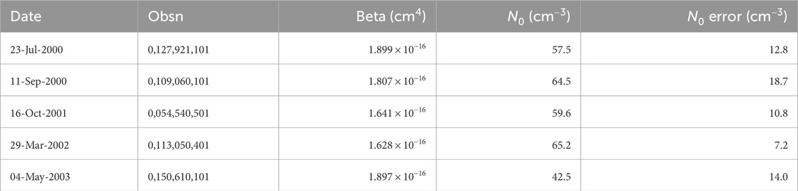
Table 1. Summary of the neutral density estimates in the 5 solar maximum events.

XMM’s primary objective is to study cosmic X-ray sources, and astrophysicists typically remove various background signals from the observed data. These background signals fall into three categories: photons, particles, and electronic noise (Read and Ponman, 2003; Carter and Read, 2007). The photon background includes astrophysical sources, such as thermal emission and emission from unresolved cosmological sources, as well as SWCX from both the heliosphere and exosphere. In our study, we utilized the SWCX background components from the exosphere to estimate ${\text{N}}_0$.

To obtain the SWCX count rates $(C{R}_{\mathit{SWCX}})$ from the exosphere, we removed all other X-ray sources from the raw XMM observations, including the astrophysical, heliospheric, and particle backgrounds, electronic noise, and X-rays from point sources (e.g., stars), using standard XMM software procedures. In our five analyzed events, we found that, on average, approximately 49.9% of the total soft X-ray intensity was attributed to astrophysical sources, 19.6% to the particle backgrounds, 6.0% to the heliospheric SWCX, and 24.5% to exospheric SWCX.

We simulated magnetosheath conditions—specifically plasma number density, velocity, and temperature—for each event using the OpenGGCM MHD model. OpenGGCM simulates the interaction between the solar wind and Earth’s magnetosphere by solving resistive MHD equations on a stretched Cartesian grid. The model’s inputs are solar wind parameters and IMF data from a solar wind monitor, while its outputs include plasma density, velocity, temperature, and electromagnetic fields within the simulation domain. The simulation domain in this study extends from 25 ${\text{R}}_E$ upstream to 500 ${\text{R}}_E$ downstream, with ${\text{Y}}_{\mathit{GSE}}$ and ${\text{Z}}_{\mathit{GSE}}$ domains ranging from −48 to 48 ${\text{R}}_E$. We used a standalone version of OpenGGCM with NASA OMNI solar wind/IMF input data (King and Papitashvili, 2005). More details and applications of the OpenGGCM model can be found in Raeder et al. (2001), Raeder et al. (2008); Connor et al. (2012), Connor et al. (2014), Connor et al. (2015), Connor et al. (2016), Connor et al. (2021); Cramer et al. (2017); Ferdousi and Raeder (2016); Ferdousi et al. (2021); Jensen et al. (2017); Kavosi et al. (2018); Oliveira and Raeder (2015); and Shi et al. (2017).

We derived the exospheric neutral density (${\text{N}}_0$) using the exospheric SWCX count rates $(C{R}_{\mathit{SWCX}})$ and OpenGGCM simulations, following the equation provided by Jung et al. (2022):

$N_0=\frac{4\pi }{\beta \mathrm{\Omega }Q}C{R}_{\mathit{SWCX}}\left[{\text{cm}}^{-3}\right](1)$

where $\mathrm{\Omega }$ represents the XMM MOS field of view in steradians, Q is the soft X-ray emissivity or potential reaction rate between high-charge state solar wind ions and exospheric neutrals in the magnetosheath, $C{R}_{\mathit{SWCX}}$ is the exospheric SWCX count rate observed by XMM, and $\beta$ is an effective scale factor. The definitions of Q and $\beta$ are as follows.

$Q=\int \frac{N_N}{N_0}{N}_p{v}_{\mathit{eff}}ds=\int {\left(\frac{10R_E}{R}\right)}^3{N}_p{v}_{\mathit{eff}}ds\left[{\text{cm}}^{-1}{\text{s}}^{-1}\right](2)$

$v_{\mathit{eff}}=\sqrt{v_p^2+3kT/m}\left[km/s\right]$

$\beta ={\displaystyle \sum _{E_j\in E}}{A}_j\frac{N_{sq}}{N_p}{\sigma }_{sq}{Y}_j\left[{\text{cm}}^4\right]$

Here, $m$ and $k$ represent the proton mass and the Boltzmann constant, respectively. Plasma density $(N_p)$, drift velocity $(v_p)$, and temperature $(T)$ are obtained from the OpenGGCM model. The effective velocity $(v_{\mathit{eff}})$ is the relative velocity between the plasma and a neutral atom; typically, the velocity of neutrals is negligibly small compared to the plasma velocity, so only the plasma velocity is considered.

The term $\beta$ represents the effective area-weighted scale factor for the SWCX process, adjusted for the XMM MOS instrument (Jung et al., 2022). The calculation of $\beta$ takes into account several factors: the effective area $A_j$, the number density of a solar wind ion of species $s$ in charge state $q$ (denoted as $N_{sq}$, in ${\text{cm}}^{-3}$), the charge-exchange (CX) cross section ${\sigma }_{sq}$ (in ${\text{cm}}^2$) for the interaction between $S^{q+}$ and hydrogen, and the photon yield $Y_j$ (the number of photons produced during the transition of $S^{(q-1)+}$). These components were obtained from the data of Koutroumpa et al. (2006). Our $\beta$ values, when converted to the effective scale factor $\alpha$ = ${\sum }_{E_j\in E}{E}_j\frac{N_{sq}}{N_p}{\sigma }_{sq}{Y}_j$, yield $\alpha =6.054\times 10^{-16}$ eV ${\text{cm}}^2$, which is consistent with the value of $6\times 10^{-16}$ eV ${\text{cm}}^2$ from previous studies (Cravens et al., 2001; Whittaker and Sembay, 2016). The specific $\beta$ values used for each observation are noted in Table 1. Since we selected observations with stable solar wind conditions, we assumed a constant effective scale factor. However, for studies focusing on solar active periods, variations in the effective scale factor may need to be considered (Zhang et al., 2022).

In deriving Equation 1, Jung et al. (2022) assumed that the exospheric neutral density is spherically symmetric and inversely proportional to the cube of the radial distance from Earth: $N=N_0{(10R_E/r)}^3$ (Cravens et al., 2001; Connor and Carter, 2019; Fuselier et al., 2010; Fuselier et al., 2020). Zoennchen et al. (2021) reported rare geocoronal observations of the outer exosphere, revealing that the exospheric density above 8 ${\text{R}}_E$ follows an $r^{-3}$ dependency, supporting the validity of our analytical exospheric density model. Additional details on each parameter and their derivation can be found in Jung et al. (2022) and the references therein.

3 XMM case studies

Figure 1A shows the location of XMM on 23 July 2000 when the telescope FOV passes through the dayside magnetosheath. The locations of the magnetopause (red) and bow shock (yellow) were calculated using the models of Shue et al. (1998) and Jelínek et al. (2012), respectively, based on solar wind/IMF conditions from NASA OMNI data. XMM started at the orange dot and moved slightly along the short blue line (almost invisible due to the small motion of XMM During the period of interest), and the black line denotes telescope pointing. During the period of our interest, XMM moved from the coordinates (10.3, −3.5, −15.0) to (10.7, −2.4, −15.5) ${\text{R}}_E$ in the GSE coordinate system. Throughout this motion, the XMM’s look direction was fixed to observe an astronomical object of interest. Figure 1B shows the solar wind/IMF conditions during the event. XMM observation time used in this study is denoted as the green shaded interval, and Geotail’s magnetosheath crossing time is denoted as the gray shaded interval. From top to bottom, IMF, solar wind velocity, density, plasma pressure, and proton flux are shown. During the 2 h XMM observation, the solar wind and IMF were relatively steady except for a brief peak in number density and plasma pressure around 18:20 UT.

Figure 1

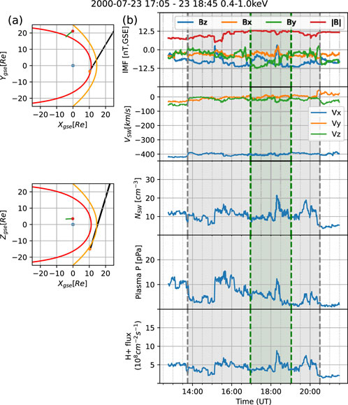
Figure 1. (a) XMM location (blue line starting from orange dot), its pointing direction (black), and the Geotail orbit (green) projected on the GSE XY (top) and XZ (bottom) planes, on 23 July 2000. The starting location of XMM and Geotail are shown as orange and red dots, respectively. The yellow and red curves show the bow shock (Jelínek et al., 2012) and the magnetopause (Shue et al., 1998), respectively. (b) Solar wind and IMF conditions during the XMM observation (green area) and during the Geotail magnetosheath crossing (gray area), obtained from OMNI data. The IMF, solar wind velocity, number density, plasma pressure (=nkT), and solar wind proton flux $(n_{sw}{v}_{sw})$ in the GSE coordinates are shown from top to bottom.

We ran an OpenGGCM simulation to calculate the potential reaction rate Q. To validate the model result, we compared the OpenGGCM results with Geotail (Nishida, 1994) in situ measurements in Figure 2. In top three panels, plasma number density $(N_p)$, effective plasma velocity $(V_{\mathit{eff}})$, effective flux $(N_p\times V_{\mathit{eff}})$ are shown, with the OpenGGCM results (green lines) and Geotail measurements (blue lines). As shown in Equation 1, Q is a crucial factor in obtaining an accurate exospheric density $N_0$ and its value is strongly dependent on the effective flux (see Equation 2). We calculated the model-to-data ratio of the effective flux to assess the discrepancy between the model and observations, and adjust the simulated Q based on this discrepancy. The last panel of Figure 2 displays this ratio in blue. If the model perfectly matched the observations, the ratio would equal 1 and align with the horizontal black line. However, OpenGGCM shows a model-to-data ratio of less than 1, primarily due to a lower plasma density compared to the Geotail observations. We averaged the model-to-data flux ratio during Geotail’s magnetosheath crossing (shaded region) and used this value to adjust Q with the following equation: Q = $Q_{\mathit{MHD}}$/ratio. For the XMM event on 23 July 2000, this average model-to-data ratio is 0.65, leading to an adjustment of Q by dividing Q_MHD by 0.65.

Figure 2

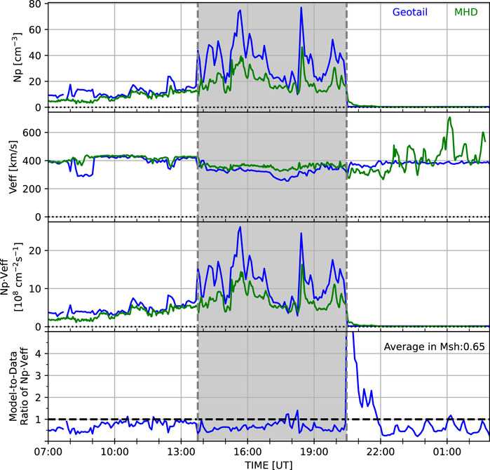
Figure 2. Comparison of the OpenGGCM results (green) with the geotail plasma observation (blue) on 23 July 2000. From top to bottom, the IMF, solar wind velocity, density, plasma pressure, and proton flux are shown. The gray shaded area indicates when Geotail passed through the magnetosheath. The dashed horizontal black line in the bottom panel shows where the model-to-data ratio equals 1.

We also estimated the error in Q due to differences between the modeled and observed magnetosheath boundaries. If the simulated magnetosheath is thicker (or thinner) than observed, the instrument’s line of sight (LOS) within the magnetosheath will be extended (or shortened), resulting in the accumulation of more (or fewer) SWCX photons along the LOS, which could lead to an overestimation or underestimation of Q. We applied the technique of Jung et al. (2022) to calculate this error in Q. This technique adjusts the locations of the magnetopause and bow shock based on boundary crossing observations, and estimates the largest error in Q by calculating the discrepancy between Q values obtained using modeled and adjusted magnetosheath. Figure 2 shows that the boundary crossings of Geotail, marked by the endpoints of the gray shaded area, matches well with the model predictions. As a result, the maximum error in Q for this event was 1.1%.

Figure 3 presents the solar wind flux, the modeled potential reaction rate $(Q_{\mathit{MHD}})$, SWCX count rates observed by XMM (${\text{CR}}_{\mathit{SWCX}}$), and the estimated neutral density at 10 ${\text{R}}_E$ (${\text{N}}_0$) for the XMM event on 23 July 2000. The vertical lines in the bottom two plots represent the error bars for ${\text{CR}}_{\mathit{SWCX}}$ and ${\text{N}}_0$, which were propagated from uncertainties in the count rates and in Q.

Figure 3

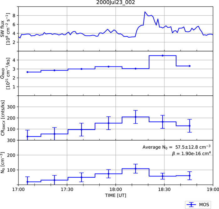
Figure 3. Neutral density estimates for 23 July 2000 event. From top to bottom, solar wind flux, modeled potential reaction rate $(Q_{\mathit{MHD}})$, SWCX count rates observed by XMM $(C{R}_{\mathit{SWCX}})$, and estimated neutral density at 10 ${\text{R}}_E$ (${\text{N}}_0$) are shown.

The error in $C{R}_{\mathit{SWCX}}\mathrm{\Delta }C{R}_{\mathit{SWCX}}$ was determined by propagating the uncertainties from the various background components, including Poisson errors of astrophysical, particle, and heliospheric backgrounds, as detailed in Jung et al. (2022). The error in $Q$ $(\mathrm{\Delta }Q)$ due to the boundary correction is 1.1%, as discussed earlier. The overall error in $N_0$ can be expressed as:

${\left(\frac{\mathrm{\Delta }{N}_0}{N_0}\right)}^2={\left(\frac{\mathrm{\Delta }C{R}_{\mathit{SWCX}}}{C{R}_{\mathit{SWCX}}}\right)}^2+{\left(\frac{\mathrm{\Delta }Q}{Q}\right)}^2$

By applying this approach, we obtained the average neutral density of 60.8 ${\text{cm}}^{-3}$, with an error of 12.2 ${\text{cm}}^{-3}$.

In the first panel of Figure 3, the solar wind flux was mostly steady, with an increase around 18:20 UT. Potential reaction rate Q also follows the same pattern, as expected in Equation 2. SWCX count rates show a similar pattern but the increase happens a bit earlier, around 18:05 UT. The discrepancy between the peaks of ${\text{CR}}_{\mathit{SWCX}}$ and solar wind flux can be partially attributed to variations in the composition of highly charged ions, as observed in ACE SWICS data during the event. While the solar wind flux increased, SWICS measurements showed a decreasing trend in the O/H ratio, from $1.29\times 10^{-4}$ to $1.18\times 10^{-4}$, over the relevant time period. This indicates a reduction in the relative abundance of oxygen lines (${\text{O}}^{6+}$, ${\text{O}}^{7+}$, etc.), which are primary contributors to SWCX emissions. Since SWCX intensity depends directly on the density of highly charged ions, this compositional change could result in an earlier peak in ${\text{CR}}_{\mathit{SWCX}}$ relative to the bulk solar wind flux.

We applied similar techniques to four additional XMM observations. Table 1 shows these observation dates, XMM observation number, effective scale factor $\beta$, estimated neutral density at 10 ${\text{R}}_E$ (${\text{N}}_0$), error of the density estimates (${\text{N}}_0$ Error). As with the 23 July 2000 case, we ran an OpenGGCM simulation for each observation and validated the results using in situ data when available. When in situ data were not present, we utilized the empirical magnetosheath model of Jung et al. (2023) to check whether the OpenGGCM magnetosheath predictions are reasonable. This empirical model showed comparable or better agreement with THEMIS magnetosheath observations compared to other empirical models and was therefore chosen as an alternative for assessing the reliability of the OpenGGCM results. The five XMM case studies estimated exospheric neutral densities ranging from 42.5 to 65.2 ${\text{cm}}^{-3}$, with uncertainties of 7–19 ${\text{cm}}^{-3}$.

4 Discussion

Our exospheric neutral density estimates are consistent with previous X-ray studies. Connor and Carter (2019) derived neutral densities at 10 ${\text{R}}_E$ from two XMM observations in 2001 and 2003, reporting values of 39.9 ${\text{cm}}^{-3}$ and 57.6 ${\text{cm}}^{-3}$, respectively. Jung et al. (2022) estimated a density of 36.8 $\pm$ 11.7 ${\text{cm}}^{-3}$ based on an XMM observation in 2008.

Recent Lyman-$\alpha$ studies have also reported similar density estimates: Kameda et al. (2017) used the LAICA instrument to image the exosphere and derived hydrogen density distributions by fitting the data to a modified Chamberlain-type model that accounts for solar radiation pressure. Cucho-Padin et al. (2022) employed an inverse problem solution that uses the Kameda model as prior knowledge while allowing greater freedom in the retrieved densities, reporting a value of 26.51 ${\text{cm}}^{-3}$ at 10 ${\text{R}}_E$. Baliukin et al. (2019) estimated approximately 60 ${\text{cm}}^{-3}$ at 10 ${\text{R}}_E$ using SOHO/SWAN (Solar and Heliospheric Observatory/Solar Wind Anisotropies) data, while Zoennchen et al. (2021) reported a density of 35 ${\text{cm}}^{-3}$ based on CASSINI Lyman-$\alpha$ observations during its transit to Earth. These density measurements from various studies are summarized in Table 2 for comparison. These values fall within the margin of error of our estimates.

Table 2

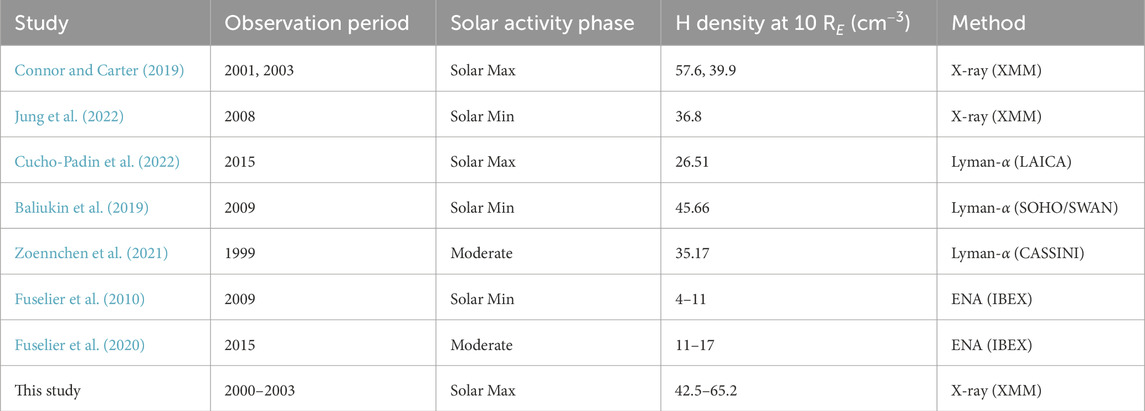
Table 2. Comparison of exospheric H density estimates at 10 ${\text{R}}_E$ from various studies.

However, our results differ from those based on Energetic Neutral Atom (ENA) observations. ENAs form when solar wind protons exchange electrons with exospheric hydrogen atoms. Fuselier et al. (2010), Fuselier et al. (2020) derived neutral densities at 10 ${\text{R}}_E$ from IBEX (Interstellar Boundary Explorer) ENA observations of Earth’s magnetosheath, using time-dependent homogeneous or gasdynamic magnetosheath models. Their estimates range from 4 to 17 ${\text{cm}}^{-3}$, significantly lower than those from X-ray and Lyman-$\alpha$ studies. Sibeck et al. (2021) suggested that these ENA-based densities might increase with the application of more advanced magnetosheath models, a topic for future research.

The influence of solar activity on exospheric density remains an active area of investigation. Geocoronal observations from the Two Wide-angle Imaging Neutral-atom Spectrometers (TWINS) spacecraft suggest higher densities at 3–8 ${\text{R}}_E$ during solar maximum conditions (Zoennchen et al., 2015). In contrast, SOHO/SWAN data indicate decreased hydrogen densities at a tangential distance of 7 ${\text{R}}_E$ during solar maximum (Baliukin et al., 2019).

Our study builds on Jung et al. (2022), who derived a density of 36.8 $\pm$ 11.7 ${\text{cm}}^{-3}$ at the subsolar point at 10 ${\text{R}}_E$ from XMM observations during the solar minimum of November 2008. In comparison, our analysis during solar maximum conditions estimates densities between 42.5 and 65.2 ${\text{cm}}^{-3}$ at 10 ${\text{R}}_E$.

These results indicate a trend of higher exospheric densities during solar maximum compared to solar minimum, consistent with TWINS observations. However, given the overlapping error bars, the difference between solar maximum and minimum values appears modest, suggesting a minimal solar cycle impact on exospheric density. Further statistical studies are needed to confirm variations in neutral density across the solar cycle.

5 Conclusion

We estimated exospheric neutral density at the subsolar location at 10 ${\text{R}}_E$ using five XMM observations during solar maximum, applying the technique of Jung et al. (2022). The exospheric SWCX signal was isolated from other soft X-ray background components, and the OpenGGCM simulation was run for each event to calculate the potential reaction rate, Q. Using the obtained SWCX signal and Q, the neutral density was estimated using Equation 1, resulting in a density range of 42.5–65.2 ${\text{cm}}^{-3}$ at the 10 ${\text{R}}_E$ subsolar point, with errors of 7.2–14.0 ${\text{cm}}^{-3}$. This result is consistent with previous studies, including Zoennchen et al. (2021), which reported a density of 35.17 ${\text{cm}}^{-3}$ (with a 25% error), Connor and Carter (2019), which estimated a range of 39.9–57.6 ${\text{cm}}^{-3}$, and Jung et al. (2022), which provided a density of 36.8 $\pm$ 11.7 ${\text{cm}}^{-3}$.

The soft X-ray telescopes onboard the LEXI and SMILE missions will study the global interaction between the solar wind and Earth’s magnetospheric system by imaging the magnetosheath boundary and its motion in soft X-rays. The density of exospheric hydrogen is a critical parameter influencing the strength of magnetosheath SWCX signals. Numerical simulations by Sibeck et al. (2018) demonstrated that magnetosheath SWCX signals can be readily distinguished from other soft X-ray background emission if the exospheric density is at least 22 ${\text{cm}}^{-3}$ at a radial distance of 9.74 ${\text{R}}_E$.

Previous mission studies (e.g., Connor et al., 2021; Sun et al., 2019; Samsonov et al., 2023) have commonly used 25 ${\text{cm}}^{-3}$ as the exospheric density at the subsolar location of 10 ${\text{R}}_E$ for simulating soft X-ray images of Earth’s magnetosphere. Our density estimates, which are higher than these assumed values, suggest stronger SWCX signals in the dayside magnetosheath. This is encouraging news for the LEXI and SMILE missions, which are set to launch during the solar maximum period in 2025.

Data availability statement

The datasets presented in this study can be found in online repositories. The names of the repository/repositories and accession number(s) can be found below: https://github.com/jjung11/XMM2025.

Author contributions

JJ: Conceptualization, Data curation, Formal Analysis, Investigation, Methodology, Project administration, Resources, Software, Validation, Visualization, Writing – original draft, Writing – review and editing. HC: Conceptualization, Funding acquisition, Project administration, Supervision, Writing – review and editing. JC: Conceptualization, Data curation, Methodology, Supervision, Validation, Writing – review and editing. DK: Resources, Writing – review and editing. CP: Methodology, Resources, Writing – review and editing.

Funding

The author(s) declare that financial support was received for the research and/or publication of this article. This work was supported by the NSF grant AGS-1928883 and the NASA grants, 80NSSC18K1043 and 80NSSC20K1670, 80MSFC20C0019, WBS 516741.01.24.01.03, and WBS 791926.02.04.02.26. JAC is supported by Royal Society grant DHF∖R1∖211,068.

Conflict of interest

The authors declare that the research was conducted in the absence of any commercial or financial relationships that could be construed as a potential conflict of interest.

Generative AI statement

The author(s) declare that no Gen AI was used in the creation of this manuscript.

Publisher’s note

All claims expressed in this article are solely those of the authors and do not necessarily represent those of their affiliated organizations, or those of the publisher, the editors and the reviewers. Any product that may be evaluated in this article, or claim that may be made by its manufacturer, is not guaranteed or endorsed by the publisher.

References

Angelopoulos, V. (2009). The THEMIS mission. Springer.

Google Scholar

Baliukin, I. I., Bertaux, J.-L., Quémerais, E., Izmodenov, V., and Schmidt, W. (2019). Swan/soho lyman-α mapping: the hydrogen geocorona extends well beyond the moon. J. Geophys. Res. Space Phys. 124, 861–885. doi:10.1029/2018ja026136

CrossRef Full Text | Google Scholar

Branduardi-Raymont, G., Wang, C., Dai, L., Donovan, E., Li, L., and Sembay, S. (2018). Smile definition study report. ESA/SCI 2018, 1. doi:10.5270/esa.smile.definition_study_report-2018-12

CrossRef Full Text | Google Scholar

Burch, J., Moore, T., Torbert, R., and Giles, B.-h. (2016). Magnetospheric multiscale overview and science objectives. Space Sci. Rev. 199, 5–21. doi:10.1007/978-94-024-0861-4_2

CrossRef Full Text | Google Scholar

Carter, J., and Read, A. (2007). The xmm-Newton epic background and the production of background blank sky event files. Astronomy and Astrophysics 464, 1155–1166. doi:10.1051/0004-6361:20065882

CrossRef Full Text | Google Scholar

Carter, J., Sembay, S., and Read, A. (2010). A high charge state coronal mass ejection seen through solar wind charge exchange emission as detected by xmm–Newton. Mon. Notices R. Astronomical Soc. 402, 867–878. doi:10.1111/j.1365-2966.2009.15985.x

CrossRef Full Text | Google Scholar

Carter, J., Sembay, S., and Read, A. (2011). Identifying xmm-Newton observations affected by solar wind charge exchange–part ii. Astronomy and Astrophysics 527, A115. doi:10.1051/0004-6361/201015817

CrossRef Full Text | Google Scholar

Collier, M., Abbey, T., Bannister, N., Carter, J., Choi, M., Cravens, T., et al. (2009). The lunar x-ray observatory (lxo)/magnetosheath explorer in x-rays (magex). AIP Conf. Proc. Am. Inst. Phys. 1156, 105–111. doi:10.1063/1.3211802

CrossRef Full Text | Google Scholar

Connor, H., and Carter, J. A. (2019). Exospheric neutral hydrogen density at the nominal 10 R_E subsolar point deduced from XMM-Newton X-ray observations. J. Geophys. Res. Space Phys. 124, 1612–1624. doi:10.1029/2018ja026187

CrossRef Full Text | Google Scholar

Connor, H., Raeder, J., Sibeck, D., and Trattner, K. (2015). Relation between cusp ion structures and dayside reconnection for four imf clock angles: openggcm-ltpt results. J. Geophys. Res. Space Phys. 120, 4890–4906. doi:10.1002/2015ja021156

CrossRef Full Text | Google Scholar

Connor, H., Raeder, J., and Trattner, K. (2012). Dynamic modeling of cusp ion structures. J. Geophys. Res. Space Phys. 117. doi:10.1029/2011ja017203

CrossRef Full Text | Google Scholar

Connor, H., Sibeck, D., Collier, M., Baliukin, I., Branduardi-Raymont, G., Brandt, P., et al. (2021). Soft x-ray and ena imaging of the earth’s dayside magnetosphere. J. Geophys. Res. Space Phys. 126, e2020JA028816. doi:10.1029/2020ja028816

PubMed Abstract | CrossRef Full Text | Google Scholar

Connor, H., Zesta, E., Fedrizzi, M., Shi, Y., Raeder, J., Codrescu, M. V., et al. (2016). Modeling the ionosphere-thermosphere response to a geomagnetic storm using physics-based magnetospheric energy input: openggcm-ctim results. J. Space Weather Space Clim. 6, A25. doi:10.1051/swsc/2016019

CrossRef Full Text | Google Scholar

Connor, H., Zesta, E., Ober, D., and Raeder, J. (2014). The relation between transpolar potential and reconnection rates during sudden enhancement of solar wind dynamic pressure: openggcm-ctim results. J. Geophys. Res. Space Phys. 119, 3411–3429. doi:10.1002/2013ja019728

CrossRef Full Text | Google Scholar

Cramer, W. D., Raeder, J., Toffoletto, F., Gilson, M., and Hu, B. (2017). Plasma sheet injections into the inner magnetosphere: two-way coupled openggcm-rcm model results. J. Geophys. Res. Space Phys. 122, 5077–5091. doi:10.1002/2017ja024104

CrossRef Full Text | Google Scholar

Cravens, T., Robertson, I., and Snowden, S. (2001). Temporal variations of geocoronal and heliospheric x-ray emission associated with the solar wind interaction with neutrals. J. Geophys. Res. Space Phys. 106, 24883–24892. doi:10.1029/2000ja000461

CrossRef Full Text | Google Scholar

Cucho-Padin, G., Kameda, S., and Sibeck, D. G. (2022). The earth’s outer exospheric density distributions derived from procyon/laica uv observations. J. Geophys. Res. Space Phys. 127, e2021JA030211. doi:10.1029/2021ja030211

CrossRef Full Text | Google Scholar

de la Calle, I. (2021). Users guide of the xmm-Newton science analysis system. 16.0, 2021 (ESA: XMM-Newton SOC)

Google Scholar

Dimmock, A., and Nykyri, K. (2013). The statistical mapping of magnetosheath plasma properties based on themis measurements in the magnetosheath interplanetary medium reference frame. J. Geophys. Res. Space Phys. 118, 4963–4976. doi:10.1002/jgra.50465

CrossRef Full Text | Google Scholar

Escoubet, C., Fehringer, M., and Goldstein, M. (2001). IntroductionThe cluster mission. Ann. Geophys. Copernic. GmbH 19, 1197–1200. doi:10.5194/angeo-19-1197-2001

CrossRef Full Text | Google Scholar

Ferdousi, B., and Raeder, J. (2016). Signal propagation time from the magnetotail to the ionosphere: openggcm simulation. J. Geophys. Res. Space Phys. 121, 6549–6561. doi:10.1002/2016ja022445

CrossRef Full Text | Google Scholar

Ferdousi, B., Raeder, J., Zesta, E., Cramer, W., and Murphy, K. (2021). Association of auroral streamers and bursty bulk flows during different states of the magnetotail: a case study. J. Geophys. Res. Space Phys. 126, e2021JA029329. doi:10.1029/2021ja029329

CrossRef Full Text | Google Scholar

Fuselier, S., Dayeh, M., Galli, A., Funsten, H., Schwadron, N., Petrinec, S., et al. (2020). Neutral atom imaging of the solar wind-magnetosphere-exosphere interaction near the subsolar magnetopause. Geophys. Res. Lett. 47, e2020GL089362. doi:10.1029/2020gl089362

PubMed Abstract | CrossRef Full Text | Google Scholar

Fuselier, S., Funsten, H., Heirtzler, D., Janzen, P., Kucharek, H., McComas, D., et al. (2010). Energetic neutral atoms from the earth’s subsolar magnetopause. Geophys. Res. Lett. 37. doi:10.1029/2010gl044140

CrossRef Full Text | Google Scholar

Jansen, F., Lumb, D., Altieri, B., Clavel, J., Ehle, M., Erd, C., et al. (2001). Xmm-Newton observatory-i. the spacecraft and operations. Astronomy and Astrophysics 365, L1–L6. doi:10.1051/0004-6361:20000036

CrossRef Full Text | Google Scholar

Jelínek, K., Němeček, Z., and Šafránková, J. (2012). A new approach to magnetopause and bow shock modeling based on automated region identification. J. Geophys. Res. Space Phys. 117. doi:10.1029/2011ja017252

CrossRef Full Text | Google Scholar

Jensen, J. B., Raeder, J., Maynard, K., and Cramer, W. D. (2017). Particle precipitation effects on convection and the magnetic reconnection rate in earth’s magnetosphere. J. Geophys. Res. Space Phys. 122, 11–413. doi:10.1002/2017ja024030

CrossRef Full Text | Google Scholar

Jung, J., Connor, H., Dimmock, A., Sembay, S., Read, A., and Soucek, J. (2023). Mshpy23: a user-friendly, parameterized model of magnetosheath conditions. Phys. Earth Planet. Interiors 8, 89–104. doi:10.26464/epp2023065

CrossRef Full Text | Google Scholar

Jung, J., Connor, H. K., Carter, J. A., Koutroumpa, D., Pagani, C., and Kuntz, K. (2022). Solar minimum exospheric neutral density near the subsolar magnetopause estimated from the xmm soft x-ray observations on 12 november 2008. J. Geophys. Res. Space Phys. 127, e2021JA029676. doi:10.1029/2021ja029676

CrossRef Full Text | Google Scholar

Kameda, S., Ikezawa, S., Sato, M., Kuwabara, M., Osada, N., Murakami, G., et al. (2017). Ecliptic north-south symmetry of hydrogen geocorona. Geophys. Res. Lett. 44, 11–706. doi:10.1002/2017gl075915

CrossRef Full Text | Google Scholar

Kavosi, S., Spence, H., Fennell, J., Turner, D., Connor, H., and Raeder, J. (2018). Mms/feeps observations of electron microinjections due to kelvin-helmholtz waves and flux transfer events: a case study. J. Geophys. Res. Space Phys. 123, 5364–5378. doi:10.1029/2018ja025244

CrossRef Full Text | Google Scholar

King, J., and Papitashvili, N. (2005). Solar wind spatial scales in and comparisons of hourly wind and ace plasma and magnetic field data. J. Geophys. Res. Space Phys. 110. doi:10.1029/2004ja010649

CrossRef Full Text | Google Scholar

Koutroumpa, D., Lallement, R., Kharchenko, V., Dalgarno, A., Pepino, R., Izmodenov, V., et al. (2006). Charge-transfer induced euv and soft x-ray emissions in the heliosphere. Astronomy and Astrophysics 460, 289–300. doi:10.1051/0004-6361:20065250

CrossRef Full Text | Google Scholar

[Dataset] Nishida, A. (1994). The geotail mission. Geophys. Res. Lett. 21, 2871–2873. doi:10.1029/94gl01223

CrossRef Full Text | Google Scholar

Oliveira, D. M., and Raeder, J. (2015). Impact angle control of interplanetary shock geoeffectiveness: a statistical study. J. Geophys. Res. Space Phys. 120, 4313–4323. doi:10.1002/2015ja021147

CrossRef Full Text | Google Scholar

Raeder, J., Larson, D., Li, W., Kepko, E. L., and Fuller-Rowell, T. (2008). Openggcm simulations for the themis mission. Space Sci. Rev. 141, 535–555. doi:10.1007/s11214-008-9421-5

CrossRef Full Text | Google Scholar

Raeder, J., McPherron, R., Frank, L., Kokubun, S., Lu, G., Mukai, T., et al. (2001). Global simulation of the geospace environment modeling substorm challenge event. J. Geophys. Res. Space Phys. 106, 381–395. doi:10.1029/2000ja000605

CrossRef Full Text | Google Scholar

Read, A. M., and Ponman, T. J. (2003). The xmm-Newton epic background: production of background maps and event files. Astronomy and Astrophysics 409, 395–410. doi:10.1051/0004-6361:20031099

CrossRef Full Text | Google Scholar

Samsonov, A., Branduardi-Raymont, G., Sembay, S., Read, A., Sibeck, D., and Rastaetter, L. (2023). Simulation of the smile soft x-ray imager response to a southward interplanetary magnetic field turning. Earth Planet. Phys. 8, 39–46. doi:10.26464/epp2023058

CrossRef Full Text | Google Scholar

Shi, Y., Zesta, E., Connor, H., Su, Y.-J., Sutton, E., Huang, C., et al. (2017). High-latitude thermosphere neutral density response to solar wind dynamic pressure enhancement. J. Geophys. Res. Space Phys. 122, 11–559. doi:10.1002/2017ja023889

CrossRef Full Text | Google Scholar

Shue, J.-H., Song, P., Russell, C., Steinberg, J., Chao, J., Zastenker, G., et al. (1998). Magnetopause location under extreme solar wind conditions. J. Geophys. Res. Space Phys. 103, 17691–17700. doi:10.1029/98ja01103

CrossRef Full Text | Google Scholar

Sibeck, D., Collier, M., and Silveira, M. (2021). Neutral densities in the outer exosphere near the subsolar magnetopause. Geophys. Res. Lett. 48, e2021GL093383. doi:10.1029/2021gl093383

CrossRef Full Text | Google Scholar

Sibeck, D. G., Allen, R., Aryan, H., Bodewits, D., Brandt, P., Branduardi-Raymont, G., et al. (2018). Imaging plasma density structures in the soft x-rays generated by solar wind charge exchange with neutrals. Space Sci. Rev. 214, 79–124. doi:10.1007/s11214-018-0504-7

CrossRef Full Text | Google Scholar

Snowden, S., Collier, M., and Kuntz, K. (2004). Xmm-Newton observation of solar wind charge exchange emission. Astrophysical J. 610, 1182–1190. doi:10.1086/421841

CrossRef Full Text | Google Scholar

Sun, T., Wang, C., Sembay, S., Lopez, R., Escoubet, C., Branduardi-Raymont, G., et al. (2019). Soft x-ray imaging of the magnetosheath and cusps under different solar wind conditions: mhd simulations. J. Geophys. Res. Space Phys. 124, 2435–2450. doi:10.1029/2018ja026093

CrossRef Full Text | Google Scholar

Turner, M. J., Abbey, A., Arnaud, M., Balasini, M., Barbera, M., Belsole, E., et al. (2001). The european photon imaging camera on xmm-Newton: the mos cameras. Astronomy and Astrophysics 365, L27–L35. doi:10.1051/0004-6361:20000087

CrossRef Full Text | Google Scholar

Walsh, B., Kuntz, K., Busk, S., Cameron, T., Chornay, D., Chuchra, A., et al. (2024). The lunar environment heliophysics x-ray imager (lexi) mission. Space Sci. Rev. 220, 37–27. doi:10.1007/s11214-024-01063-4

PubMed Abstract | CrossRef Full Text | Google Scholar

Walsh, B., Kuntz, K., Collier, M., Sibeck, D., Snowden, S., and Thomas, N. (2014). Energetic particle impact on x-ray imaging with xmm-Newton. Space weather. 12, 387–394. doi:10.1002/2014sw001046

CrossRef Full Text | Google Scholar

Whittaker, I. C., and Sembay, S. (2016). A comparison of empirical and experimental o7+, o8+, and o/h values, with applications to terrestrial solar wind charge exchange. Geophys. Res. Lett. 43, 7328–7337. doi:10.1002/2016gl069914

CrossRef Full Text | Google Scholar

Zhang, Y., Sun, T., Wang, C., Ji, L., Carter, J. A., Sembay, S., et al. (2022). Solar wind charge exchange soft x-ray emissions in the magnetosphere during an interplanetary coronal mass ejection compared to its driven sheath. Astrophysical J. Lett. 932, L1. doi:10.3847/2041-8213/ac7521

CrossRef Full Text | Google Scholar

Zoennchen, J., Nass, U., and Fahr, H. (2015). Terrestrial exospheric hydrogen density distributions under solar minimum and solar maximum conditions observed by the twins stereo mission. Ann. Geophys. Copernic. GmbH 33, 413–426. doi:10.5194/angeo-33-413-2015

CrossRef Full Text | Google Scholar

Zoennchen, J. H., Connor, H. K., Jung, J., Nass, U., and Fahr, H. J. (2021). Terrestrial exospheric dayside h-density profile at 3–15 r e from uvis/hdac and twins lyman-α data combined. Ann. Geophys. Discuss. 2021, 1–16. doi:10.5194/angeo-40-271-2022

CrossRef Full Text | Google Scholar