A method to localize plasma density enhancements along lines of sight to radio sources through PSP/WISPR’s field of view

Introduction: Coronal Faraday rotation (FR) measurements provide a powerful means of measuring the magnetic field of the solar corona and solar wind (along the line of sight (LOS) between a background linearly polarized radio transmitter and a ground-based radio receiver). FR is a path integrated quantity depending on both the plasma density $(n_e)$ and the magnetic field component along the LOS $({\vec{B}}_{\mathit{LOS}})$. Consequently, the fundamental calibration challenge encountered when using radio FR observations to infer the magnetic field structure of the solar wind is distinguishing between the $n_e$ and ${\vec{B}}_{\mathit{LOS}}$ contributions to the detectable FR.

Methods: The method presented here, however, will be able to provide localized plasma density information to FR observations for the first time. Using a synthetic field of view of the Wide-field Imager for Parker Solar Probe (WISPR), we perform a tomographic reconstruction of the plasma density in the vicinity of spacecraft.

Discussion: This article develops the framework to determine the positions, along LOS to radio sources, of the density enhancements we reconstruct tomographically.

Conclusion: While still in development, this method provides the necessary foundation to complement and enhance coronal FR measurements, but the applicability of this technique extends beyond coronal FR.

1 Introduction

In the solar corona and solar wind, our understanding of fundamental phenomena remains incomplete. What processes are responsible for the heating of the corona to millions of Kelvin? What are the sources of the solar wind? What processes drive the acceleration of the solar wind to supersonic speeds? How and under what conditions do heliospheric structures form and evolve? How is the magnetic field structured in the corona and solar wind? What size and time scales dominate different regions of the corona and solar wind? These questions comprise just a handful of the outstanding questions in the field of heliophysics (e.g., see Viall and Borovsky, 2020).

We do know that the coronal magnetic field plays a major role in connecting the Sun to the greater solar system. Within the corona itself, a transition occurs from a magnetically dominated regime to a thermally dominated regime, at heliocentric distances of $\sim 3{\mathrm{R}}_{\odot }$ (Newkirk, 1967). Many models of coronal heating and solar wind acceleration depend on magnetic field and plasma structure below $5{\mathrm{R}}_{\odot }$ (McComas et al., 2007). However, remote sensing techniques still comprise the only means of probing these regions of the heliosphere. Even in a new era of heliophysics, wherein Parker Solar Probe (PSP, Fox et al., 2016) and Solar Orbiter (SO, Müller et al., 2020) fly through the plasma of the inner heliosphere and sample it directly, we still lack consistent in situ access to the poles, the corona below $10{\mathrm{R}}_{\odot }$, and all regions outside the orbital paths of these spacecraft.

Nonetheless, PSP and SO offer abundant new insights and questions as they fly through the inner heliosphere, past and through the very structures we wish to investigate. In particular, the heliospheric imagers onboard these spacecraft–the Wide-field Imager for Parker Solar Probe (WISPR, Vourlidas et al., 2016) and the Solar Orbiter Heliospheric Imager (Howard et al., 2020) – image the corona and solar wind at unprecedented sensitivity and spatial resolution.

It is important to observe long-lived, large-scale, quasi-radial features in the corona and solar wind, as they illuminate underlying structuring processes and the interplay of magnetism and plasma physics (Golub and Pasachoff, 2010). Coronal streamers are ubiquitous throughout all phases of the solar cycle, appearing in white-light coronagraphs, eclipse images, and heliospheric images when direct light from the far brighter photosphere is sufficiently attenuated. Bipolar (i.e., helmet) streamers consist of open magnetic field lines overlying closed magnetic loops, with a neutral current sheet separating the regions of opposite polarity (Pneuman and Kopp, 1971). Compared to the ‘background’ plasma, streamers are enhanced in density by a factor of $\sim$3 to 10 (Priest, 2012; Athay, 1976). Tracing out the coronal magnetic field structure and heliospheric current sheet, streamers and their fine-scale filamentary structure are of great relevance to many fundamental questions. Additionally, with PSP embedded in the solar corona, WISPR views these coronal structures as it flies towards and past them, seeing them before other PSP instruments detect in situ. With unprecedented spatial resolution come new observations and new questions; regarding the striations that pervade WISPR images, Howard et al. (2022) query: “are these rays simply density enhancements or undulations that are the result of small folds in the heliospheric plasma sheet?”

Recent work by Kenny et al. (2023) and Kenny et al. (2024) has utilized near-perihelion, synthetic WISPR images to reconstruct density structure in the proximity of the spacecraft. This technique, called “translational tomography,” takes advantage of WISPR’s broad range of viewing angles over a short period of time to reconstruct plasma density structure around the spacecraft. These reconstructions are useful for understanding the scale range of coronal inhomogeneities (e.g., DeForest et al., 2018) and also for providing large-scale context for in situ analyses (Kenny et al., 2024).

Furthermore, tracking the intersections of density enhancements with different paths or traces through the corona would promote progress in several different areas of study. We could determine what structures comet trajectories intersect and improve the extent to which an entire field of study–coronal propagation effects–infers physical properties of the corona. Interplanetary scintillation, angular broadening, and Faraday rotation are all part of this class of remote sensing techniques. As plane radio waves traverse the inhomogenous corona and solar wind, they are distorted. We can quantify these effects on the radio signal along a line of sight (LOS) from source to observer and thereby estimate properties of the intervening plasma, including magnetic field, plasma density, and solar wind speed. All coronal propagation studies utilize LOS measurements of the coronal plasma; therefore, these techniques would greatly benefit from any information on the structure and inhomogeneities present along the LOS (to background sources) during observations. To demonstrate the utility of this new method, this article will focus on the plasma propagation effect of Faraday rotation (FR), which requires detailed information about the intervening electron plasma density structure in order to provide sensitive estimates for the plasma’s magnetic field.

Measurements of coronal Faraday rotation (FR) have long been considered one of the best remote sensing methods with which we can infer the LOS magnetic field in the solar corona and solar wind. The Zeeman effect¹ is a powerful tool with which to measure the solar magnetic field vector, from the photosphere into the low corona (e.g., to $\sim 1.2R_{\odot }$; Schad et al., 2024). Other techniques–including radio, polarimetric, and seismological methods–can provide magnetic field diagnostics in the low corona. For example, Yang et al. (2024) performed two-dimensional coronal seismology with over 8 months to make magnetic field measurements from $1.05-1.6R_{\odot }$. However, it is FR that can probe the magnetic field strength and direction in the middle and outer corona, from $\sim 1.5-25R_{\odot }$ (Kooi et al., 2022). FR is a remote-sensing method by which we measure the rotation of the plane of polarization ($\mathrm{\Delta }\chi$, i.e., the change in polarization position angle) of a polarized radiation source. As we see in the following equation for FR, $\mathrm{\Delta }\chi$, the integrand contains the product of the electron plasma density, $n_e$, and the LOS magnetic field, $\vec{B}\cdot d\vec{s}$ (i.e., ${\vec{B}}_{\mathit{LOS}}$).

$\mathrm{\Delta }\chi =\left[\left(\frac{{\mathrm{e}}^{\mathrm{3}}}{8{\mathrm{\pi }}^{\mathrm{2}}{\mathrm{ϵ}}_{\mathrm{0}}{\mathrm{m}}_{\mathrm{e}}^{\mathrm{2}}{\mathrm{c}}^{\mathrm{3}}}\right){\int }_{\mathit{LOS}}{n}_e\vec{B}\cdot \overrightarrow{ds}\right]{\lambda }^2=\left[\text{RM}\right]{\lambda }^2(1)$

The term in parentheses, the FR constant, is comprised of physical constants and numbers: $\mathrm{e}$ is the charge of an electron, ${\mathrm{ϵ}}_{\mathrm{0}}$ is the permittivity of free space, ${\mathrm{m}}_{\mathrm{e}}$ is the mass of an electron, and $\mathrm{c}$ is the speed of light. The FR constant times the LOS integral comprises the rotation measure (RM), which is the physical quantity of FR (in brackets) that is independent of the observational wavelength, $\lambda$. As such, FR observations conducted at multiple frequencies are given in the form of a RM, with SI units of $\mathrm{r}\mathrm{a}\mathrm{d}{\mathrm{m}}^{-\mathrm{2}}$. From the RM, we can infer the LOS magnetic field if and only if we can disentangle the contribution of the (LOS-varying) plasma density. As per Kooi et al. (2022), there are multiple ways to provide contemporaneous information on the plasma density contribution in order to infer the magnetic field contribution: 1) use empirical models for both $n_e$ and $\vec{B}$, 2) use independent data for $n_e$, or 3) combine the two approaches.

If we choose to model the plasma structure in order to disambiguate the contributions of $n_e$ and $\vec{B}$ to the measured RM, the standard practice is to select a formula–either a simple analytic form or an empirically determined form–for $n_e$ and $\vec{B}$ and to iterate the models until they agree with observations, (e.g., Pätzold et al., 1987; Mancuso and Spangler, 2000; Spangler, 2005; Ingleby et al., 2007). Plasma density models come from various datasets ascertained prior to the FR observations, and it is necessary that they match the observations (Pätzold et al., 1987). It is typical to select an appropriate power-law form for both plasma density and magnetic field and fit the coefficients and power-law indices to the FR data (Kooi et al., 2022). The choice of power-law model depends on the impact parameter for a given LOS (i.e., the heliocentric distance to the proximate point along the LOS), the regions of the corona (and coronal morphology) that the many LOS pierce, and the phase of the solar cycle. For more details on the different models used to determine plasma density, please refer to Section 2 of Kooi et al. (2022).

Regardless of which $n_e$ and $\vec{B}$ models are used, the most important parameter to determine in modeling the FR is the intersection point of the line of sight with the heliospheric current sheet (HCS), known as ${\beta }_C$. It is typical to project the radio lines of sight onto a potential-field source surface (PFSS) synoptic chart corresponding to the Carrington rotation during which the observations took place to determine ${\beta }_C$ (Kooi et al., 2022). However, the location of the neutral line can evolve appreciably during a single Carrington rotation and between Carrington rotations. For example, in Table 3 of Kooi et al. (2014), they show how the use of the PFSS synoptic charts for two separate Carrington rotation synoptic charts on either side of the observations results in a difference of nearly $10°$ in ${\beta }_C$. Errors in determining the position of the HCS in relation to the LOS result in errors of $\sim 25\%$ in inferring the magnetic field (You et al., 2012). In summary, we can estimate the intersection point of the LOS with the magnetic neutral line in the heliosphere using empirical models of the plasma density and magnetic field structure during our FR observations, albeit with a large degree of uncertainty in the intersection point ${\beta }_C$.

If we choose to instead use contemporaneous data to supply independent plasma density information, the source of radio emission determines which data are most appropriate. For pulsars, we use dispersion measurements; for spacecraft beacons, we use radio ranging and apparent-Doppler tracking; and for radio galaxies, we use Thomson scattering brightness measurements. We conducted FR observations during PSP Perihelia 15, 16, and 22, which possess the right Earth-PSP geometry to use the new WISPR-enhanced calibration and analysis described in this article. All three of these observations utilize radio galaxies as the background sources of radio waves. As such, we will describe how one can use Thomson scattering brightness (TSB) measurements to determine $n_e$. For a detailed description of methods used to determine $n_e$ for FR observations involving millisecond pulsars and background spacecraft as the sources of radio signals, see You et al. (2012) and Jensen et al. (2016) respectively.

For LOS with solar offsets beyond the outer edge of a coronagraph’s occulting disk (e.g., $\sim 2R_{\odot }$ for SOHO/LASCO’s C2 coronagraph (Brueckner et al., 1995)), one can use coronagraph images to determine the TSB and consequently the plasma density. Because the TSB is the brightness of photospheric emission scattered off electrons with the corona, we can back out the density of electrons–the dominant constituent of the coronal and solar wind plasma–by measuring the TSB. As Equation 2 shows, TSB is a LOS integral of the plasma density times a geometric factor, which are both a function of heliocentric distance:

$TSB={\int }_{\mathit{LOS}}{n}_e\left(\vec{r}\right)\mathcal{G}\left(\vec{r}\right)dr(2)$

where $\vec{r}$ is the heliocentric distance, and $\mathcal{G}(\vec{r})$ is a geometric function that incorporates solar limb darkening and heliocentric distance assumptions (van de Hulst, 1950; Hayes et al., 2001). The full form for $\mathcal{G}(\vec{r})$ can be found in van de Hulst (1950). It is not trivial to determine the TSB from the coronagraph images. In addition to the K corona (photospheric light scattering off coronal electrons), the F-corona (photospheric light scattering off interplanetary dust) also contributes to the total brightness in coronagraph images. It is therefore necessary to subtract off the brightness contribution from the F-corona. The accuracy with which we can remove the F-corona contribution determines the accuracy with which we can derive the plasma density from total brightness observations (Hayes et al., 2001).

Regardless of the data used to estimate $n_e$, a fundamental issue plagues the approach: none of these methods returns information on how the plasma density varies along the line of sight. Dispersion measurements, radio ranging and apparent-Doppler tracking, and Thomson scattering brightness measurements are all integrated quantities and thus return the sum of $n_e$ over the entire line of sight. In order to improve the sensitivity with which we estimate ${\vec{B}}_{\mathit{LOS}}$ from FR measurements, it is necessary to improve our $n_e$ techniques. Presently, there exist techniques to determine positional information on the coronal plasma, which can be used to improve magnetic field retrieval from FR measurements.

For example, Jackson et al. (2020) (and references therein) reconstruct three-dimensional, time-dependent information on coronal plasma parameters. Their technique combines three-dimensional models of the solar wind and data from interplanetary scintillation (IPS), Thomson scattering brightness, or a combination of both to iteratively characterize not only co-rotating features but also coronal mass ejections (CMEs). This tomographic method performs least-squares fitting of two solar wind parameters (density and radial velocity) until the solar wind model matches observed quantities, both at a source surface (the model boundary) and in three dimensions (Jackson et al., 2020). Assumptions embedded in the technique include weak scattering (such that the LOS-integrated IPS measurement at Earth may be considered a sum of contributions from thin scattering planes along the LOS (Tatarski, 1961)) and purely radial solar wind outflow (Jackson and Hick, 2004). While this analysis only requires a few tens of LOS to reconstruct solar wind plasma density and velocity in three-dimensional space, it does not use direct imaging of the solar wind and reconstructs large-scale structures beginning at $\sim 20R_{\odot }$.

New methods to reconstruct plasma density information in three dimensions in the heliosphere can be applied to FR data to enhance the sensitivity of coronal magnetic field measurements, particularly at lower coronal heights. The in-development tomography technique described in Kenny et al. (2023) and Kenny et al. (2024) has the potential to reconstruct the plasma density in a three-dimensional volume surrounding the spacecraft. At this point in time, the inversions yield a two-dimensional map of density enhancements in the vicinity of the spacecraft. The method described in this paper develops this technique further, demonstrating how to utilize this positional information to determine when and where traces through the WISPR field of view (as may be associated with radio LOS for FR observations) are intersected by the coronal features in question.

Furthermore, the translational tomographic method is subject to uncertainties, some of which depend on the orbital parameters of the spacecraft. As such, the test case described in this article–which constitutes the first departure from ideal orbital parameters–serves the important purpose of exploring these orbit-based uncertainties, and bridging the gap between synthetic and real data reconstructions. The application of the method to real WISPR images will enable localization of plasma density enhancements along lines of sight that traverse the WISPR field of view and meet additional geometric criteria. Moreover, the application of the method to real WISPR images, in service of coordinated FR observations, will represent the first time that plasma density information along lines of sight to background radio sources is incorporated into FR experiments.

The expected impact on FR experiments is enhanced sensitivity of magnetic field estimates. Tomographic reconstructions of density enhancements that intersect LOS to radio sources will enable more reliable modeling of the path-integrated electron density, which will consequently yield more sensitive magnetic field estimates. Earlier in this section we discussed methods to estimate the electron density, $n_e$, in order to disambiguate the contributions of electron density and magnetic field to the measured FR signal. We also discussed methods to determine the parameter ${\beta }_C$, which denotes the location(s) of the magnetic neutral line(s) along the radio LOS. Extracting the coordinates of these density enhancements–which may be fine-scale structure of streamers and pseudostreamers and/or folds or undulations of the heliospheric current/plasma sheet–in WISPR’s FOV will enable us to reduce the uncertainty in determining the neutral line crossing location and better constrain parameters required for electron density modeling, such as the width of the streamer belt and boundaries between under- and overdense regions.

The rest of this article describes the modeling of a system for which our tomographic inversions would be of utility (Section 2); the method of tomographic inversions itself and how we use the inversions to locate coronal feature-LOS intersections (Section 3); the resulting tomography and intersections (Section 4); and a discussion of the modeling, method, results, and future steps.

2 Modeling

For this proof-of-concept demonstration, we have performed tomographic inversions of simulated synthetic, radial features in the corona and utilized those inversions to determine where the features intersect the radio LOS. We model the WISPR field of view (FOV) for the actual PSP Encounter 15 trajectory which coincided with our Very Large Array (VLA) FR observations on 18 March 2023 (Project Code: VLA/23A-071). We also model a set of synthetic rays (appearing in the WISPR FOV and intersecting our actual radio lines of sight). The critical components of the model system, which we describe below, are as follows: 1) LOS between five cosmic radio sources and Earth, 2) five synthetic white-light features in the corona, and 3) PSP’s trajectory and WISPR’s FOV during the observations. For reference, Table 1 lists the orbital parameters and synthetic image parameters used, and Table 2 lists the parameters used to model coronal features.

Table 1

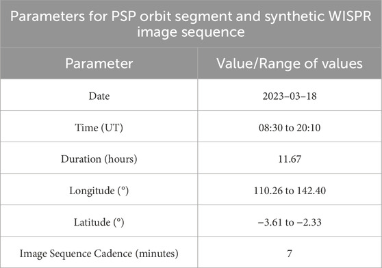
Table 1. These parameters indicate the physical parameters of the PSP trajectory used to generate the synthetic WISPR image sequence and the time cadence of the synthetic images.

Table 2

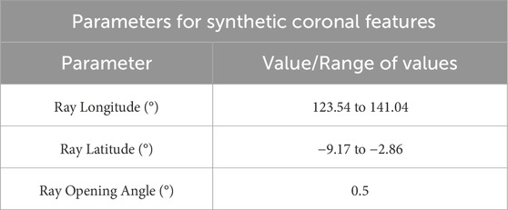
Table 2. The five synthetic, radial features used for this study are positioned at different locations, ranging in longitude and latitude between the given boundaries. Each ray is modeled as a cone, with a fixed angular width or opening angle of half a degree.

2.1 Lines of sight to cosmic radio sources

For typical coronal FR experiments, we select background sources (e.g., quasars, which are extremely luminous and compact active galactic nuclei) of linearly polarized radio emission with the principle goal of inferring the LOS component of the magnetic field of the intervening coronal plasma. In order to employ this method, we must select radio sources whose LOS traverse the WISPR FOV near perihelion so that the tomographic reconstructions can be of use to the FR observations. The tomography technique is of maximal utility near perihelion, when the spacecraft speed exceeds that of the corotating plasma.² The required observing geometry, therefore, restricts observations to a small patch of the sky when selecting sources.

For this demonstration of our WISPR-enhanced method, we have only performed the following geometric analysis for a single instant in time (18 March 2023 at 16:56 UT) which corresponds to the beginning of the FR observations and the approximate three-quarters-point of the PSP trajectory used for the tomography. While the celestial coordinates of our radio sources (i.e., J2000 Right Ascension, RA, and Declination, Dec) are fixed, the coordinates of the lines of sight to the sources change as a function of time, due to the Earth’s orbital motion around the Sun. For this initial study, we simplify the geometry involved by fixing the LOS to their positions at a single time-step.

Figure 1 illustrates the basic geometry, from two perspectives, for the FR observations coinciding with PSP Encounter 15, showing the position of each radio LOS in relation to the synthetic coronal striae (gray radial lines) and WISPR’s FOV (gray pyramid). We only show WISPR’s FOV at a single, arbitrary time-step. The five LOS to the observed radio sources appear in Figure 1 as colored lines. For each LOS ($1.5\mathrm{A}\mathrm{U}$ long), neither endpoint (Earth or the radio source itself) appears in the schematic. To help orient the reader, Earth is positioned to the lower right of each image, out of the frame.

Figure 1

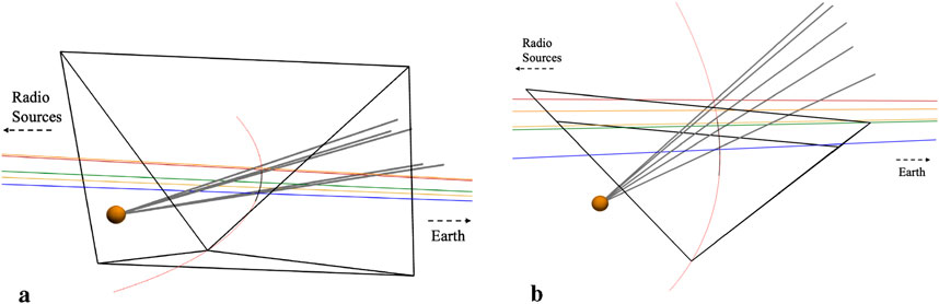
Figure 1. The two figures show different perspectives of the same scene: a schematic of WISPR looking out at radial features in the corona which intersect five lines of sight. The Sun is the orange sphere on the left; the five thick, gray radial spokes originating from the Sun represent the coronal rays; the five colored (red, orange, yellow, green, blue) lines represent the radio lines of sight from the background radio sources (off the image, to the left) to the Earth (off the image, to the right); the thin, curved red line indicates PSP’s actual trajectory during Encounter 15; the black section of the orbital path corresponds to the segment of the trajectory included in our synthetic image sequence; and the large, pyramidal shape–in thin, black lines–represents the WISPR field of view at perihelion for this encounter. (a) WISPR-LOS Coronal ray geometry. (b) Top-down view of geometry.

2.2 Synthetic coronal features

We generated five coronal rays with the following two important positional characteristics: they pierce WISPR’s FOV during the selected segment of the orbit and they intersect our radio LOS in the middle of the PSP trajectory used for this analysis. We included five radial features so that each radio LOS produces at least one intersection and so that we may work with several different intersection test cases. Knowing a priori that these features pierce the WISPR field and intersect our radio LOS, we can verify whether our tomographic reconstructions and subsequent analysis can recover those intersections.

As for the physical modeling of these features, we simply treat them as static, radial rays. WISPR routinely observes these striations in detail, but we do not yet understand their nature. Whether these striae constitute smaller-scale structure of, say, streamers and/or current/plasma sheets, or are instead distinct structures unto themselves, remains to be determined. As such, we utilize a physical model that makes few assumptions of the physical interpretation of such structures. In a future paper, we plan to develop more physically realistic models of these features and correspondingly model the FR signatures imposed.

Regarding the parameters of the features used for this demonstration, which are listed in Table 1, each feature takes the shape of a cone with a fixed opening angle of 0.5°. The width is therefore a function of radius alone. At a heliocentric distance of $1R_{\odot }$, one of such feature’s width is $\sim 10\mathrm{M}\mathrm{m}$, while at a radius of $10R_{\odot }$, its width is $\sim 100\mathrm{M}\mathrm{m}$. Note the narrow width of the rays compared to the length of the radio LOS; at a distance of $10R_{\odot }$, a feature’s $\sim 100\mathrm{M}\mathrm{m}$ width is a factor of 2,200 more narrow than the length of the radio LOS. As mentioned earlier, these modeled structures may represent fine-scale, filamentary structure within large-scale coronal structures. As posed in DeForest et al. (2018), whether these striae are individual structures, projection effects, or three-dimensional folds in the heliospheric current/plasma sheet remains an open question, but we will treat them as individual structures in this article. This assumption does not preclude these striae from being part of larger structures, e.g., a bundle of striae comprising a streamer, or a continuum of streamers forming a streamer belt. All of the features in this model possess the same central density, and since they have a fixed opening angle, their density drops off as $r^{-2}$ from the Sun.

Our forward model does not currently take into account the Thomson scattering angle, i.e., the angle between solar radial direction of the scattering site and the observer’s LOS to the scattering site. We intend to add the scattering angle into our forward model as a (near-term) future step. However, we do not expect the modeled radiance of the synthetic features to deviate significantly by adding a scattering angle parameter. In the integrand of the radiance equation, the term that depends on the scattering angle and the distance of the scattering site to the Thomson sphere is relatively flat over a large range of scattering angles (Howard and DeForest, 2012). While the real data reconstructions will likely still benefit from the addition of a Thomson scattering parameter, the synthetic data reconstructions would not change with the inclusion of a Thomson scattering parameter, because the basis elements and features in the image sequence are constructed identically. For more details on the forward model used to generate these features, please refer to Kenny et al. (2024).

2.3 PSP’s orbital trajectory and WISPR’s field of view

We use a segment of PSP’s Encounter 15 trajectory to make our synthetic WISPR image sequence, and we perform tomographic reconstructions of the synthetic coronal features’ positions in the resulting image sequence. The choice to include the true orbital geometry and radio LOS in our model is twofold. First, it better prepares us to employ this method to the actual FR observations in the future. Second, it provides the opportunity to further develop our translational tomography method, because the post-perihelion orbital geometry diverges from the ideal case (e.g., as discussed in Kenny et al., 2023; Kenny et al., 2024).

The parameters of both the PSP orbit segment and the synthetic image sequence corresponding to that orbit segment are summarized in Table 1.

2.3.1 PSP’s orbital trajectory

As we will expound upon in Section 3, our tomography relies on multiple vantage points of the coronal features whose three-dimensional structure we seek to reconstruct. The segment of the PSP orbit that we use to build an image sequence (with which we perform tomographic reconstructions) begins well before the FR observations begin because we require many images of the features well before PSP passes them in order to determine their positions. The duration of the orbit segment is $11.67\text{h}$, which corresponds to a change in heliographic longitude of about $32°$. PSP started out $14.9R_{\odot }$ from the Sun at the beginning of the orbit segment and moved out to $18.6R_{\odot }$ by the end of the $11.67\text{h}$ period. Figure 1 shows the actual orbital segment from the Encounter 15 trajectory (colored in red), with the portion used for the analysis (colored in black).

2.3.2 Modeling WISPR’s field of view during the perihelion 15 VLA observations

Before we can perform tomographic inversions on real WISPR data–during select encounters when the LOS to natural radio sources pierce the WISPR FOV–we must test our technique on synthetic data. Using the same code to generate synthetic data that Kenny et al. (2024) employ and describe therein, we generate a sequence of synthetic WISPR images of filamentary radial features (i.e., rays). We show a schematic of these features as gray spokes originating from the Sun and extending radially through the heliosphere in Figure 1. While the actual WISPR FOV is comprised of two separate, overlapping fields–an inner field and an outer field–our synthetic field is singular for simplicity.

Figure 2 shows nine images spanning the full image sequence to highlight the changes in apparent feature position and size throughout the image sequence. These nine images have a spacing of 77 min. The full image sequence is comprised of 101 images, which span 11.67 h and have a cadence of 7 min to best approximate the actual WISPR image cadence of 7.5 min during Encounter 15.

Figure 2

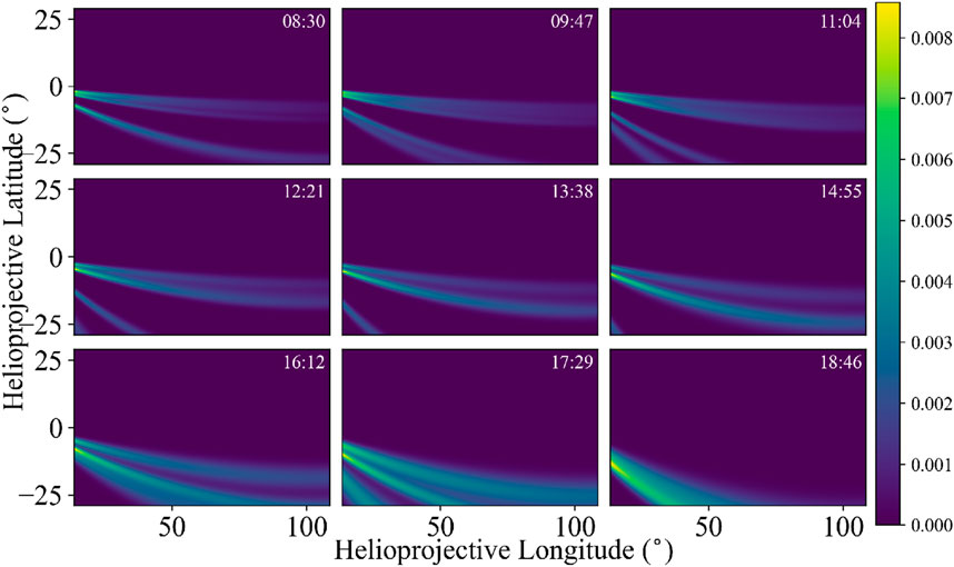
Figure 2. Nine synthetic images from our synthetic image sequence span the full 11.67-h dataset. In order to highlight the apparent motion of the features through the FOV, every 11th image is shown. The axes are longitude and latitude in helioprojective coordinates. Time moves from left to right and top row to bottom row. At the top right corner of each image, the timestamp (in UT) is displayed. The quasi-static coronal features (corresponding to the gray radial striae in Figure 1) appear to move through the FOV as the spacecraft approaches and passes them in its orbital motion. In later images (e.g., the bottom row), all coronal features appear to exit the image at the bottom left because PSP’s trajectory takes it above them. The colorbar to the right of the images indicates the brightness of the radial features in arbitrary units.

The radial features appearing in the images of Figure 2 have different angular locations, spanning a heliographic longitudinal range of 17.5° and a heliographic latitudinal range of 6.3°. PSP therefore flies past them at different times, and our synthetic WISPR images capture ever-changing viewpoints of these quasi-static features³.

Next, we will describe how we reconstruct the positions of these features and localize their intersections with the radio LOS.

3 Methods

The high-level methodology is to use tomographic reconstructions of WISPR image sequences (as developed in Kenny et al., 2023; Kenny et al., 2024) to determine (1) the three-dimensional positions of local, radial density enhancements that appear in the WISPR FOV as striations within large-scale density structures, and (2) the intersections of these features with LOS to radio sources for coronal FR observations. The primary focus of this article is the second goal: localizing the intersections of the features with the radio LOS. It is worth noting that only the density structures appearing in WISPR’s FOV, sufficiently close to perihelion, are candidates for tomographic reconstruction; accordingly, our tomography will not constrain the positions of density enhancements along the radio LOS that fall outside the WISPR FOV.

For the purpose of this present work, we use the LOS to the five cosmic radio sources that we observed on 18 March 2023 – the day after PSP Perihelion 15. While this method will be applicable to any FR observations (or, more generally, any observations along a LOS or trace through the WISPR FOV), for this proof-of-concept demonstration we used the actual LOS to the radio galaxies observed during Encounter 15, as well as PSP’s true orbital trajectory during these observations in creating the synthetic image sequence for this analysis.

Our observations during Perihelion 15 correspond to the first (of three total) PSP/WISPR-coordinated FR observations and will be the first set of FR observations that we analyze in a future article. As such, the analysis present in this article will serve as a stepping stone to the forthcoming FR analysis with application of the tomography to the actual WISPR data. The WISPR-LOS geometry for these observations also introduces a unique opportunity: to further develop our tomography method, making it more robust for different observing geometries. These observations were made post-perihelion, i.e., the orbital trajectory of PSP is monotonically outbound. Kenny et al. (2023) and Kenny et al. (2024) only consider the ideal orbital geometry, with the trajectory of PSP centered on the perihelion itself, for tomographic reconstruction of coronal features. The orbital geometry required by the LOS direction from our radio sources to the Earth relative to PSP’s position and WISPR’s field of view (e.g., Figure 1) is non-ideal because PSP is constantly getting further away from the Sun. The primary consequence of this is the coronal features observed are getting progressively less dense and, therefore, less bright. This non-ideal geometry, thus, makes the three-dimensional reconstruction with translational tomography much more challenging.

3.1 Performing a tomographic reconstruction on the synthetic image sequence

In order to determine where along the radio LOS density enhancements exist, we must first determine their positions in three-dimensional space. This tomographic inversion technique in principle can reconstruct the three-dimensional plasma density distribution in the vicinity of the spacecraft with boundaries imposed by the field of view. However, in this article, we reconstruct a two-dimensional map because our basis set uses a single line of sight (rather than the full field of view) from each image. Furthermore, while the values in our tomographic maps are proportional to the local densities, we have not determined a method to calibrate the maps in order to infer densities from them. Herein, we focus on the inferred positions of local density enhancements rather than the numeric densities.

Our ability to extract local density information hinges on WISPR capturing many unique viewpoints of these features, which PSP’s rapid translational motion past and through these features affords us. We must also be able to model these unique perspective changes in the WISPR FOV in order to build a basis set, i.e., a set of functions that are used to represent operators, with which we can reconstruct local plasma density.

These reconstructions work by performing a matrix inversion, effectively changing the basis of the dataset from image coordinates (i.e., time-dependent angles defined by PSP’s trajectory in relation to points along the coronal features) to tomographic/parametric coordinates (i.e., static positions of these coronal density features in space). Please see Kenny et al. (2023) and Kenny et al. (2024) for details on the mathematical operations of the inversions.

Up to this point, the procedure for performing a tomographic reconstruction of radial features has consisted of the following steps:

1. Make a single, composite image for a dataset called the ‘T-Map’ which is a time-angle data product⁴, an example of which appears as Figure 3.

2. Construct a (partial) basis set of time-angle curves⁵ to represent all possible features appearing in the synthetic image sequence (and, therefore, in the T-Map).

3. Take the dot product of each element of this basis set (i.e., each basis vector, an image with the same dimensions as the T-Map) with the T-Map.

4. Populate a new image–called a ‘tomogram’ – whose axes are the tomographic coordinates–with the values of each dot product operation. The numeric value at each pixel is proportional to the intrinsic brightness of the feature, which is proportional to the local density.

Figure 3

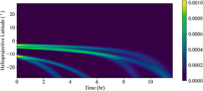
Figure 3. This time-angle image is called a “T-Map” and represents the change in transverse angle, with respect to PSP’s orbital trajectory, of a particular point of plasma along each feature throughout the course of the image sequence. The T-Map is a composition of columns–one column per image–such that the entire image sequence is captured in a single image. In the T-Map shown here, five curves correspond to five (synthetic) radial striae that appear in our synthetic WISPR field of view during the 11.67-h image sequence. To retrieve the parameters of the curves in the T-Maps, and thus the positions of the features they represent, we must take the dot product of the basis of image curves with the T-Map. The colorbar on the right of the image indicates the brightness of the features in arbitrary units.

Expanding on the first step in the enumerated list above, a T-Map is a time-angle image that represents the temporal change in the transverse angle of (a particular point of plasma along) each feature throughout the image sequence. Each image in our sequence contributes a single column to the T-Map. Figure 3 shows the change in apparent latitude of the five (synthetic) radial striae throughout the duration of the image sequence. To retrieve the parameters (and thus the three-dimensional positions) of the radial features, we must take the dot product of the basis of image curves with the T-Map. Each of these dot products corresponds to a particular pair of angular coordinates, and the tomogram (of which Figure 4 is an example) shows us the value of each dot product.

Figure 4

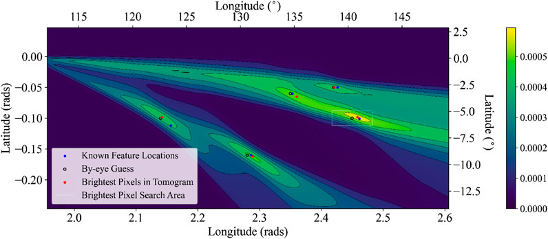
Figure 4. The tomogram is the primary product of the translational tomography calculation and visually represents the dot product operations between each basis vector and the T-Map (e.g., Figure 3). The tomogram provides the coronal feature coordinates in heliocentric longitude and latitude pairs. The brightest regions indicate the parameters of the features in the image sequence but are stretched out due to the non-orthogonality of the basis set. The known parameters (blue points), initial guesses of the brightest pixels (black circles), and true location of the brightest pixels (red stars) are plotted on top of the image. These three sets of coordinates all lie within the brightest clusters of pixels on the image and within the six-by-four pixel neighborhood of the initial guess coordinates. The single dashed-line rectangle centered on the initial guess, enclosing the bright pixels at the largest longitudes, demonstrates the bounds of the search vicinity for that particular feature and represents the search area used for all other features. The colorbar on the right of the image indicates the brightness of the features in arbitrary units, and the contours on the tomogram delineate the colorbar levels.

Locations in the tomogram where the dot products attain a local maximum theoretically indicate a given feature’s parameters and, thus, enable us to determine the three-dimensional positions of the radial rays. For a detailed description of this process, please see Kenny et al. (2023) and Kenny et al. (2024).

As we discuss at length in both of the foundational papers on translational tomography, the tomographic reconstructions do not recover a single pair of parameters for each feature. The non-orthogonality of the basis vectors results in many different basis vectors (with different assigned parameters) all yielding comparable dot products. Therefore, it can be difficult to determine which pair of parameters describes each feature. Other factors that further complicate the extraction of feature parameters include: the orbital path of PSP, the feature’s distance away from the PSP orbital plane, the feature’s brightness (i.e., density relative to the ambient solar wind), and the number and cadence of images available.

Once we have a tomogram, the number of local maxima should equal the number of features in the image sequence. We search for a set of the brightest pixels within each local maximum on the map. The brightest pixels on the tomogram correspond to the largest dot products (of the basis elements and the T-Map), and each dot product corresponds to a pair parameters for the features in the dataset. Inspecting the tomogram, we supply initial guesses and search for the brightest pixel within a field on the image that is large enough to cover the cluster of bright pixels (relative to the surrounding part of the image) and small enough to remain in the local maximum region. For each guess, when a brighter pixel has been identified within the specified search field, the parameters are updated until the search field has been exhausted. Once we have the parameters–heliocentric longitude and latitude⁶ – we can solve for their intersections in three-dimensional space with the radio LOS.

3.2 Determining the intersections between the lines of sight to radio sources and the synthetic coronal features

With three-dimensional coordinates recovered by the tomographic inversions, we can determine where along the radio LOS these radial density features lie. We also calculate the physical extents of those intersections, using the model parameters for the coronal features as described in 2.2. We discretize each radio LOS so that we may calculate the distance between the LOS and each feature for a finite set of points along the LOS. We use 10,000 points for each LOS, resulting in a spatial resolution of $1.5\times 10^{-4}\mathrm{A}\mathrm{U}$ (or $22.4\mathrm{M}\mathrm{m}$).

As Figure 5a shows, at each point we determine: the closest distance to the analytic line representing the central axis of the $i^{th}$ coronal density feature, $d_i$, and the coordinates on the feature’s central axis that correspond to this closest distance. If the distance $d_i$ falls within the local radius $(w(r))$ of the feature–using model parameters for the radial, conical rays of fixed opening angle–then we infer an intersection between the feature and the radio LOS. Keeping track of each discrete point that satisfies this intersection criterion, we can thus infer the path length of each intersection along the radio LOS calculating the length between the endpoints for each set of intersection points. It is important to note that the intersection path length calculation described here relies on model parameters for the rays, rather than recovering physical widths from the tomography.

Figure 5

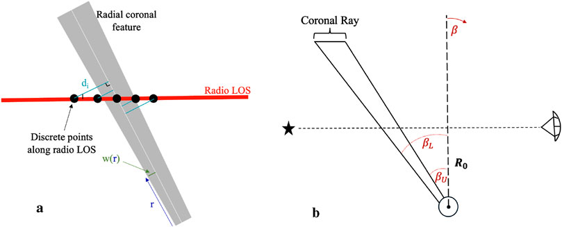
Figure 5. These two schematic diagrams show how we solve for intersections between coronal features and radio LOS (a) and how we parameterize a feature’s location along a LOS (b). (a) Intersection Geometry Schematic: In order to solve for an intersection between a radio LOS (red line) and the ith radial coronal feature (gray cone), we discretize the continuous line of sight into 10,000 points. At each point, we calculate the distance di to the central axis of the coronal feature. If di is less than the local width of the cone w(r), then the line of sight and coronal feature are intersecting. In this illustration, only two LOS points meet the criterion that di ≤ w(r). (b) FR ß Parameterization: A cartoon exemplifying the parameter ẞ that encapsulates where a coronal feature intersects a LOS from a radio source (left) to a telescope on Earth (right). The shortest distance between the LOS and the Sun center is Ro. The angle ẞ is measured from the perpendicular line between the Sun center and the radio line of sight. The upper and lower values, Bu and BL respectively, indicate the boundaries of the coronal feature along the LOS. This figure is comparable to the fundamental modeling geometry used in FR observations (e.g. Fig. 1 in Kooi et al., 2022).

Finally, we can parameterize these intersection locations and extents along the radio LOS with an angle, $\beta$, which denotes the angle from the perpendicular line that connects the center of the Sun to a radio LOS at which a coronal feature-LOS crossing occurs. The angle $\beta$ indicates where along the radio LOS a point lies, replacing the distance $\vec{s}$ along the LOS (from Equation 1). This parameterization is commonplace in FR modeling and experiments, and since the results of these reconstructions will be used to improve the sensitivity of future FR measurements, we give our results in this form. Figure 5b illustrates the $\beta$ parameterization of the coronal feature-LOS geometry, indicating the upper and lower boundaries of an intersection between a coronal ray and a radio LOS (as ${\beta }_U$ and ${\beta }_L$ respectively).

4 Results

4.1 Tomography

The primary output of our tomographic inversion is the “tomogram” in Figure 4. A tomogram is an image whose dimensions are the tomographic parameters, in this case heliocentric longitude and latitude, and whose numeric value at each pixel scales with the brightness at the respective coordinate pair. We arrive at this image by taking the dot product of each basis vector with the T-Map. Each dot product (which maps to a particular basis element with unique (lon, lat) coordinates) is assigned to those coordinates on the tomogram. Therefore, the brightest pixels on the tomogram indicate the (lon, lat) pairs that best match the features in the T-Map. In Section 5 we will discuss why the distribution and brightness of pixels may deviate from the simple explanation above.

Returning to the tomogram–Figure 4 – we see that the ground-truth feature locations (as indicated by blue dots) fall within the five brightest clusters of pixels. However, it is clear that the brightest pixels fill extended, asymmetric regions around the true feature locations as opposed to a single bright pixel, or even a few pixels. Furthermore, the ground-truth feature locations do not lie at the centers of all the bright pixel clusters, as we might intuitively expect. It is not obvious, without prior knowledge, what the feature parameters are by inspecting the tomogram. Therefore, we search for the brightest pixel within a specified vicinity of a guess for each feature.

Figure 4 shows the pixels corresponding to not only the known feature locations (again as blue dots) but also the by-eye guesses (as unfilled, black circles) and the brightest pixels (as red stars). Intensity contours demarcate the different levels indicated on the colorbar. Additionally, a representative search-area box at (lon, lat) = (2.35, −0.06) is shown in Figure 4 as a white, dashed-line rectangle. For this particular analysis, we searched within a rectangle 12 pixels wide and eight pixels tall centered on the by-eye guess for each feature; the higher resolution in latitude causes the rectangle to appear more stretched out in width (i.e., to have a larger aspect ratio).

Additionally, Table 3 provides the coordinates of the by-eye guesses, ground-truth coordinates, and location of the true brightest pixels. The brightest pixels are not the same pixels as those corresponding to the actual feature parameters, which we will discuss in the following section. However, there is not a clear pattern in the relative locations of the brightest pixels and their ground-truth counterparts. Despite the challenges in interpreting the tomogram, we must use a method to extract feature locations from the image since, in reality, we will not know the ground-truth locations. Here we use the angular coordinates corresponding to the brightest pixels as the reconstructed parameters.

Table 3

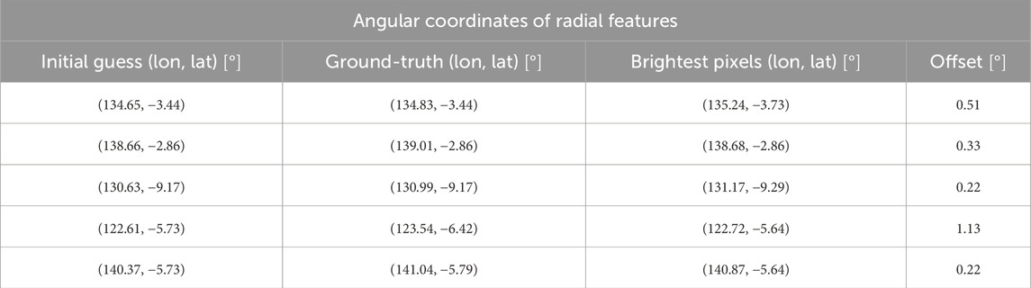
Table 3. For each feature, we provide the angular coordinates of the guess (by visual inspection of the tomogram), the known parameters, and the brightest pixel determined by a search within the vicinity of the guess (e.g., see the boxes in Figure 4). The final column gives the net angular offset between the known feature parameters and the tomographically recovered brightest pixels.

4.2 Intersections between coronal features and lines of sight

Assigning the coordinates of the brightest pixels in the tomogram to radial rays in the corona, we can then solve for the intersections of these rays with our radio LOS. Section 3 describes the particular conditions that constitute an intersection. Each of the five brightest pixels identified in the tomogram (indicated as red stars in Figure 4) results in an intersection with one or two radio LOS. These inferred intersections lie near the true intersections. The results of the geometric computations yield the intersection boundaries (i.e., the starting points and endpoints of the section of each LOS contained within the coronal feature) and the extent along the LOS of the intersections using the model parameters. We parameterize these quantities in terms of the angle $\beta$ (as illustrated in Figure 5b). Figure 6a illustrates the geometry of the intersections between these coronal features and the radio LOS from the perspective of the LOS-Sun-Earth plane that is typically used in coronal FR modeling (and shown in Figures 5b, 6a).

Figure 6

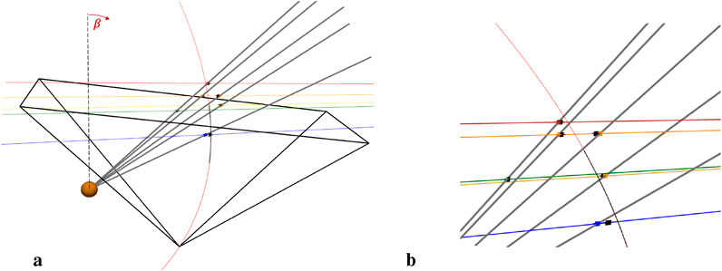
Figure 6. Most of the elements appearing in these figures also appear in Figure 1, but we have added the ground-truth intersection points between the synthetic rays and the radio LOS (represented by colored strips that correspond to the line of sight that the ray intersects), as well as tomographically recovered intersections (represented by black strips along the lines of sight). Finally, we include a radial, dashed line in (a)–extending from the Sun center approximately perpendicular to the radio lines of sight; we measure the angle $\beta$ from this line and thus show in this schematic how we will determine the $\beta$ values for the given intersections. (a) Top-down view of (true and inferred) intersections between coronal rays and radio LOS. (b) Zoomed-in view of true and inferred ray-LOS intersections.

We can identify six intersections with the radio LOS: colored strips for intersections with the true locations of the synthetic rays and black strips for the intersections with the tomographically-recovered ray locations. While the two sets of intersections appear approximately overlapping for the red LOS, it is clear that those along the blue LOS are spatially separated, especially in Figure 6b which is a zoomed-in view of the intersections appearing in Figure 6a. Referring back to Figure 4, the feature for which the brightest pixel deviated most from the ground-truth pixel was that at the smallest longitude (with (lon, lat) coordinates of ($123.54°$, $-6.42°$)). Having the smallest longitude of all the features, this feature appeared in the fewest number of images, resulting in a less pronounced peak at and around the ground-truth parameters on the tomogram, and thus a substantially larger error in $\beta$ (seen in Table 4).

Table 4

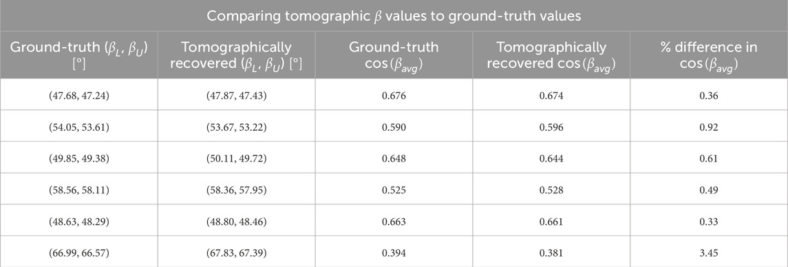
Table 4. In this table, the two left-most columns provide the lower and upper bounds on the coronal rays with respect to the radio lines of sight they intersect–for both the ground-truth feature coordinates and the coordinates calculated using the translational tomography. The third and fourth columns display the cosine of the average intersection angle, $cos({\beta }_{\mathit{avg}})$, and the final column shows how close the tomography results come to the actual values.

Because our tomography reconstructions do not recover the exact angular coordinates of the features, the lengths of the intersections between the reconstructed rays and radio LOS differ from those between the actual rays and radio LOS. Although Figure 6 does not make obvious the physical extent of these intersections, the finite widths of the rays (which we modeled as cones with fixed opening angles) result in intersections of finite widths. Therefore, the location at which the intersection occurs determines the length of the intersection. Furthermore, the relative angle between the radio LOS and a given ray also impacts the extent to which a coronal feature intersects a radio LOS. Table 4 gives the upper and lower bounds of each intersection (${\beta }_U$ and ${\beta }_L$), for both the ground-truth synthetic rays and the tomographically reconstructed rays, and the cosine of the average values. Since the factor $cos(\beta )$ appears in analytic models of FR, it is useful to compare this factor between the tomography and ground-truth values. The final column of Table 4 reports the percent error of the recovered $cos(\beta )$ values from the ground-truth values. Five of the six values differ by less than a percentage point, with the exception of a few-percentage-point-difference for the remaining value. In future analyses we will estimate uncertainties in extracting feature coordinates from our tomography and propagate that uncertainty in the calculation of $\beta$ and intersection lengths.

5 Discussion

In this section, we discuss the two primary areas of the project: tomography and modeling. We review the insights we have taken from this demonstration of a new method, the challenges of the present methodology, and the next steps that will improve the technique for future application to real WISPR data in order to enhance radio FR studies of the coronal magnetic field.

5.1 Tomography

Our tomographic maps, called tomograms, are two-dimensional maps that indicate local density enhancements around the spacecraft. While the numeric pixel value at each pair of heliocentric coordinates scales with the intrinsic brightness, and thus the density, at those coordinates, we have not calibrated the inversions to recover numeric plasma density values. Furthermore, this article is primarily concerned with locating the density enhancements along lines of sight to radio sources. Nonetheless it is nontrivial to infer the positions of ray-like density enhancements.

The non-orthogonality inherent to this inversion approach, which we discuss at length in Kenny et al. (2023) and Kenny et al. (2024), means that the dot product of any two distinct basis vectors may be nonzero. Consequently, each feature in a dataset will activate several different basis elements. Even in the case of these synthetic inversions, where the basis elements are morphologically identical to the features themselves, we cannot recover a unique solution. Furthermore, the particular orbital geometry that we use for this demonstration presents additional challenges. The orbital segment used (08:30 UT - 20:10 UT on 18 March 2023) occurred exclusively after perihelion (20:30 UT on 17 March 2023) in Encounter 15. Consequently, the synthetic images and the basis elements capture plasma that is increasingly farther from the Sun, resulting in lower signal-to-noise in the images.

In the T-Map, Figure 3, this effect is particularly clear in the curves that exit the FOV at the later times; these curves widen and become more diffuse towards the end of the image sequence. In the tomogram, the post-perihelion orbital segment broadens the cluster of brighter pixels around each feature’s true parameters and introduces asymmetry to the quasi-elliptical cluster. It is especially problematic when two features are at very similar viewing angles, e.g., the pair of features at (lon, lat) coordinates of (134.83° − 3.44°) and (141.04° − 5.79°) in Figure 4. The associated clusters of pixels for these two features overlap/merge; resolving them into two separate features becomes very challenging. There is more work to be done to quantify how orbital geometry and other parameters introduce additional ambiguities to the inversion results. Furthermore, adding a scattering angle parameter to the model may help to disambiguate distinct features.

An area we intend to explore is the use of multiple tomograms to improve the amount of information we are utilizing for our inversions. As discussed in Kenny et al. (2024), it is possible to create a unique set of basis vectors for each elongation angle in the field of view. The resulting set of tomograms would likewise have unique distributions of brightness, and the combination of these different reconstructions should be able to better constrain the parameters for each feature. We may even be able to simply cross-correlate the tomograms in the set. Minimizing the sizes of bright pixel clusters on the tomogram mitigates the extent to which a person must interpret the tomogram. Once we have further developed the translational tomography method to incorporate these changes, we can implement a new algorithm that automatically locates the local maxima and, thus, the locations of coronal features without the need for human interpretation.

5.2 Modeling

We now discuss the modeling portion of this project in the context of future studies that will build off this work. In Section 2, we modeled: five lines of sight through the WISPR field, using the coordinates of the actual radio sources that we observed during PSP Encounter 15; five synthetic coronal rays that were generated specifically to intersect the radio LOS; and the WISPR FOV for an approximately 12 h PSP orbital trajectory.

Using the LOS to the radio galaxies that we observed during Encounter 15 for this demonstration gives us a head start on the forthcoming FR analysis for those observations. However, we will relax the constraint that the LOS are fixed in time, allowing the radio LOS to move as a consequence of Earth’s orbital motion. In typical coronal FR observations, the impact parameter ($R_0$ in Figure 5b, the distance between the Sun and the proximate point along the LOS) changes by $\sim 0.5{\mathrm{R}}_{\odot }$ over the course of six to 8 hours of observing a background radio galaxy. This modification will make the reconstructed intersections more accurate, providing the detailed localization and density variation information necessary to ensure a more sensitive magnetic field estimate from the FR measurements.

The next area we explore includes the synthetic features themselves. We modeled five radial rays that appeared in WISPR’s FOV and that intersected with the radio lines of sight fixed in their positions at the beginning of the radio observations (halfway through the PSP orbital segment). Similar to the radio LOS, we employed a simplifying approximation for the synthetic rays used in this present work: we keep them fixed in an inertial reference frame. It has been found that large-scale radial structures in the corona, of which these rays may be a part, do not appear to evolve on timescales of $\sim$10 h (e.g., Fisher and Guhathakurta, 1995), which is longer than most individual FR observational campaigns with the VLA. Furthermore, our tomography is only applicable during periods of super-rotation, i.e., when PSP is traveling faster than the co-rotating plasma. However, we intend to develop more realistic models of these features, namely, modeling these rays as streamlines (or substructure of streamlines) along which radially out-flowing plasma travels. These Archimedean spirals will approximate radial rays at small heliocentric distances but will take on appreciable azimuthal components further out. This consideration will be particularly important for reconstructing features in WISPR’s outer field of view, which images features at much larger radial distances than the inner detector. Moreover, any plasma that PSP samples in situ appears in the outer detector of WISPR, before PSP reaches it; therefore, the outer FOV inversions have the unique capacity to connect what we see in WISPR data to other PSP measurements. Even when we advance from synthetic to real WISPR data, we will still utilize the synthetic basis elements in order to perform matrix inversions of the image sequences, and thus it will be remain necessary to improve the physical modeling of the features.

The next modeling element we will address is the orbital geometry. As we have touched on already, the particular orbital path we use for this demonstration poses challenges to the tomographic inversions. Because the approximately 12 h period begins on the day after PSP’s closest approach to the Sun in Orbit 15, the spacecraft moves increasingly further away from the Sun throughout the orbital segment. The primary effect of PSP moving away from the Sun is that WISPR images features correspondingly further from the Sun. For example, at perihelion of Encounter 15, PSP dipped down to a height of $13.3{\mathrm{R}}_{\odot }$, and the WISPR FOV spanned $3.1-24.2{\mathrm{R}}_{\odot }$ (at a latitude of $0°$). Meanwhile, the FOV ranges imaged by WISPR during the orbital segment selected for this demonstration were $3.4-27.2{\mathrm{R}}_{\odot }$ (at a radial distance of $14.9{\mathrm{R}}_{\odot }$) and $4.3-33.8{\mathrm{R}}_{\odot }$ (at a radial distance of $18.6{\mathrm{R}}_{\odot }$). While we could have chosen to use a more favorable orbital path for the demonstration of this new method, it was useful to work with the actual segment that we will use in the analysis of the FR observations during Encounter 15, to engage with the unique uncertainties introduced by orbital geometry parameters, and to develop strategies to mitigate these issues moving forward.

Finally, though it is not strictly a matter of modeling, we calculated the intersection path length using the model parameters of the rays. A near-term improvement would be to estimate the widths of the recovered features from their apparent sizes in the images. Assumptions about the form of the features (i.e., cones of fixed angular width) would still be necessary. Regardless of the method utilized, a more rigorous treatment of uncertainties–from the inference of feature positions from the tomogram to the estimation of the intersection path length–is necessary for future analyses.

6 Conclusion

In this article, we have presented a new application of an in-development tomographic technique: using WISPR translational tomography to 1) extract information on density variations in the vicinity of the spacecraft, and 2) determine the intersections of the recovered features with LOS to radio galaxies for coronal Faraday rotation (FR) studies. FR-derived magnetic field estimates are subject to the errors in plasma density estimates, as FR depends on the product of electron plasma density and magnetic field, both of which vary along the LOS. Current methods to infer plasma density only return integrated quantities (i.e., a sum over the whole LOS) rather than any information about variations along the LOS. This reality is troubling; the most important parameter to estimate in the FR equation is where different plasma structures intersect the LOS.

To properly calibrate FR data and account for the plasma density’s contribution, more reliable modeling of the electron density, integrated along the LOS to the radio source, is necessary. In this article we have laid out a method to infer plasma density enhancements along a LOS that traverses the WISPR FOV. Future papers will focus on quantifying the extent to which these tomographic reconstructions impact the modeled FR signal–utilizing different models of density structures, and on calibrating the tomographic reconstructions such that we can make electron density estimates. In terms of the impacts on FR experiments, our tomographic reconstructions will enable more accurate estimates of the neutral line crossing location(s) as well as tighter constraints on parameters of electron density models, such as the streamer belt width and boundaries between under- and overdense regions.

As a proof-of-concept demonstration and a description of a method used to calibrate plasma measurements, this project utilized an image sequence of synthetic coronal density structures, along with a real PSP orbital trajectory during a set of FR observations and the real LOS to the observed radio galaxies corresponding to those FR observations. The combination of modeled and real elements of our system strikes a balance between building a tractable problem–in order to develop a new method–and introducing the oft-unforeseen challenges of the physical world. Furthermore, the use of the actual radio LOS and PSP trajectory better prepares us to implement this method to the corresponding FR observations, with real WISPR data inversions.

In this article, we have sought to describe a method of inferring plasma density enhancements along lines of sight that traverse the WISPR FOV. We have divided the method into two components: tomographic reconstructions of the density-enhanced rays and localization of the rays’ intersections with LOS to background radio sources. The first component, the tomographic reconstructions, leverages characteristic perspective changes (in WISPR’s FOV) of radial striae in the vicinity of PSP in order to reconstruct density information around the spacecraft. While this tomographic technique has been tested on synthetic data before, the test case used for this methodological demonstration contended with non-ideal orbital parameters and closely spaced features. This departure from ideal geometry has served as a stepping stone from synthetic data to real data inversions. Although refinement of the technique is ongoing, we are now in the process of inverting real WISPR image sequences.

Seeing the effects of non-ideal geometry on the tomographic reconstructions, we discussed ideas to improve the inversions. One idea we presented was to generate multiple sets of basis elements–using different slices of the images (i.e., different viewing angles) – to perform our inversions. Utilizing multiple basis sets results in multiple, unique tomograms. Another idea is to use the entire image sequence rather than a single slice of pixels from each image. We are presently following this latter approach in reconstructing real data.

The second component of this project is to take the tomographically recovered angular positions of the features, assume they are radial cones, and determine their intersections with the radio LOS. We parameterize the intersections using the $\beta$ parameter typically used to model FR observations. Our results are encouraging: we find the same number of intersections between tomographically recovered features and radio LOS as we do between the ground-truth features and the radio LOS, though the intersections differ in position and extent. This difference, however, is minor, as demonstrated in Table 4. While we have determined several areas in which we can refine this technique before it is truly operational, this first effort to localize LOS plasma density variations is promising for the advancement of FR studies and, more broadly, remote-sensing studies of propagation effects due to the solar wind. Finally, there are certainly other applications of this work to derive information on the variations of density along a LOS or trace through the WISPR FOV, such as determination of coronal plasma structures intersecting comet paths.

Data availability statement

The raw data supporting the conclusions of this article will be made available by the authors, without undue reservation.

Author contributions

KK: Conceptualization, Formal Analysis, Investigation, Methodology, Software, Writing – original draft, Writing – review and editing. JK: Conceptualization, Formal Analysis, Methodology, Supervision, Writing – review and editing. SVK: Formal Analysis, Supervision, Visualization, Writing – review and editing, Software. CD: Supervision, Writing – review and editing.

Funding

The author(s) declare that financial support was received for the research and/or publication of this article. KK, CD, and SVK acknowledge support for this work by the NASA Parker Solar Probe office for the WISPR program, under contract No. NNG11EK11I to NRL and subcontract No. N00173-20-C-2002 to Southwest Research Institute. KK is also supported by NASA FINESST grant No. 80NSSC24K1859. The work of KK on the foundational tomography method was also supported by the National Science Foundation Graduate Research Fellowship under Grant DGE 1650115. Basic research at the U.S. Naval Research Laboratory (NRL) is supported by 6.1 Base funding.

Acknowledgments

We thank the entire WISPR team–Mark Linton and Roger B. Scott in particular–for fruitful discussions and ongoing support. Parker Solar Probe was designed, built, and is now operated by the Johns Hopkins Applied Physics Laboratory as part of NASA’s Living with a Star (LWS) program (contract NNN06AA01C). Support from the LWS management and technical team has played a critical role in the success of the Parker Solar Probe mission. The Wide-Field Imager for Parker Solar Probe (WISPR) instrument was designed, built, and is now operated by the US Naval Research Laboratory in collaboration with Johns Hopkins University/Applied Physics Laboratory; California Institute of Technology/Jet Propulsion Laboratory; University of Gottingen, Germany; Centre Spatiale de Liege, Belgium; and University of Toulouse/Research Institute in Astrophysics and Planetology.

Conflict of interest

The authors declare that the research was conducted in the absence of any commercial or financial relationships that could be construed as a potential conflict of interest.

Generative AI statement

The author(s) declare that no Generative AI was used in the creation of this manuscript.

Publisher’s note

All claims expressed in this article are solely those of the authors and do not necessarily represent those of their affiliated organizations, or those of the publisher, the editors and the reviewers. Any product that may be evaluated in this article, or claim that may be made by its manufacturer, is not guaranteed or endorsed by the publisher.

Footnotes

¹The Zeeman effect is when an external magnetic field splits spectral lines.

²In a period of super-rotation, we can treat the coronal rays as quasi-static, which simplifies the tomographic method.

³The assumption that the features are fixed in an inertial frame is a simplification, as we believe these features are actually co-rotating with the Sun.

⁴A T-Map shows how the helioprojective latitudinal angle to features changes as a function of time across the entire image sequence; we build it by stacking up one column of pixels from each image side by side.

⁵We generate the basis elements using the same set of pixel columns as for the T-Map.

⁶under the assumption that the features are radial.

References

Athay, R. G., and Beckers, J. M. (1976). The solar chromosphere and corona: quiet sun. Phys. Today 29, 74–76. ((Dordrecht: Reidel)). doi:10.1063/1.3024520

CrossRef Full Text | Google Scholar

Brueckner, G., Howard, R., Koomen, M., Korendyke, C., Michels, D., Moses, J., et al. (1995). “The large angle spectroscopic coronagraph (lasco),” in The SOHO mission (Springer), 357–402.

CrossRef Full Text | Google Scholar

DeForest, C., Howard, R., Velli, M., Viall, N., and Vourlidas, A. (2018). The highly structured outer solar corona. Astrophysical J. 862, 18. doi:10.3847/1538-4357/aac8e3

CrossRef Full Text | Google Scholar

Fisher, R., and Guhathakurta, M. (1995). Physical properties of polar coronal rays and holes as observed with the spartan 201-01 coronagraph. Astrophysical J. 447, L139. doi:10.1086/309582

CrossRef Full Text | Google Scholar

Fox, N., Velli, M., Bale, S., Decker, R., Driesman, A., Howard, R., et al. (2016). The solar probe plus mission: humanity’s first visit to our star. Space Sci. Rev. 204, 7–48. doi:10.1007/s11214-015-0211-6

CrossRef Full Text | Google Scholar

Golub, L., and Pasachoff, J. M. (2010). The solar corona. Cambridge University Press.

Google Scholar

Hayes, A., Vourlidas, A., and Howard, R. (2001). Deriving the electron density of the solar corona from the inversion of total brightness measurements. Astrophysical J. 548, 1081–1086. doi:10.1086/319029

CrossRef Full Text | Google Scholar

Howard, R. A., Stenborg, G., Vourlidas, A., Gallagher, B. M., Linton, M. G., Hess, P., et al. (2022). Overview of the remote sensing observations from psp solar encounter 10 with perihelion at 13.3 r. Astrophysical J. 936, 43. doi:10.3847/1538-4357/ac7ff5

CrossRef Full Text | Google Scholar

Howard, R. A., Vourlidas, A., Colaninno, R. C., Korendyke, C. M., Plunkett, S. P., Carter, M. T., et al. (2020). The solar orbiter heliospheric imager (SoloHI), Astron. Astrophys., Sol. Orbiter Heliospheric Imager (SoloHI). 642, A13. doi:10.1051/0004-6361/201935202

CrossRef Full Text | Google Scholar

Howard, T., and DeForest, C. (2012). The thomson surface. i. reality and myth. Astrophysical J. 752, 130. doi:10.1088/0004-637x/752/2/130

CrossRef Full Text | Google Scholar

Ingleby, L. D., Spangler, S. R., and Whiting, C. A. (2007). Probing the large-scale plasma structure of the solar corona with faraday rotation measurements. Astrophysical J. 668, 520–532. doi:10.1086/521140

CrossRef Full Text | Google Scholar

Jackson, B. V., Buffington, A., Cota, L., Odstrcil, D., Bisi, M. M., Fallows, R., et al. (2020). Iterative tomography: a key to providing time-dependent 3-d reconstructions of the inner heliosphere and the unification of space weather forecasting techniques. Front. Astronomy Space Sci. 7. doi:10.3389/fspas.2020.568429

CrossRef Full Text | Google Scholar

Jackson, B. V., and Hick, P. P. (2004). “Three-dimensional tomography of interplanetary disturbances,” in Solar and space weather radiophysics: current status and future developments (Springer), 355–386.

Google Scholar

Jensen, E., Frazin, R., Heiles, C., Lamy, P., Llebaria, A., Anderson, J., et al. (2016). The comparison of total electron content between radio and thompson scattering. Sol. Phys. 291, 465–485. doi:10.1007/s11207-015-0834-5

CrossRef Full Text | Google Scholar

Kenny, K., DeForest, C., Van Kooten, S., and Liewer, P. (2024). Translational tomography with the wide-field imager for parker solar probe (wispr). ii. refinements to the method. Astrophysical J. 975, 283. doi:10.3847/1538-4357/ad808c

CrossRef Full Text | Google Scholar

Kenny, K. N., DeForest, C. E., West, M. J., and Liewer, P. C. (2023). Translational tomography with the wide-field imager for parker solar probe (WISPR). I. Theoretical basis and initial modeling. Theor. Basis Initial Model. 953, 79. doi:10.3847/1538-4357/acdfc5

CrossRef Full Text | Google Scholar

Kooi, J. E., Fischer, P. D., Buffo, J. J., and Spangler, S. R. (2014). Measurements of coronal faraday rotation at 4.6 r. Astrophysical J. 784, 68. doi:10.1088/0004-637x/784/1/68

CrossRef Full Text | Google Scholar

Kooi, J. E., Wexler, D. B., Jensen, E. A., Kenny, M. N., Nieves-Chinchilla, T., Wilson III, L. B., et al. (2022). Modern faraday rotation studies to probe the solar wind. Front. Astronomy Space Sci. 9, 841866. doi:10.3389/fspas.2022.841866

CrossRef Full Text | Google Scholar

Mancuso, S., and Spangler, S. R. (2000). Faraday rotation and models for the plasma structure of the solar corona. Astrophysical J. 539, 480–491. doi:10.1086/309205

CrossRef Full Text | Google Scholar

McComas, D., Velli, M., Lewis, W., Acton, L., Balat-Pichelin, M., Bothmer, V., et al. (2007). Understanding coronal heating and solar wind acceleration: case for in situ near-sun measurements. Rev. Geophys. 45. doi:10.1029/2006rg000195

CrossRef Full Text | Google Scholar

Müller, D., Cyr, O. S., Zouganelis, I., Gilbert, H. R., Marsden, R., Nieves-Chinchilla, T., et al. (2020). The solar orbiter mission-science overview. Astronomy and Astrophysics 642, A1. doi:10.1051/0004-6361/202038467

CrossRef Full Text | Google Scholar

Newkirk, G. J. (1967). Structure of the solar corona. Annu. Rev. Astronomy Astrophysics 5, 213–266. doi:10.1146/annurev.aa.05.090167.001241

CrossRef Full Text | Google Scholar

Pätzold, M., Bird, M., Volland, H., Levy, G., Seidel, B., and Stelzried, C. (1987). The mean coronal magnetic field determined from helios faraday rotation measurements. Sol. Phys. 109, 91–105. doi:10.1007/bf00167401

CrossRef Full Text | Google Scholar

Pneuman, G., and Kopp, R. A. (1971). Gas-magnetic field interactions in the solar corona. Sol. Phys. 18, 258–270. doi:10.1007/bf00145940

CrossRef Full Text | Google Scholar

Priest, E. R. (2012). Solar magnetohydrodynamics, 21. Springer Science and Business Media.

Google Scholar

Schad, T. A., Petrie, G. J., Kuhn, J. R., Fehlmann, A., Rimmele, T., Tritschler, A., et al. (2024). Mapping the sun’s coronal magnetic field using the zeeman effect. Sci. Adv. 10, eadq1604. doi:10.1126/sciadv.adq1604

PubMed Abstract | CrossRef Full Text | Google Scholar

Spangler, S. R. (2005). The strength and structure of the coronal magnetic field. Space Sci. Rev. 121, 189–200. doi:10.1007/s11214-006-4719-7

CrossRef Full Text | Google Scholar

Tatarski, V. I. (1961). Wave propagation: wave propagation in a turbulent medium. New York: McGraw-Hill.

Google Scholar

van de Hulst, H. C. (1950). The electron density of the solar corona, 11, 135.

Google Scholar

Viall, N. M., and Borovsky, J. E. (2020). Nine outstanding questions of solar wind physics. J. Geophys. Res. Space Phys. 125. doi:10.1029/2018JA026005

PubMed Abstract | CrossRef Full Text | Google Scholar

Vourlidas, A., Howard, R. A., Plunkett, S. P., Korendyke, C. M., Thernisien, A. F., Wang, D., et al. (2016). The wide-field imager for solar probe plus (wispr). Space Sci. Rev. 204, 83–130. doi:10.1007/s11214-014-0114-y

CrossRef Full Text | Google Scholar

Yang, Z., Tian, H., Tomczyk, S., Liu, X., Gibson, S., Morton, R. J., et al. (2024). Observing the evolution of the sun’s global coronal magnetic field over 8 months. Science 386, 76–82. doi:10.1126/science.ado2993

PubMed Abstract | CrossRef Full Text | Google Scholar

You, X., Coles, W., Hobbs, G., and Manchester, R. (2012). Measurement of the electron density and magnetic field of the solar wind using millisecond pulsars. Mon. Notices R. Astronomical Soc. 422, 1160–1165. doi:10.1111/j.1365-2966.2012.20688.x

CrossRef Full Text | Google Scholar