Characterizing dynamical processes in surface-bound exospheres via resolved sodium D emissions

Two techniques to quantify the energy of an atmospheric gas remotely are the emission scale height and linewidth spectroscopy at high spectral resolution. In the latter, temperature, or effective temperature in the case of a collisionless exosphere, may be retrieved analytically for a single-component transition line, or by forward-modeling for transition lines with fine structure. Temperatures derived from linewidths and from scale heights need not necessarily agree, as each probes different characteristics. In fact, discrepancy between these quantities can actually reveal additional processes and the breakdown of implicit assumptions. Here, sodium D line profiles as a function of altitude are compared for the terrestrial exospheres of Mercury, the Moon, and Europa. At Mercury, effective temperature near the surface is 1,200–1500 K, consistent with MESSENGER scale heights. Away from the sub-solar point, gas linewidths are Doppler broadened, most notably down the comet-like escaping tail where effective temperatures reach >7500 K and line profiles become distinctly non-thermal in shape. We interpret this broadening as due to gravity removing the lowest energy atoms from the observed line-of-sight velocity distribution function. Growth in Doppler broadening ceases at the apex distance of ballistic bound atomic trajectories, effectively defining a boundary beyond which all gas escapes. Transitions from bound to escaping gas are expected to be universal in line profiles of planetary exospheres, and Mercury’s emissions are exemplar. Doppler broadening with altitude at the Moon and Europa cannot be attributed to this effect, however, and both offer important comparisons. Lunar sodium line profiles exhibit broadening on scales far too small for significant differences in the partitioning of bound and escaping gas, and instead superposed populations supplied by different source mechanisms may offer an explanation. Sodium linewidths at Europa continue to increase well beyond this satellite’s Hill sphere, an influence of their Keplerian motion around Jupiter. In each of these three cases, emission line morphology offers a novel diagnostic for evaluating the processes that promote atmospheric escape.

1 Introduction

Loss can be quantified by spacecraft in situ with mass spectrometers and ion or neutral particle detectors (Bridge et al., 1981; Niemann et al., 1979), but limitations in the temporal and spatial coverage often preclude comprehensive observations. Atmospheric escape is typically estimated remotely by spectroscopically measuring a gas distribution with altitude, fitting this profile with an exponential or more complex function to quantify a thermal scale height, and calculating the exobase Jeans escape at the corresponding temperature (Chamberlain and Hunten, 1987; Hunten and Hunten, 1973). This method is well understood to be a simplified first approach, since it assumes a pure Maxwell-Boltzmann velocity distribution and spherical symmetry. Neither is assured in planetary exospheres, and non-thermal escape mechanisms like charge exchange, recombination and sputtering often cannot be neglected.

Useful energy metrics derived from line ratios for a given species generally require interparticle collisions, and so the only independent method for remotely quantifying a gas energy in an exosphere is via spectroscopically resolved Doppler broadening. Bright sodium and potassium D line emissions (Na D2 = 5,890 Å, D1 = 5,896 Å; K D2 = 7,665 Å, D1 = 7,699 Å) offer a viable metric as they are observable from ground-based telescopes. This method has been applied to estimate temperatures of these species in the lunar (Kuruppuaratchi et al., 2018; Potter and Morgan, 1988a; Rosborough et al., 2019; Sprague et al., 2012) and Hermean exospheres (Killen et al., 1999; Lierle et al., 2022). These are the sole emissions that remote observations can spatially characterize without co-adding spectra in the lunar exosphere and above the intense scattered sunlight on Mercury’s disk.

In principle, morphology of resolved line profiles as a function of altitude and location can provide additional information about particle dynamics and loss. The effective temperature derived from this method assumes thermal equilibrium as with atmospheric scale heights, but directly measuring the atomic Doppler motions allows for inspection of this implicit assumption; significant nonthermality along the line of sight column will deviate from the thermal line profile. Here, we describe the morphology of resolved emission line profiles of sodium. Section 2 outlines requirements for observing atmospheric emissions at high resolution and describes how an effective gas temperature is calculated. Section 3 presents comparative aeronomy of emissions at Mercury, the Moon, and Europa. Section 4 discusses further applications of this technique and summarizes gained understanding from the comparison of emission line profiles at these three bodies.

2 Materials and methods

2.1 Observational requirements and considerations

High spectral resolving power is required to measure Doppler broadening. This favors hotter gases, but at R = 100,000, sodium linewidths can be reliably measured as cold as 750 K. Since the wavelength separation within their hyperfine structure is lesser than that of sodium D, the potassium D lines are narrower. Thus, higher resolving power is required to adequately sample the line profile. Such resolutions are traditionally achieved by Fabry-Perot methods or echelle-based spectrographs; however, silicon photonics and spatial heterodyne spectroscopy are becoming viable alternatives. Precision Radial Velocity (PRV) spectrometers have become nearly ubiquitous for exoplanet detection at most major telescope facilities, and while limited to a small point source aperture on the sky, these instruments have the benefit of being extremely stable by design.

Figure 1 shows a recent spectrum of Mercury’s sodium exosphere from an R = 98,000 PRV instrument called the Keck Planet Finder (KPF; Gibson et al., 2016). This 100 s integration captured the strong D line emission just above Mercury’s south pole on 23 March 2024. To isolate the exospheric emission component, bright sunlight scattered off the planet’s surface must be removed. In this example, the TSIS-1 Hybrid Solar Reference Spectrum (Coddington et al., 2021) was fit and subtracted from the data. Mercury’s sodium is exceptionally bright, but for fainter targets the velocity between the source and the Earth must sufficiently Doppler shift the target sodium away from telluric nightglow produced by the thin sodium layer in Earth’s mesosphere. Though this emission is faint, typically ∼100 Rayleighs depending on the site and season, it can artificially broaden or otherwise distort the measured line profile if blended. Potassium nightglow is roughly 20x fainter (Slanger and Osterbrock, 2000), and can generally be neglected, but telluric contamination is a vital consideration for twilight measurements when the mesosphere resonantly scatters sunlight, as is often the scenario for observations of Mercury.

Figure 1

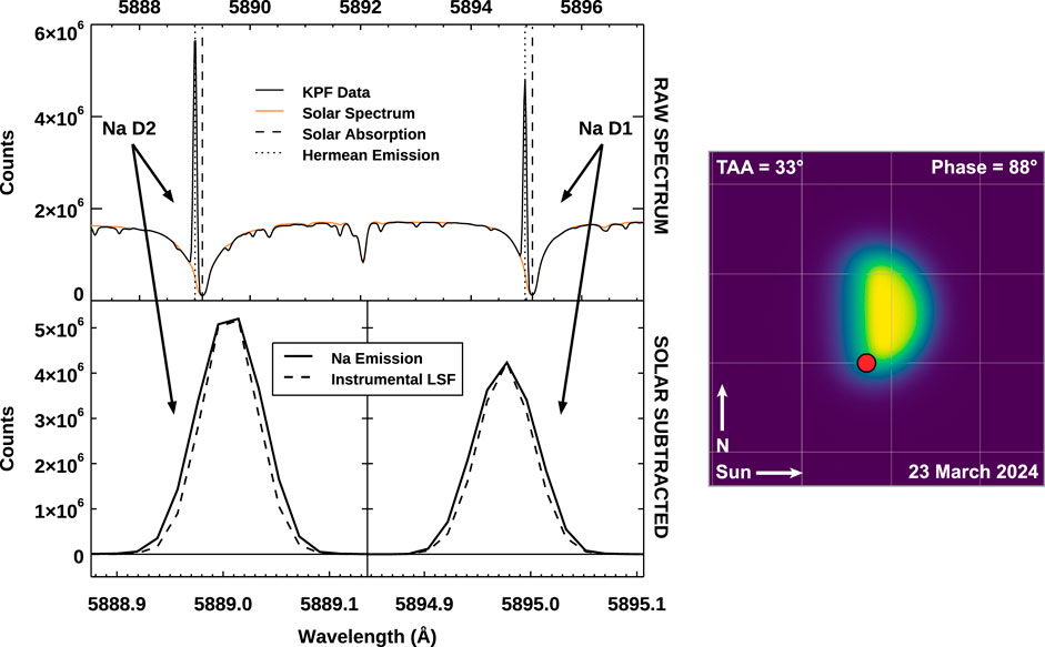
Figure 1. (Left) Spectrum of the sodium exosphere at Mercury’s south pole acquired with the KPF spectrometer on Keck 1. (Right) Guider image displaying Mercury’s dayside radiance with KPF fiber position in red.

Opacity is also important to consider, as saturation of the emission line core will result in fits to the Doppler broadening that overestimate the gas temperature. The stronger line in the sodium doublet, D2, saturates first, and so the line ratio between D2 and D1 can serve as a crude indicator of opacity effects. The optically thin ratio should be equivalent to the ratio in photon scattering rates, ∼1.6 for Na D2/D1, with a small correction for the D2 scattering phase function unique to a given observing geometry (Chamberlain, 1961; Equation 11.44). Saturation begins to occur in columns >10¹¹ cm^-2 and the line ratio approaches unity by 2 × 10¹² cm^-2. The D2/D1 line ratio of 1.25 in Figure 1 deviates from the theoretical value of 1.55, indicating that the column is moderately optically thick. Killen (2006) described a curve of growth model for such cases with applications near Mercury’s surface. Electron impact excitation has a different optically thin ratio of 2.0 since it scales with the state degeneracy alone and does not depend on the solar Fraunhofer spectrum. Electron excitation can be generally neglected for sodium and potassium in solar system exospheres, except in the case of Io (Schmidt et al., 2023), which is well known to be optically thick: two reasons why we omit it from the present discussion.

Pressure broadening is absent in planetary exospheres, and the natural width of <1 mK and Zeeman splitting can both be safely neglected. Thus, an observed line profile is a straightforward convolution of the Doppler broadened emission with the intrinsic instrumental line spread function (LSF). This LSF is wavelength dependent and can vary with a spectrograph’s environmental conditions. It can be quantified by imaging any source that closely enough approximates a delta function. In practice, such sources include cold spectral lamps like a Th-Ar hollow cathode or ideally a laser frequency comb. Either of these sources produce narrow emission lines across the optical range that are a good approximation of the spectrally local LSF. Variability from ambient conditions is combatted by acquiring these calibrations close in time to the science data.

2.2 Temperature derivation

Temperature can be derived from a Doppler-broadened emission line profile by one of two methods, depending on whether the profile is produced by a single transition or several hyperfine components. In the case of a single-component emission line, the absorption coefficient is the convolution of the negligibly narrow Lorentzian natural absorption profile with a Gaussian Doppler profile. Temperature, T, can be recovered for an optically thin transition centered at ${\lambda }_0$ as:

$T={\frac{m{c}^2}{8k\mathrm{l}\mathrm{n}\left(2\right)}\left(\frac{∆{\lambda }_D}{{\lambda }_0}\right)}^2(1)$

where k is Boltzmann’s constant, m is atomic mass, c is the speed of light, and $∆{\lambda }_D$ is the Gaussian full width at half maximum (FWHM). If the LSF is approximately Gaussian, the widths of these two components conveniently add in quadrature and so the Doppler width is $∆{\lambda }_D=\sqrt{{∆\lambda }_{Obs}^2-{∆\lambda }_{LSF}^2}$, where $∆{\lambda }_{Obs}$ is the observed line profile.

This standard reverse methodology cannot be applied for emission lines like sodium D that contain hyperfine structure; these line profiles are the summation of multiple hyperfine components, each with a unique transition strength and all with Doppler widths according to Equation 1. The first excited state of sodium is split by spin-orbit coupling, resulting in two transitions to ground, D1 = 5,896 Å and D2 = 5,890 Å. Each of these transitions is further split into several hyperfine components by anomalous Zeeman splitting, and the ground state is split. The resultant profile is a blend of these components, and so forward modeling is a more appropriate approach to recover an effective temperature.

To forward model an emission line, Equation 1 is first combined with a Maxwell-Boltzmann velocity distribution to derive a photon absorption coefficient for each hyperfine component:

${\alpha }_{\lambda }=\left(\frac{\pi e^2}{m_{e}c}\right)f\frac{2{\left(\ln 2\right)}^{\frac{1}{2}}}{\sqrt{\pi }\Delta {\lambda }_D}\exp \left[-\ln 2{\left(\frac{2\left(\lambda -{\lambda }_0\right)}{\Delta {\lambda }_D}\right)}^2\right](2)$

where m_e and e are the mass and charge of the electron and f is the transition’s unitless oscillator strength. Equation 2 is equivalent to the canonical work by Brown and Yung (1976) except for a factor of 2² inside of the exponential, which is present in their derivation but omitted in their Equation 15. Next, the total absorption profile can be generated by summing over all photon absorption coefficients. To retrieve temperature, this forward model can be convolved with the LSF and fit to an observed line profile, varying temperature to determine a best-fit. It is worth noting that the spread of published oscillator strengths of the sodium and potassium D hyperfine components introduces some uncertainty to this method. This study applies those weighted oscillator strengths reported by Brown and Yung (1976) for sodium and Welty et al. (1994) for potassium, which, when adjusted for the relative population of the ground states, are within 5% agreement with alternate reported values from Morton (2003), Steck et al., 2000, and Tiecke (2019).

For single component transition lines, reverse and forward methods match exactly. For sodium, however, approximation of the profile as a single component will overestimate temperature, as seen in Figure 2. At low temperatures, the disagreement is severe, while above 8000 K Doppler broadening dominates over the spacing of the hyperfine components. Hyperfine structure and ground state splitting in potassium D1 and D2 is less severe and so the two methods agree reasonably well above 2000 K, shown in Figure 3.

Figure 2

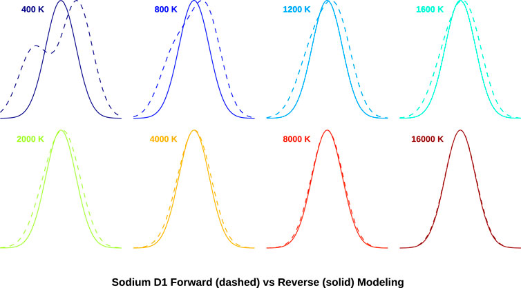
Figure 2. Forward and reverse modeled emission line profiles of the sodium D1 transition line at varying temperature. Forward modeling accounts for hyperfine structure that reverse modeling neglects, giving rise to the discrepancy between the two methods. The x-axes on these plots are scaled to the reverse model sigma, but in reality, these profiles are broadening significantly with temperature.

Figure 3

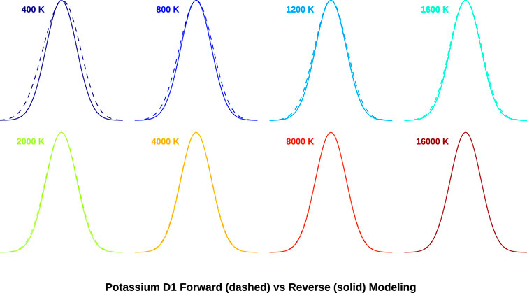
Figure 3. Forward and reverse modeled emission line profiles of the potassium D1 transition line at varying temperature. As with sodium, hyperfine structure causes a deviation from the theoretical profile of a single component line, but to a lesser degree.

While both of these methods assume a Maxwellian gas distribution, comparison of measured line profiles against theoretical profiles can test the validity of this assumption and reveal any non-thermal processes. Thermal equilibrium cannot be assumed for surface-bound exospheres, but the lack of collisions at these bodies has the useful quality that the energy distribution of exospheric particles resembles that of their source mechanism. Hence, a resolved line profile that agrees well with a thermal forward model would be suggestive of a thermal source producing the gas. Conversely, a measured profile fit poorly by a thermal model would suggest a non-thermal supply or loss mechanism acting on the gas population.

3 Linewidth comparisons in surface-bound exospheres

Three case studies where resolved sodium D line profiles vary as a function of altitude offer insightful comparison. The surface-bound exospheres of Mercury, the Moon, and Europa all exhibit dramatic Doppler broadening, but differences in morphology suggest three distinct causes. The observational details for each campaign are contained in Table 1. Again, temperature is not strictly defined for collisionless exospheres, so quoted values should be considered “effective temperatures” that assume a thermal population to provide a practical energy metric for the inherently nonthermal gas.

Table 1

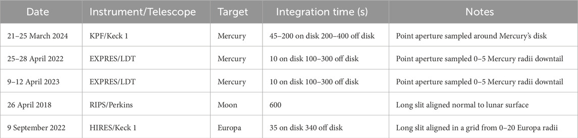
Table 1. Observational parameters.

3.1 Mercury

Intense sunlight at Mercury can both liberate atoms from the planet’s surface and then force them into an escaping comet-like tail (Ip, 1986; Smyth, 1986). The sodium exosphere was observed with KPF at the 10 m Keck one telescope from 22 to 23 March 2024 at True Anomaly Angle (TAA) 27°–34°. Observations were planned around greatest solar elongation, when Mercury’s tail is orthogonal to the line of sight, avoiding any projection effects and Doppler shifts associated with antisunward radiation acceleration. KPF resolved sodium line profiles across Mercury’s disk, but its resolving power is insufficient to constrain Doppler broadening in the narrower potassium D-lines, which are <1000 K here (Lierle et al., 2022). The 1.1″(730 km) diameter KPF fiber targeted seven regions around the disk and two down the exotail, while also probing one Mercury radius (R_M = 2,440 km) offset above the north and south poles to search for the hot scale height sodium population that Vervack et al. (2010) reported in MESSENGER limb scans.

The distribution of sodium temperatures is given in Figure 4. Quoted temperatures are the average of the individually forward modeled D1 and D2 lines, and the standard deviation of these individual temperatures gives the uncertainty. D2 temperatures are hotter than D1 everywhere on the dayside, as expected from its higher opacity, and deviation from optically thin line ratio. Using the opacity treatment in Schmidt et al. (2023) at 1200 K, the D2 line core reaches unity optical depth at 1.6 × 10¹¹ cm^-2 and twice this density for D1 (cf. Schmidt et al. (2023) Figure 11). The mean dayside measured D2/D1 ratio of 1.32 suggests the D2 is weakly saturated, and the optical depth at the D1 line core is very near unity. Consequently, the effective temperatures here cannot be accurately recovered without a more complex treatment, and values in Figure 4 are slightly overestimated near the dayside limb where the observed column densities are highest.

Figure 4

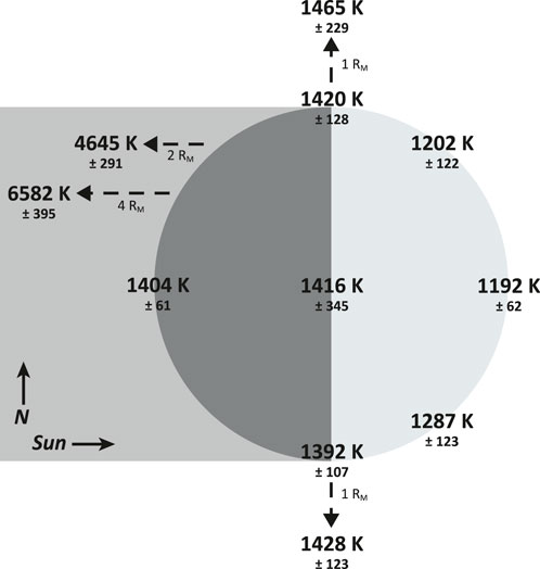
Figure 4. Linewidth based sodium effective temperatures at Mercury from PRV observations 23 March 2024. These values are the average of individual D1 and D2 temperatures, while quoted uncertainties are the standard deviation in these individual measurements and give a sense for column opacity.

With this caveat on opacity effects and the absolute sodium temperatures retrieved at Mercury, a relative trend in Figure 4 still emerges; sodium appears coldest near the sub-solar point, with temperatures increasing toward the nightside and poles. In this geometry, solar radiation pressure is 80 cm s^-2, or 22% of the surface gravity, and drives transport toward the nightside. We attribute the increase in effective temperature in the antisunward direction to the loss of low energy atoms to Mercury’s surface during transport. Most sodium atoms encountering the hot dayside surface are expected to bounce, but nearly 20% adsorb to smooth 500 K surfaces, and the regolith’s roughness increases this fraction (Yakshinskiy and Madey, 2005). Faster atoms in the source population will travel farther and encounter the surface fewer times during antisunward transport, allowing them to be retained while slower atoms are preferentially adsorbed. This produces an observational effect, where as the KPF line of sight is pointed farther from the subsolar point, more transport in the gas has occurred and more low velocity atoms are removed, broadening emission linewidths.

Despite opacity effects, the effective temperatures obtained from Doppler broadening in Figure 4 are in good agreement with values Cassidy et al. (2015) reported from atmospheric scale heights fit to MESSENGER Ultraviolet and Visible Spectrometer (UVVS) limb scans. They estimated 1200 K effective temperatures at the subsolar point and mid-afternoon equator, 1400 K above the south pole, and 1500 K at equatorial dawn. Figure 5 shows UVVS limb profiles tangent to points near equatorial dawn and in the same season as Figure 4. Sodium exhibits two distinct populations, one low-energy near the surface and one hotter above, with a sharp knee around 1,000 km tangent altitude. The altitude profile is fairly well approximated by the superposition (red line) of a low-lying component at the 1416 K KPF linewidth temperature and a more rarified population ∼2500 K. The temperature of this hot population is very poorly constrained and the analytic Chamberlain (1963) models applied in black do not account for ionization. While this hot component is clearly present beyond ∼1,000 km altitudes in UVVS measurements (Cassidy et al., 2015; Vervack et al., 2010), emission line profiles in the KPF dataset at 2,440 km tangent altitudes above Mercury’s poles surprisingly show no evidence of this population. This could be explained by the bright sodium emission below 1,000 km still dominating these observations at 2,440 km due to atmospheric seeing at high airmass expanding the 730 km fiber footprint. Very broad linewidths corresponding to effective temperatures of several thousand degrees, however, were observed at further distances antisunward, also shown in Figure 4.

Figure 5

Figure 5. Altitude profiles from the MESSENGER UVVS dataset (blue; Noam Izenberg, 2008) and Chamberlain line of sight models (black) that are superposed (red). UVVS data span orbit numbers 36 to 4,103 and YEARDOYs 2011095 to 2015120. The low energy population below 1,000 km tangent altitudes is fairly well reproduced by the 1416 K Doppler width at this location and season. The hot component at higher altitudes is not evident in resolved spectroscopy, and the 2500 K temperature prescribed here is poorly constrained.

Gas in Mercury’s escaping comet-like exotail was also observed during two campaigns with the R = 150,000 Extreme Precision Spectrometer (EXPRES; Jurgenson et al., 2016) on the 4.3 m Lowell Discovery Telescope in April 2022 and April 2023. In each campaign, the 0.9″(600 km) diameter EXPRES fiber was pointed once at disk center, followed by several integrations of up to 400 s stepping down the southern lobe of the exotail. Observations were again planned around greatest solar elongation, when Mercury’s exotail is orthogonal to the line of sight.

Sodium linewidths exhibit steep broadening from 0 (disk center) to 4.3 Mercury radii downtail, with derived effective temperatures given in Figure 6. On-disk line profiles are thermal in shape and again correspond to 1,200–1400 K, characteristic of sodium released from the surface by photon stimulated desorption (Yakshinskiy and Madey, 1999). Downtail, temperatures sharply increase before leveling off between 3 and 4 R_M. The two campaigns, occurring at true anomaly angle 56° and 80°, level off at near 7500 K and 5000 K, respectively. Discrepancy between D1 and D2 temperatures may be a systematic consequence of the hyperfine strengths and wavelengths applied, or any subtle variation in the instrumental LSF between the two D lines. Opacity effects are ruled out here due to rarified columns downtail.

Figure 6

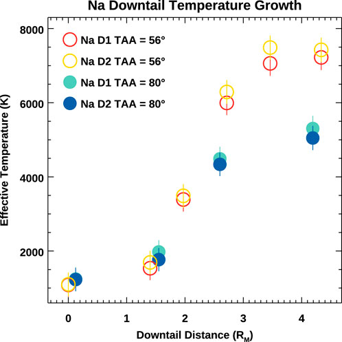
Figure 6. Sodium D1 and D2 effective temperatures increase dramatically down Mercury’s tail before leveling off around 3 - 4 R_M. Leveling off occurs at different effective temperatures for the two observed seasons, TAA = 56° and TAA = 80°.

This apparent heating in Mercury’s tail, even aside from its nonlinearity, is surprising. Such an effect is not predicted by the classic theory of planetary exospheres developed by Chamberlain (1963), and neutral and ion collisions are negligible in the tail. The only force not accounted for by Chamberlain (1963) is solar photon radiation pressure, which has a net direction orthogonal to the line of sight. The recoil momentum imparted during nearly isotropic photon re-emissions might be an explanation in principle, and atoms that Doppler shift into the solar continuum experience a constant scattering rate which could explain effective temperatures leveling off. Solar radiation acceleration, however, can only provide sufficient velocity to Doppler shift atoms from the Fraunhofer D wells into the solar continuum beyond 80 R_M downtail, far beyond the observed 3.5 R_M, effectively ruling out this explanation (Schmidt et al., 2010; Figure 6).

Instead, we interpret the observed broadening in Figure 6 not as heating, but again as an effect of Mercury’s gravity removing low energy atoms from the line of sight velocity distribution. When EXPRES is pointed at the disk, an approximately Maxwellian 1200 K source population is contained within the line of sight. As the line of sight moves farther and farther downtail, a smaller subset of only the hottest atoms from the source distribution are seen, since lower energy atoms are gravitationally bound below this altitude. Although added gravitational potential energy of these atoms, now at altitude, reduces their kinetic energy, this effect is primarily on the radial velocity component, while these observations are most sensitive to the tangential component. Additionally, although photon recoil momenta cannot explain these observations, strong radiation pressure still adds energy to the system, with atoms that are aloft for longer gaining more energy through sucessive scattering events. The interplay between gravity and radiation acceleration is difficult to quantify analytically, and so the importance of radiation acceleration to produce the observed line broadening is unknown. This interpretation is illustrated in Figure 7 and should occur, to some degree, everywhere around the planet, but the forcing of atoms into the exotail by radiation pressure enhances escape to a more measurable abundance and thus facilitiates observation. Figure 7 assumes a single thermal surface supply, an oversimplification of the true system, and as such is intended merely to convey the most general mechanics.

Figure 7

Figure 7. An illustration of gravity filtering the velocity distribution function with downtail distance. (Left) For three altitudes, the subset of the source distribution with energies high enough to reach the probed altitude is represented as the black curve, while the shaded region indicates the fraction of the original source population gravitationally bound below the line of sight. These distributions are not adjusted for the effects of gravity and radiation acceleration, and are only the fractions of the source distribution. Maxwell-Boltzmann flux distributions at the measured effective temperatures for each location are represented by dashed curves. v_orb and v_esc are the orbital and escape velocities, respectively. (Right) The increasingly nonthermal sodium D2 line profiles from EXPRES are shown in black for each altitude with forward models overlaid.

Gravitational filtering of the velocity distribution function is consistent also with the changing morphology of line profiles downtail, wherein line profiles transition from Gaussian to a rounded boxcar in shape, shown in Figure 7. Cold, low energy atoms comprise the core of an emission line, while hotter atoms make up the wings. It follows then, that as the coldest atoms are filtered out, the core of the emission line profile flattens while the wings remain, making it appear broader. Morphology of the emission line ceases to evolve when the population fully escapes. The leveling off point of the effective temperature near ∼3.5 R_M effectively marks the furthest extent of gravitationally bound sodium in the exosphere, beyond which all atoms escape, so no further filtering of the velocity distribution function is possible.

3.2 Moon

The lunar exosphere is qualitatively similar to that of Mercury with incident solar flux reduced by nearly an order of magnitude. A 2018 April campaign at the Perkins Telescope in Anderson Mesa, AZ targeted sodium in the Moon’s exosphere with the R = 137,000 Rapid Imaging Planetary Spectrograph (RIPS; Lierle et al., 2023). The spectrograph’s 42″long slit was oriented normal to the sunlit limb at the equator with 10-min integration times, such that changes with altitude could be measured directly along the slit. An on-disk spectrum was scaled and subtracted to isolate sodium emissions. RIPS lacks a ThAr hollow cathode calibration lamp, so a cold cathode neon discharge lamp was substituted to estimate the instrumental LSF for each pixel row. This corrects for any non-uniform focus along the slit, and resultant Doppler widths were then forward modeled at each pixel row to derive the local effective temperature. These are shown vs. tangent altitude in Figure 8 over a 70 km region above the sunlit equatorial limb where the lunar disk was 84% illuminated.

Figure 8

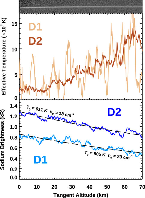
Figure 8. (Top) An isolated 2D lunar sodium D2 profile showing visible broadening along the long slit. (middle) Sodium D linewidths increasing steeply from ∼2000 K near the surface to nearly 10,000 K at 70 km above the lunar limb. (Bottom) Simultaneous measurements of the sodium brightness distribution are fit by Chamberlain (1963) models and exhibit e-folding scale heights of 150–200 km.

As observed at Mercury, sodium linewidth temperatures increase with distance from the Moon, but much more sharply. This is seen more robustly in D2 (median uncertainty of 992 K), since it is about 50% brighter than D1 (median uncertainty of 2157 K). Variations in sodium linewidths on local scales near the surface have not been reported previously, and Doppler broadening is known to be relatively constant at higher altitudes (Kuruppuaratchi et al., 2018). Linewidth morphology on these distance scales cannot be attributed purely to gravitational filtering; effective temperatures double over 4,300 km in the above measurements at Mercury, whereas nearly a factor of 5 increase is observed here over just 70 km. In the lunar case, alternative explanations to gravitational partitioning of the velocity distribution function are necessary.

Like at Mercury, a cold sodium population has been observed near the Moon’s surface (Potter and Morgan, 1988b; Sprague et al., 2012) which is attributed to photon stimulated desorption (Yakshinskiy and Madey, 1999), while a hot component thought to be sourced by either micrometeoroid vaporization or plasma sputtering (Kuruppuaratchi et al., 2018) dominates at higher altitudes. A potential explanation for the steeply increasing effective temperature in Figure 8 is that this observation sampled the transition region between the two, where neither source is dominant. The “knee” at the transition region near 1,000 km in Figure 5 would be difficult to distinguish on small spatial scales. This interpretation would require comparable ejection rates between hot and cold source mechanisms. If the cold photodesorbed abundance at Mercury depicted in Figure 5 were adjusted by factor of 10 corresponding to the reduced solar irradiance at the Moon, then comparable contributions from these same hot and cold sources might be expected. However, an appropriate scaling of the hot component between Mercury and the Moon is not obvious. Moreover, surface Na available for desorption is in the topmost monolayers, whereas energetic sources excavate from depth, and these distributions within the regolith likely differ between the two bodies.

Brightness versus altitude profiles in Figure 8 are fit with analytic models shown in black dashed lines to derive temperature and volume density at the surface (J. W. Chamberlain, 1963). These profiles exhibit e-folding scale heights of 150–200 km, which are comparable to the ∼90 km values that Cassidy et al. (2015) reported at Mercury considering the factor of 2.3 difference in surface gravity. The lunar D1 falloff is best fit by a 505 K population with n₀ = 23 cm^-3 and D2 with a 611 K source with n₀ = 18 cm^-3. This is in tension with the linewidth derived temperatures of >2000 K near the surface, which is surprising, since the only similar measurement by Potter and Morgan (1988a) found good agreement between temperatures measured with both these methods. Their D2 scale heights correspond to a sodium temperature of 540 K, which they state would result in effective line broadening of 40 mÅ FWHM, consistent to their resolved 42 mÅ D2 linewidths. The derived scale height temperatures herein match well, but the linewidth temperatures are discrepant.

Cold gas temperatures derived from linewidth measurements are especially sensitive to 1) the accuracy of the applied instrumental linewidth and 2) the hyperfine structure used to model the line profile. While both types of Th-Ar and Ne lamps effectively produce delta functions at ambient room-temperature, Ne produces fewer strong lines near the Na doublet. We use interpolation from fits to multiple Ne lines to determine the local LSF at each of the D lines. Since the methodology for determining LSF is not standardized between different studies, even subtle differences in LSF may produce significant differences in temperature. Independent is the issue of assumed hyperfine structure; Potter and Morgan (1988b) calculate that a 540 K line is theoretically broadened to 40 mÅ, while the forward model applied herein at this temperature has a 35 mÅ width. Though this 5 mÅ difference may seem insignificant, a 1200 K temperature is then necessary to produce 40 mÅ D2 widths. This discrepancy may reflect different assumed oscillator strengths and line centers for the sodium hyperfine structure. Present work applies those determined by Brown and Yung (1976), which, when accounting for the applied statistical weights “gf” of the hyperfine ground state, match those more recently published by Morton (2003) within 5%. Differing treatments of these two aspects may impart systematic errors in the absolute Doppler width reported between independent studies, but would not affect the relative morphology in Figure 8.

Observing geometry in an exosphere that is not spherically symmetric is another consideration for interpreting the apparent discrepancy between temperature derivation methods in Figure 8. With the Moon near full in its waxing gibbous phase, the RIPS line of sight passed through some of the escaping lunar sodium tail. Atoms in the escaping tail can glow more brightly due to their higher photon scattering frequencies. In this observing geometry, radiation acceleration imparts an antisunward velocity that is not orthogonal to the line of sight, unlike the Mercury cases above. This forcing would manifest differently between the Doppler broadening and the altitude distribution. Modeling and further observations as a function of lunar phase are needed to evaluate how projection effects through the lunar exotail affect scale height and Doppler width near the lunar limb.

A final consideration is thermal accommodation during gas-surface interactions. In this scenario, bouncing atoms might lose energy via inelastic surface collisions with the colder surface, and a single hot source population would produce narrow linewidths near the surface and broader lines at altitude. Accommodation with the local surface temperature may require many bounces and not reach equilibrium before adsorption. Evidence at Mercury does not support this explanation, as the “knee” in Figure 5 indicates two distinct sources without the continuum of energies expected from inelastic collisions. MESSENGER analysis found no evidence for a thermalized component near Mercury’s surface (Cassidy et al., 2015), and exosphere models suggest that any accommodation towards the local surface temperature during bouncing is weak (Burger et al., 2010; Mouawad et al., 2011; Schmidt, 2013).

3.3 Europa

There have been comparatively few observations of Europa’s sodium exosphere: none space-based, and Leblanc et al. (2005) summarize all past ground-based measurements. An observing campaign on 29 September 2022 measured Europa’s extended alkali exosphere near the satellite’s eastern elongation from Jupiter with the High Resolution Echelle Spectrograph (HIRES; Vogt et al., 1994) at the Keck one telescope. The instrumental mode used a 28″long slit at R∼50,000 resolving power. After subtraction of scattered sunlight, the radial profile of sodium effective temperatures in Figure 9 was generated from multiple spectra pointing both on and off Europa’s disk in a grid-like pattern. Due to the small angular size of Europa’s disk (1.09″diameter) and its high optical albedo, faint emissions cannot be recovered within a few Europa radii (R_E) of the surface; however, the exosphere falls off slowly. Emissions were measured beyond 30 R_E and can be distinguished from Io and telluric contamination by Doppler shift.

Figure 9

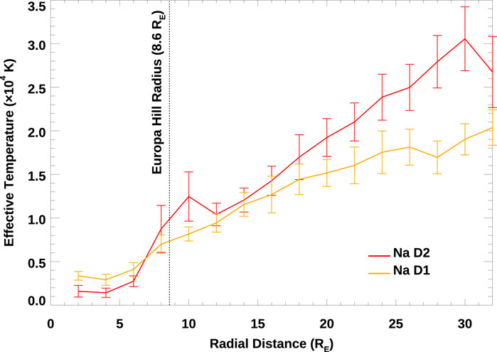
Figure 9. Sodium D1 (orange) and D2 (red) linewidths increasing with radial distance from Europa. Line profiles continue to broaden past Europa’s 8.6 R_E Hill radius (dotted line), all the way out to 30 R_E.

Sodium effective temperatures derived from Doppler widths in Europa’s extended exosphere are hotter than seen at the Moon or Mercury, and again they increase with distance from Europa’s surface. Effective temperatures close to the surface are near the limiting instrumental resolution in range of a few thousand Kelvin. The Doppler width of the lines far from Europa cannot be attributed to the gravitational filtering effects illustrated above for Mercury. Europa’s Hill sphere lies at ∼8.6 R_E where Jupiter’s gravity dominates over that of Europa itself, but emission linewidths broaden well beyond this boundary. The atmospheric scale height at Europa has not been previously measured and the measurements here do not offer useful constraints on the energy since the 1/R slope is consistent with a population that is essentially fully escaping.

At Europa’s 2 km s^-1 escape velocity, the time to travel the observed distance scales is a few hours. Cumulative effects of radiation acceleration will broaden the sodium D lines on these time scales. Since atoms along the line of sight have a distribution of different ages and heliocentric velocities, the effects of radiation acceleration do not impart velocity uniformly. Sodium atoms are accelerated by 1–2 cm s^-2, with more than a day’s time necessary to achieve the Doppler broadening of 1 km s^-1, by which time the atoms are beyond the observed region. Thus, while this effect is non-negligible, radiation acceleration fails to explain the observation. Ion-neutral momentum transfer in the Jovian magnetosphere, known to impart winds of a few hundred m s^-1 on Io’s atmosphere (Thelen et al., 2024), offers another possible explanation. At Io, it is an effect of charge exchange type interactions (Banks, 1966), in which neutral products can collisionally distribute their momentum. This would seem inefficient in Europa’s exosphere, and require detailed modeling to quantify (Smith et al., 2019). Since Jovian gravity dominates, the Keplerian dynamics of escaping atoms must also be considered. Atoms escaping Europa’s trailing hemisphere fall inward towards Jupiter whereas leading hemisphere escape overtakes Europa’s orbital motion and drifts radially outward. Straightforward explanations of the measured Doppler broadening in Figure 9 are not altogether forthcoming when considering Keplerian orbits. Monte Carlo simulations are perhaps a more viable approach, and treatment must account for the ∼20-h electron impact ionization lifetime (Burger and Johnson, 2004; Leblanc et al., 2005). A detailed analysis of these mechanics is beyond the scope of this paper, but there is much to be learned from a further study into this host planet’s influence on its satellite’s exosphere.

4 Conclusion

Sodium D line profiles exhibit measurable Doppler broadening with increasing altitude in the surface-bound exospheres of Mercury, the Moon, and Europa. Each is prescribed to different effects and occurs at different scales. At Mercury, apparent broadening is due to gravity removing the lowest energy atoms from the observed line-of-sight velocity distribution function. Growth in Doppler broadening ceases at the ballistic apex of bound atomic trajectories, effectively defining a boundary beyond which all gas escapes. At the Moon, sharply increasing sodium linewidths are observed over an altitude range far too small for significant differences in the partitioning of bound and escaping gas, necessitating an alternative explanation. Possibilities include projection effects through the line of sight, measurements that sampled a transition region between multiple source populations, and/or the thermal accommodation of a single hot source towards the colder surface temperatures. At Europa, broadening sodium line profiles well beyond the satellite’s Hill radius suggest that Jovian gravity or magnetospheric plasma can influence the altitudinal velocity distribution of its escaping exosphere.

These three cases form the basis for a further investigation in comparative aeronomy to understand how the processes involved in exosphere morphology shape the exosphere under different conditions: close to the Sun, partially shielded by Earth’s magnetosphere, or fully embedded in the Jovian gravity and magnetospheric plasma.

Data availability statement

The KPF and HIRES data analyzed within this work are available on the W. M. Keck Observatory Archive (a29hLmlwYWMuY2FsdGVjaC5lZHU=). Mercury spectra from EXPRES are publicly archived at doi.org/10.5281/zenodo.14728009.

Author contributions

PL: Conceptualization, Data curation, Formal analysis, Funding acquisition, Investigation, Methodology, Project administration, Resources, Software, Validation, Visualization, Writing – original draft, Writing – review and editing. EL: Conceptualization, Data curation, Formal analysis, Funding acquisition, Investigation, Methodology, Resources, Software, Validation, Visualization, Writing – original draft, Writing – review and editing. CS: Conceptualization, Data curation, Formal analysis, Funding acquisition, Investigation, Methodology, Project administration, Resources, Software, Supervision, Validation, Visualization, Writing – original draft, Writing – review and editing. AM: Data curation, Funding acquisition, Writing – review and editing.

Funding

The author(s) declare that financial support was received for the research and/or publication of this article. This material is based upon work supported by the National Aeronautics and Space Administration. PL acknowledges support from JPL RSA# 1707133 for Keck KPF measurements. EL acknowledges support from the FINESST Fellowship under award 80NSSC23K1642. CS and AM acknowledge support under award 80NSSC21K1019. CS acknowledges support under awards 80NSSC22K1303 and 80NSSC21K0051.

Acknowledgments

We thank the KPF instrument team, particularly Howard Isaacson and Jack Wright, as well as staff astronomer Josh Walawender, for welcoming the challenge of observing Mercury. We also thank members of the EXPRES instrument team, particularly Debra Fischer, John Michael Brewer, Lily Zhao, Ryan Blackman, Allen Davis, Ryan Petersburg, and Andrew Szymkowiak, for their support of the observations at LDT and assistance with the data analysis. We gratefully acknowledge the help of Dr. Aimee Merkel for providing MESSENGER UVVS sodium emission data at Mercury and Dr. Tim Cassidy for sharing IDL code to calculate the line of sight density predicted by Chamberlain’s (1963) theory. Some of the data presented herein were obtained at Keck Observatory, which is a private 501(c)3 non-profit organization operated as a scientific partnership among the California Institute of Technology, the University of California, and the National Aeronautics and Space Administration. The Observatory was made possible by the generous financial support of the W. M. Keck Foundation. The authors wish to recognize and acknowledge the very significant cultural role and reverence that the summit of Maunakea has always had within the Native Hawaiian community. We are most fortunate to have the opportunity to conduct observations from this mountain.

Conflict of interest

The authors declare that the research was conducted in the absence of any commercial or financial relationships that could be construed as a potential conflict of interest.

The handling editor DB declared a past co-authorship with the author CS.

Generative AI statement

The author(s) declare that no Generative AI was used in the creation of this manuscript.

Publisher’s note

All claims expressed in this article are solely those of the authors and do not necessarily represent those of their affiliated organizations, or those of the publisher, the editors and the reviewers. Any product that may be evaluated in this article, or claim that may be made by its manufacturer, is not guaranteed or endorsed by the publisher.

References

Banks, P. (1966). Collision frequencies and energy transfer. Ions. Planet. Space Sci. 14 (11), 1105–1122. doi:10.1016/0032-0633(66)90025-0

CrossRef Full Text | Google Scholar

Bridge, H. S., Belcher, J. W., Lazarus, A. J., Olbert, S., Sullivan, J. D., Bagenal, F., et al. (1981). Plasma observations near Saturn: initial results from voyager 1. Sci 212 (4491), 217–224. doi:10.1126/SCIENCE.212.4491.217

PubMed Abstract | CrossRef Full Text | Google Scholar

Brown, R. A., and Yung, Y. L. (1976). Io, its atmosphere and OPTICAL EMISSIONS. Tucson: University of Arizona Press.

Google Scholar

Burger, M. H., and Johnson, R. E. (2004). Europa’s neutral cloud: morphology and comparisons to Io. Icarus 171 (2), 557–560. doi:10.1016/J.ICARUS.2004.06.014

CrossRef Full Text | Google Scholar

Burger, M. H., Killen, R. M., Vervack, R. J., Bradley, E. T., McClintock, W. E., Sarantos, M., et al. (2010). Monte carlo modeling of sodium in Mercury’s exosphere during the first two MESSENGER flybys. Icarus 209 (1), 63–74. doi:10.1016/j.icarus.2010.05.007

CrossRef Full Text | Google Scholar

Cassidy, T. A., Merkel, A. W., Burger, M. H., Sarantos, M., Killen, R. M., McClintock, W. E., et al. (2015). Mercury’s seasonal sodium exosphere: MESSENGER orbital observations. Icarus 248, 547–559. doi:10.1016/j.icarus.2014.10.037

CrossRef Full Text | Google Scholar

Chamberlain, J. W. (1961). Physics of the Aurora and airglow (International Geoph). Academic Press.

Google Scholar

Chamberlain, J. W. (1963). Planetary coronae and atmospheric evaporation. Pktw. Space Sci. 11, 901–960. doi:10.1016/0032-0633(63)90122-3

CrossRef Full Text | Google Scholar

Chamberlain, J. ∼W., and Hunten, D. ∼M. (1987). Theory of planetary atmospheres: an introduction to their physics and chemistry/2nd revised and enlarged edition, 36. Orlando FL Academic Press Inc International Geophysics Series.

Google Scholar

Coddington, O. M., Richard, E. C., Harber, D., Pilewskie, P., Woods, T. N., Chance, K., et al. (2021). The TSIS-1 hybrid solar reference spectrum. GeoRL 48 (12), e2020GL091709. doi:10.1029/2020GL091709

PubMed Abstract | CrossRef Full Text | Google Scholar

Gibson, S. R., Howard, A. W., Marcy, G. W., Edelstein, J., Wishnow, E. H., and Poppett, C. L. (2016). “KPF: Keck planet finder,” in KPF: Keck planet finder, 9908. SPIE. doi:10.1117/12.2233334990870

CrossRef Full Text | Google Scholar

Hunten, D. M., and Hunten, and M. D. (1973). The escape of light gases from planetary atmospheres. JAtS 30 (8), 1481–1494. doi:10.1175/1520-0469(1973)030<1481:TEOLGF>2.0

CrossRef Full Text | Google Scholar

Ip, W.-H. (1986). The sodium exosphere and magnetosphere of mercury. Geophys. Res. Lett. 13 (5), 423–426. doi:10.1029/GL013I005P00423

CrossRef Full Text | Google Scholar

Jurgenson, C., Fischer, D., McCracken, T., Sawyer, D., Szymkowiak, A., Davis, A., et al. (2016). EXPRES: a next generation RV spectrograph in the search for earth-like worlds. SPIE 9908, 99086T. doi:10.1117/12.2233002

CrossRef Full Text | Google Scholar

Killen, R. M. (2006). Curve-of-Growth model for sodium D2 emission at mercury. Publ. Astronomical Soc. Pac. 118 (847), 1344–1350. doi:10.1086/508070

CrossRef Full Text | Google Scholar

Killen, R. M., Potter, A., Fitzsimmons, A., and Morgan, T. H. (1999). Sodium D2 line profiles: clues to the temperature structure of Mercury’s exosphere. Planet. Space Sci. 47 (12), 1449–1458. doi:10.1016/S0032-0633(99)00071-9

CrossRef Full Text | Google Scholar

Kuruppuaratchi, D. C. P., Mierkiewicz, E. J., Oliversen, R. J., Sarantos, M., Derr, N. J., Gallant, M. A., et al. (2018). High-resolution, ground-based observations of the lunar sodium exosphere during the lunar atmosphere and dust environment explorer (LADEE) mission. J. Geophys. Res. Planets 123 (9), 2430–2444. doi:10.1029/2018JE005717

CrossRef Full Text | Google Scholar

Leblanc, F., Potter, A. E., Killen, R. M., and Johnson, R. E. (2005). Origins of europa Na cloud and torus. Icarus 178 (2), 367–385. doi:10.1016/J.ICARUS.2005.03.027

CrossRef Full Text | Google Scholar

Lierle, P., Schmidt, C., Baumgardner, J., Moore, L., Bida, T., and Swindle, R. (2022). The spatial distribution and temperature of mercury’s potassium exosphere. Planet. Sci. J. 3 (4), 87. doi:10.3847/PSJ/AC5C4D

CrossRef Full Text | Google Scholar

Lierle, P., Schmidt, C., Baumgardner, J., Moore, L., and Lovett, E. (2023). Rapid imaging planetary spectrograph. Publ. Astronomical Soc. Pac. 135 (1051), 095002. doi:10.1088/1538-3873/acec9f

CrossRef Full Text | Google Scholar

Morton, D. C. (2003). Atomic data for resonance absorption lines. III. Wavelengths longward of the lyman limit for the elements hydrogen to gallium. ApJS 149 (1), 205–238. doi:10.1086/377639

CrossRef Full Text | Google Scholar

Mouawad, N., Burger, M. H., Killen, R. M., Potter, A. E., McClintock, W. E., Vervack, R. J., et al. (2011). Constraints on Mercury’s Na exosphere: combined MESSENGER and ground-based data. Icarus 211 (1), 21–36. doi:10.1016/j.icarus.2010.10.019

CrossRef Full Text | Google Scholar

Niemann, H. B., Hartle, R. E., Kasprzak, W. T., Spencer, N. W., Hunten, D. M., and Carignan, G. R. (1979). Venus upper atmosphere neutral composition: preliminary results from the pioneer Venus orbiter. Science 203 (4382), 770–772. doi:10.1126/SCIENCE.203.4382.770

PubMed Abstract | CrossRef Full Text | Google Scholar

Noam Izenberg (2008). Messenger E/V/H mascs 3 UVVS calibrated data V1.0. NASA Planetary Data System. (MESS-E/V/H-MASCS-3-UVVS-CDR-CALDATA-V1.0).

Google Scholar

Potter, A. E., and Morgan, T. H. (1988a). Discovery of sodium and potassium vapor in the atmosphere of the moon. New Ser. 241, 675–680. doi:10.1126/science.241.4866.675

PubMed Abstract | CrossRef Full Text | Google Scholar

Potter, A. E., and Morgan, T. H. (1998b). Coronagraphic observations of the lunar sodium exosphere near the lunar surface. J. Geophys. Res. Planets 103 (E4), 8581–8586. doi:10.1029/98JE00059

CrossRef Full Text | Google Scholar

Rosborough, S. A., Oliversen, R. J., Mierkiewicz, E. J., Sarantos, M., Robertson, S. D., Kuruppuaratchi, D. C. P., et al. (2019). High-resolution potassium observations of the lunar exosphere. Geophys. Res. Lett. 46 (12), 6964–6971. doi:10.1029/2019GL083022

CrossRef Full Text | Google Scholar

Schmidt, C. A. (2013). Monte carlo modeling of north-south asymmetries in Mercury’s sodium exosphere. J. Geophys. Res. Space Phys. 118 (7), 4564–4571. doi:10.1002/jgra.50396

CrossRef Full Text | Google Scholar

Schmidt, C. A., Wilson, J. K., Baumgardner, J., and Mendillo, M. (2010). Orbital effects on Mercury’s escaping sodium exosphere. Icar 207 (1), 9–16. doi:10.1016/J.ICARUS.2009.10.017

CrossRef Full Text | Google Scholar

Schmidt, C., Sharov, M., de Kleer, K., Schneider, N., de Pater, I., Phipps, P. H., et al. (2023). Io’s optical aurorae in jupiter’s shadow. Planet. Sci. J. 4 (2), 36. doi:10.3847/PSJ/AC85B0

CrossRef Full Text | Google Scholar

Slanger, T. G., and Osterbrock, D. E. (2000). Investigations of potassium, lithium, and sodium emission in the nightglow and OH cross calibration. J. Geophys. Res. Atmos. 105 (D1), 1425–1429. doi:10.1029/1999JD901027

CrossRef Full Text | Google Scholar

Smith, H. T., Mitchell, D. G., Johnson, R. E., Mauk, B. H., and Smith, J. E. (2019). Europa neutral torus confirmation and characterization based on observations and modeling. Astrophysical J. 871 (1), 69. doi:10.3847/1538-4357/aaed38

CrossRef Full Text | Google Scholar

Smyth, W. H. (1986). Nature and variability of Mercury’s sodium atmosphere. Nature 323 (6090), 696–699. doi:10.1038/323696A0

CrossRef Full Text | Google Scholar

Sprague, A. L., Sarantos, M., Hunten, D. M., Hill, R. E., and Kozlowski, R. W. H. (2012). The lunar sodium atmosphere: april–may 1998 ¹This article is part of a special issue that honours the work of dr. Donald M. Hunten FRSC who passed away in December 2010 after a very illustrious career. CaJPh 90 (8), 725–732. doi:10.1139/P2012-072

CrossRef Full Text | Google Scholar

Steck, D. A. (2000). Sodium D line data.

Google Scholar

Thelen, A. E., Kleer, K. de, Cordiner, M. A., Pater, I. de, Moullet, A., and Luszcz-Cook, S. (2024). Io’s SO2 and NaCl wind fields from ALMA. Astrophysical J. Lett. 978 (1), L1. doi:10.3847/2041-8213/AD9BB5

CrossRef Full Text | Google Scholar

Tiecke, T. G. (2019). Properties of potassium. Available online at: https://www.tobiastiecke.nl/archive/PotassiumProperties.pdf.

Google Scholar

Vervack, R. J., McClintock, W. E., Killen, R. M., Sprague, A. L., Anderson, B. J., Burger, M. H., et al. (2010). Mercury’s complex exosphere: results from mESSENGER’s third flyby. Sci 329 (5992), 672–675. doi:10.1126/SCIENCE.1188572

PubMed Abstract | CrossRef Full Text | Google Scholar

Vogt, S. S., Allen, S. L., Bigelow, B. C., Bresee, L., Brown, W. E., Cantrall, T., et al. (1994). “HIRES: the high-resolution echelle spectrometer on the keck 10-m telescope,” in Instrumentation in astronomy VIII, 2198. doi:10.1117/12.176725

CrossRef Full Text | Google Scholar

Welty, D. E., Hobbs, L. M., and Kulkarni, V. P. (1994). A high-resolution survey of interstellar NA I D1 lines. Astrophysical J. 436, 152. doi:10.1086/174889

CrossRef Full Text | Google Scholar

Yakshinskiy, B. V., and Madey, T. E. (1999). Photon-stimulated desorption as a substantial source of sodium in the lunar atmosphere. Nat. 1999 400 (6745), 642–644. doi:10.1038/23204

PubMed Abstract | CrossRef Full Text | Google Scholar

Yakshinskiy, B. V., and Madey, T. E. (2005). Temperature-dependent DIET of alkalis from SiO2 films: Comparison with a lunar sample. Surf. Sci. 593 (1–3), 202–209. doi:10.1016/j.susc.2005.06.062

CrossRef Full Text | Google Scholar