The hydrogen Lyman α line shape in the exospheres of terrestrial objects in the solar system

The exospheres of all objects are mostly made of atomic hydrogen. Because the Sun is bright in Lyman α, the properties of the H atoms in the exospheres of certain terrestrial solar system objects can be studied by analyzing the resonantly scattered solar Lyman α emission by these exospheric H atoms. This emission is optically thick in the exospheres of all planets in our solar system except Mercury. This makes it complicated to derive the true characteristics (number density distribution, energy distribution) of the H atoms present in these exospheres. While radiative transfer (RT) models have been used extensively to derive the characteristics of exospheric H atoms by modeling the line-integrated Lyman α intensity measured by spacecrafts via remote sensing, the models often fail to resolve discrepancies between the observed emission intensity and the simulated value. This is because of the various assumptions that are made in the RT models about the inherent characteristics of the H atoms and the corresponding Lyman α lineshape. Our knowledge about the characteristics of the H atoms can be significantly improved by understanding what the true lineshape of the H Lyman α line may be for various conditions. This can then be used to resolve the discrepancies between the modeled and the observed intensities for planetary exospheres. Here we present a detailed study on the shape of the exospheric Lyman α emission line for various conditions like change in altitude, temperature, non-isothermality, asymmetry, and presence of non-thermal atoms. These detailed line profiles are being used to determine H density distribution in Earth’s exosphere from analysis of absorption of the solar Lyman α line by geocoronal H as measured by remote sensing satellites. This theoretical analysis also highlights the advantages of obtaining highly resolved H Lyman α emission line measurements from the exospheres of certain terrestrial objects in our solar system.

1 Introduction

Atomic hydrogen (H) is ubiquitous in the exospheres of every planet and satellite in our solar system. Studying this layer can provide important insights into an object’s atmospheric dynamics, escape, photochemistry, composition and evolution history with time. For example, at Mars the H escape rate is an important marker of the water escape history of the planet (Jakosky et al., 2018). At Earth the interaction of atomic H with the plasmasphere specifically during geomagnetic storm events is a crucial tracer of the space weather effects on Earth’s upper atmospheric dynamics (Ilie et al., 2013; Krall et al., 2018). At Venus, exospheric hydrogen is produced by chemical reactions involving hydrogen-bearing molecules which play an important role in the photochemistry of the mesosphere-thermosphere region (Krasnopolsky, 2008; Yung and Demore, 1982). At the Galilean moons, observations of the H corona provide information on the surface ice content of these objects (Roth et al., 2017; Carberry Mogan et al., 2022). The scientific value of studying exospheric hydrogen atoms has been recognized by the research community allowing for dedicated NASA missions like the Carruthers Geocorona Observatory (CGO), or instruments like the Imaging Ultraviolet Spectrograph (IUVS) on the Mars Atmosphere and Volatile Evolution mission (MAVEN) with low and high resolution channels for investigating atomic H as well as allocating Hubble Space Telescope (HST) time towards studying exospheric H in the solar system (Clarke et al., 2014; Clarke et al., 2017; Clarke et al., 2024; Chaffin et al., 2015; Bhattacharyya et al., 2015; Bhattacharyya et al., 2020; Bhattacharyya et al., 2023; Roth et al., 2017).

One of the easiest and most-pursued methods of characterizing exospheric H atoms is by observing the Lyman α emission from the exospheres of different objects. The energy of the Lyman α photon represents the transition energy between the ground and the first excited state in the hydrogen atom. Because the sun is very bright at Lyman α, the solar Lyman α photon readily undergoes resonant scattering by the H atoms present in the exospheres of solar system bodies (Milligan, 2021). Lyman α observations are generally conducted via remote sensing either with low resolution spectrographs (Bertaux et al., 2006; 2007; McClintock et al., 2015; Paxton et al., 2004; Broadfoot et al., 1977) or with broadband imagers sensitive to the far-ultraviolet (FUV) wavelength range (Clarke et al., 2009; Clarke et al., 2014; Bhattacharyya et al., 2015; Kameda et al., 2017). These low-resolution spectral observations or broadband images provide line of sight (LOS) intensities which are integrated over the entire shape of the exospheric H Lyman α line. For bodies with thin atmospheres (optical depth τ < 1), it is easy to derive the H column densities because the coronal H Lyman α emission is optically thin, i.e., H column density along a LOS is directly proportional to the observed LOS H Lyman α intensity. But for bodies with thicker atmospheres (τ > 1), the observed brightness needs to be modeled with radiative transfer theory accounting for multiple scattering effects undergone by the solar Lyman α photons in the hydrogen exosphere of such bodies. A lot of key characteristics about the exospheric H atoms may be lost in translation due to the various assumptions made in the modeling process and the uncertainties brought on by the degeneracy between the unknown parameters of temperature and number density on the observed column integrated intensity (Bhattacharyya et al., 2017; Chaffin et al., 2018). These factors make it difficult to characterize the density and the energy distribution of H atoms in optically thick exospheres.

Resolving the exospheric H Lyman α line, on the other hand, may provide unprecedented information about the true nature of the H atoms present in the exospheres of objects with thick atmospheres. To date there exists no measurements of the exospheric H Lyman α emission at a resolution higher than R∼25,000. There does exist measurements of the H Balmer α line at Earth with the Wisconsin H alpha Mapper (WHAM) at an R ∼37,000–80,000 (Mierkiewicz et al., 2006). However, the H Balmer α line is much lower in intensity than the H Lyman α line (>1,000 times lower) and is restricted by observing geometry with most observations being conducted on the nightside with solar depression angles >20° (Gardner et al., 2017). Even then the H Balmer α observations have revealed important details about the behavior of the geocorona with solar cycle variations and changing exospheric temperature with altitude at R ∼37,000–80,000 (Nossal et al., 2004; Nossal et al., 2008; Mierkiewicz et al., 2012). Because our knowledge about the characteristics of exospheric H atoms can be significantly improved by determining the true lineshape of the exospheric H Lyman α line at high resolution, here we present a detailed theoretical study of the information that can be obtained for objects with optically thick exospheres (1 < τ < 500) at Lyman α with knowledge of the H Lyman α lineshape at a very high resolution (R > 175,000). The results from the theoretical model are currently being used to derive exospheric column H densities by analyzing the solar H Lyman α absorption signal instead of the typical coronal H Lyman α emission signal at Earth with data from the Extreme Ultraviolet and Irradiance Sensors (EXIS) onboard the National Oceanic and Atmospheric Administration (NOAA) Geostationary Operational Environmental Satellite (GOES) (Machol et al., 2021; Thiemann et al., 2021).

This paper presents a description of the model used to calculate the H Lyman α lineshape at high resolution and includes a detailed analysis of the effect of various conditions like spacecraft observing geometry, inherent temperature and density distribution assumptions for an exosphere and the presence of non-thermal H atoms on the H Lyman α lineshape. The study presented here will help in the interpretation of actual observations of the H Lyman α lineshape that may be obtained by future instruments such as a Spatial Heterodyne Spectrometer (Harris et al., 2024) or a Fourier Transform Spectrograph (De Oliveira et al., 2009; De Oliveira et al., 2011) which can operate at a much higher resolution in the FUV wavelength range (R > 175,000) than the presently available spectrographs.

2 Model description

The spectral lineshape of the H Ly-a line along any line of sight for an exosphere can be studied by determining the velocity distribution of the atoms along the line-of-sight column. The study presented here considers optical depths of 1 < τ < 500 at line center (Meier, 1991). This encompasses the exospheres of Venus, Earth, Mars, Titan, and Pluto. We do not consider the much thicker exospheres of the Gas Giants and the Ice Giants or the tenuous atmospheres of bodies like Mercury and the Galilean moons in this study. For the giant planets the large amount of hydrogen in their atmospheres saturates the line center and the contribution from the natural wings of the line then comes into play which complicates matters and requires a separate type of analysis. For bodies with tenuous atmospheres other processes like surface sputtering may result in velocity distributions not pertaining to a typical Maxwellian velocity distribution for the atoms. Characterizing these require extensive Monte Carlo modeling of such processes, which is beyond the scope of this study (Roth et al., 2017, 2023; Marconi, 2007; LeBlanc et al., 2017).

The exosphere or the uppermost layer of the atmosphere contains low number densities making it almost collisionless. For modeling purposes, an arbitrary boundary called the exobase is generally assumed at an altitude which represents the boundary between the collisional and the collisionless atmosphere of an object. The trajectories of the atoms in this layer of the atmosphere originating from the exobase, in the absence of external forces, may be described using the Liouville theorem which states that the phase space density along a particular path is conserved. Using this theory Chamberlain (1963) proposed that most particles follow either a ballistic trajectory wherein these particles are gravitationally bound to the parent object and their trajectories intersect the exobase altitude and escaping trajectory in which the particles are on a hyperbolic path escaping the gravitational potential of the object and are permanently lost to space. The occasional collision between particles in the exosphere may result in satellite trajectories which do not intersect the exobase and the particles remain gravitationally bound to the planet. Such collisions are rare, and the number of satellite particles is much less than the combined ballistic and hyperbolic populations. Because the Chamberlain’s analytical formulation for the satellite particles results in an overestimation of this population (Beth et al., 2014), it is generally ignored in exospheric studies (Chaufray et al., 2008; 2012; Hedelt et al., 2010; Clarke et al., 2014; Chaffin et al., 2014; Bhattacharyya et al., 2015; Qin and Waldrop, 2016). Instead, we have included a non-thermal component created as a result of the influence of external forces like charge exchange with the solar wind on the exosphere (Bhattacharyya et al., 2023) which has been found to affect the properties of the exosphere quite significantly at Earth, Mars and Venus (Qin and Waldrop, 2016; Bhattacharyya et al., 2023; Chaufray et al., 2012). One crucial assumption about the Chamberlain theory for atoms on ballistic and hyperbolic trajectories is that their starting velocity distribution at the exobase is Maxwellian (thermal population). This holds true for most terrestrial objects in the solar system like Venus, Earth, Mars, and Titan, as the majority of exospheric H atoms have their origin lower down in the atmosphere and are transported to the exosphere via diffusion through the thicker background atmosphere (Krasnopolsky, 2008; Hunten and McElroy, 1970; McElroy and Donahue, 1972; Hodges, 1994; Hunten and Strobel, 1974; Hedelt et al., 2010).

The particle trajectories in our model are described by the modified equation of the Chamberlain (1963) formulation given by Vidal-Madjar and Bertaux (1972). The equation below represents the number density of particles in ballistic trajectories:

$N_b\left(y,\alpha ,\delta \right)=v_{esc}^3{\int }_0^{V_b}{V}^{2}dV{\int }_0^{\pi }\sin \theta d\theta {\int }_0^{2\pi }{f}_{c}d\varphi$

$+v_{esc}^3{\int }_{V_b}^{\sqrt{y}}{V}^{2}dV{\int }_0^{{\theta }_m}\sin \theta d\theta {\displaystyle {\int }_0^{2\pi }}{f}_{c}d\varphi$

$+v_{esc}^3{\int }_{V_b}^{\sqrt{y}}{V}^{2}dV{\int }_{\pi -{\theta }_m}^{\pi }\sin \theta d\theta {\displaystyle {\int }_0^{2\pi }}{f}_{c}d\varphi (1)$

and hyperbolic trajectories:

$N_h\left(y,\alpha ,\delta \right)=v_{esc}^3{\int }_{\sqrt{y}}^{\infty }{V}^{2}dV{\int }_0^{{\theta }_m}\sin \theta d\theta {\displaystyle {\int }_0^{2\pi }}{f}_{c}d\varphi (2)$

In the above equations, $\alpha$ and $\delta$ represent the latitude and longitude coordinate. The dimensionless variable $y=\frac{r_c}{r}$ where $r_c$ is the radial distance of the exobase and $r$ an arbitrary radial distance from the object’s center. Here, $m$ is the mass of atomic H and $v_{esc}=\sqrt{\frac{2GM}{r_c}}$ is the escape velocity with M representing the mass of the object and G the universal gravitational constant. The dimensionless variable $V=\frac{v}{v_{esc}}$. The integral limits $V_b=\frac{y}{\sqrt{1+y}}$ and ${\theta }_m={\mathit{sin}}^{-1}\left(\frac{y}{V}\sqrt{V^2+1-y}\right)$. In the above equations, $f_c$ represents the probability density for a Maxwellian distribution of particles given by the equation:

$f_c=N_c\left(y,\alpha ,\delta \right){\left(\frac{m}{2\pi k_b{T}_c\left(y,\alpha ,\delta \right)}\right)}^{3/2}\times \mathit{exp}\left(-\frac{mMG}{r_c}\times \frac{V^2+1-y}{k_b{T}_c\left(y,\alpha ,\delta \right)}\right)(3)$

In the above equation, $N_c\left(y,\alpha ,\delta \right)$ and $T_c\left(y,\alpha ,\delta \right)$ represent the exobase number density and temperature of atomic H as a function of latitude ($\alpha$) and longitude ($\delta$) for an object. $k_b$ represents the Boltzmann constant in the equation. $f_c$ has units of number density $\times$ [sec³/cm³]. The form of $f_c$ when substituted in Equation (1) or (2) gives a final unit of number density (number per unit volume) after integration in the $V$, $\theta$, $\varphi$ space. Equations 1, 2 break down the number density of the ballistic and hyperbolic particles in 3D ($V$, $\theta$, $\varphi$) velocity space via the three different integrals. Because the theoretical modeling presented in this manuscript requires knowing the velocity vector of each particle along a given spacecraft line of sight, the above equations are not integrated in velocity space using the analytical formulation of Equations 1, 2. Instead, a random number generator is used to generate particles following Equations 1, 2 with velocity and trajectory limits set by the three integrals for the variables $V$, $\theta$ and $\varphi$ in the above equations. Finally, in order to obtain the velocity distribution along any observing geometry, the projection of all the particle velocity vectors that lie along a given line of sight for that observing geometry is calculated and binned in velocity bins of the desired resolution following the approach of Bertaux (1978).

The above equations can be used to create a spherically symmetric and isothermal exosphere wherein the $\alpha$ and $\delta$ values are set to 0 in Equations 1–3 thereby removing their dependency in 3D space and reducing them to a 1D formulation. However, because exospheres are generally asymmetric and non-isothermal (Anderson et al., 1987; Holmström, 2006; Bhattacharyya et al., 2020), with most of the asymmetry brought about by temperature differences between day and night side (Bhattacharyya et al., 2020), we also study the effect of a spherically asymmetric density distribution in the exosphere with temperature varying with solar zenith angle at the exobase on the LOS Lyman α line profile. For this asymmetric non-isothermal exosphere model, Earth is used as the reference planet with exobase properties (density and temperature) determined from the publicly available NRLMSIS-0.0 model (Picone et al., 2002). For the analysis which includes non-thermal H along with thermal H, Mars is used as the reference planet as a recent study (Bhattacharyya et al., 2023) provides the density and velocity distribution of such a population at Mars which is required for the LOS spectral profile calculation. The same properties of this population at other objects in our solar system are currently unknown. The line-of-sight normalized spectral profile theoretically derived in this work can be converted into an intensity profile by multiplying the spectral profile with a Lyman α line-integrated intensity derived using a radiative transfer model tailored to a given object (Earth, Mars, Venus, Titan, Pluto) or a measured intensity by a remote sensing satellite along the same LOS as the modeled spectral profile.

3 The atomic hydrogen Lyman α lineshape

The hydrogen Lyman alpha lineshape along a line of sight is determined by the velocity distribution of the atoms along that vector. In this section we will present a detailed analysis of the H Lyman α lineshape considering various factors like observing geometry, assumed inherent properties of a planet’s exosphere, and the presence of non-thermal atoms in the exosphere. We will also demonstrate the benefits of observing the line at high resolution (R ∼175,000) vs. lower resolving powers (R < 20,000). In these simulations we consider the effect of gravity on the H atoms and one case study of charge exchange with the solar wind resulting in the generation of non-thermal atoms in a terrestrial planet exosphere. External forces like solar radiation pressure, photoionization, etc., are not considered in the present study. All calculations presented are based on Chamberlain’s theory (Chamberlain, 1963; Vidal-Madjar and Bertaux, 1972). The Y-axis in Figures 1–4 below is unitless. These figures represent the normalized spectral profile of the Lyman α line weighted by the local number density during integration along a particular line-of-sight column. The term fraction of LOS intensity represents the amount of the line integrated intensity that is present in a particular velocity bin and is correlated to the number of particles present in that velocity bin along the LOS column. The unitless Y-axis be converted to intensity units of Rayleighs by multiplying this line profile with a known/modeled line-integrated intensity along the same modeled LOS either with a remote sensing measurement or a radiative transfer model which accounts for multiple scattering of the H Lyman α line for an optically thick atmosphere.

Figure 1

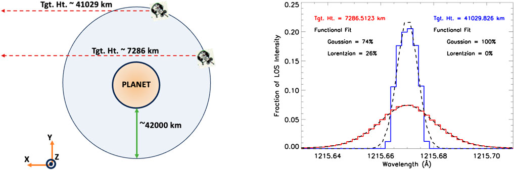
Figure 1. This figure demonstrates the changing width of the H Lyman α line with altitude for the GOES satellite lines of sight at different orbital positions. The planet here is Earth. The LOS tangent altitude of the spacecraft changes from ∼7,300 km to 41,000 km as it continuously points towards the Sun as shown in the left figure. The resulting calculated velocity distribution of the column of particles along the LOSs is shown on the right. The Y-axis represents the ratio of the particles in each velocity bin to the total number of particles along the LOS column integrated over all velocity bins.

Figure 2

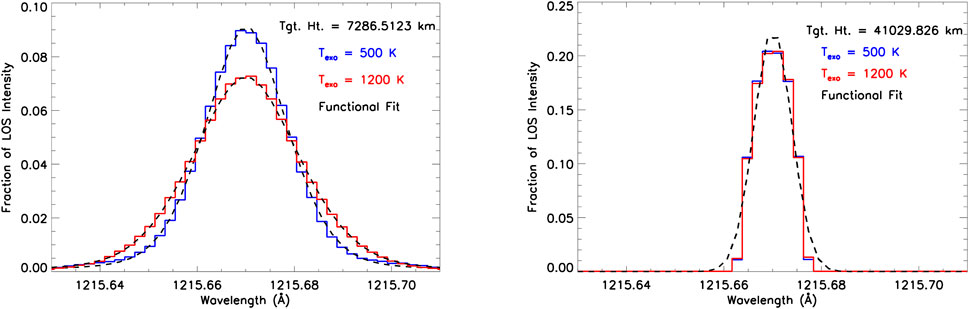
Figure 2. The shape of the H Lyman α line as a function of temperature and altitude for the GOES satellite lines of sight at different orbital positions. The planet here is Earth. The LOS tangent altitude of the spacecraft changes from ∼7,000 km to 41,000 km as it continuously points towards the Sun (Figure 1 left).

Figure 3

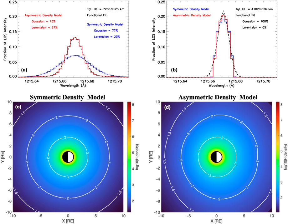
Figure 3. This figure demonstrates the effect of assuming a symmetric isothermal exosphere vs. an asymmetric non-isothermal exosphere driven by local temperature differences on the H Lyman α lineshape. The lines of sight are same as Figure 1. (a,b) show the spectral profile at lower and higher altitudes. Figure (c,d) show the H density distribution for the symmetric and the asymmetric case. The effect is more prominent at lower altitudes closer to the exobase, which is consistent with previous results from Holmström (2006), Bhattacharyya et al. (2017), Bhattacharyya et al. (2020).

Figure 4

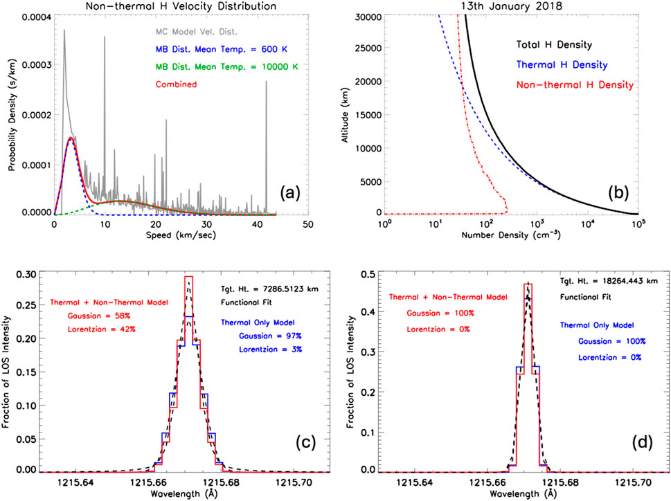
Figure 4. (a) The velocity distribution of the non-thermal H atoms in the exosphere of Mars determined via Monte Carlo (MC) modeling from HST observations, fitted with two Maxwellian distributions for modeling purposes. The grey curve represents the results of the MC model with the sharp peaks indicating statistical noise from the modeling process (b) The density distribution of the thermal and the non-thermal H determined from HST observations of the martian exosphere on 13 January 2018. Figures (a,b) are adapted from Bhattacharyya et al., (2023) (c) H Lyman α lineshape considering a thermal only model vs. a thermal + non-thermal model at a tangent altitude of ∼7,300 km. More contribution from the Lorentzian function is required to fit the thermal + non-thermal profile signifying the presence of non-thermal H along the column. (d) H Lyman α lineshape considering a thermal only model vs. a thermal + non-thermal model at a tangent altitude of ∼18,300 km. The LOS mimics the one shown in Figure 1 expect for the height of the tangent altitude. The column density of non-thermal H is too small to manifest itself as a detectable signal in the wings of the profile at higher altitudes.

3.1 Hydrogen Lyman α lineshape with altitude

The width of the H Lyman α line decreases with increasing radial distance from the planet. This effect is expected from the “evaporation and escape” theory of Chamberlain (1963). This theory considers only thermal H atoms on ballistic orbits, i.e., orbits bound to the parent object with their periapsis lying below the exobase, and escaping orbits, i.e., orbits that are not bound to the parent object or are hyperbolic in nature. The decrease in the line width with altitude happens as many of the atoms following ballistic orbits at the exobase do not have enough energy to reach the higher altitudes. The ratio of the number of atoms on ballistic to escaping orbits decreases with altitude. Figure 1 demonstrates the decreasing width of the H Lyman α line with altitude for the GOES satellite lines of sight which passes through Earth’s hydrogen exosphere. The exospheric characteristics assumed are symmetric and isothermal with an exobase temperature of 1000 K and an exobase H density of 1 × 10⁵ cm^-3 for the thermal H atoms. As seen in the figure, the wings of the line are more prominent at lower altitudes wherein the higher energy particles in escaping trajectories reside. The same wings disappear at higher altitudes for the narrower line as the higher energy particles now migrate towards the line center as more of their kinetic energy gets converted to potential energy lowering their velocities and the lower energy particles that formed the core of the line at lower altitudes are no longer available at higher altitudes. Due to the more prominent extended wings of the line at lower altitudes, a functional fit requires the application of both Gaussian core and Lorentzian wings to the line. At higher altitudes, the contribution from the Lorentzian wing disappears and a Gaussian functional fit to the line suffice.

3.2 Influence of temperature on the hydrogen Lyman α lineshape

Temperature is an important factor that influences the H Lyman α lineshape. Temperature here represents the mean temperature of the Maxwellian speed distribution of the hydrogen atoms at the exobase of the planet. The width of the Lyman α line is controlled by the mean temperature of the particles along an LOS column. A higher temperature results in a wider line whereas a lower temperature results in a narrower line. In general, the true shape of the H Lyman α line cannot be determined because of instrumental limitations. This is further discussed in Section 3.5. Figure 2 below shows the effect of temperature on the shape of the line at different LOS tangent altitudes. The LOSs considered here are the same as in Figure 1 for the GOES satellite. The parent planet is Earth, and the exosphere considered for the simulation is taken to be spherically symmetric and isothermal with an exobase H density of 1 × 10⁵ cm^-3 for the thermal H atoms. As can be seen in the figure, the difference in line width is more prominent at lower altitudes than at the higher altitudes. This is because at higher altitudes, the lower energy ballistic population present at the core of the line at lower altitudes has mostly dropped off and most particles which makes up the high-altitude line shape are in escaping orbits with energy distributions composed from the high energy tail of the Maxwellian velocity profile of the H atoms at the exobase. The wings of the line disappear at high altitudes as there are no particles left to populate those higher energy velocity bins anymore. The normalized lineshape becomes similar for both the 500 K and the 1200 K temperature because at these altitudes the lineshape is mostly composed of the high energy Maxwellian tail population which is basically the escaping population for both temperatures. Therefore, there is little difference in energy between them as all particles from the two temperature distributions are composed of energies greater than the gravitational potential of Earth. The column densities are also low at the high altitudes making is difficult to detect any wings in the lineshape.

3.3 Effect of assumptions about the exosphere inherent characteristics on the hydrogen Lyman α lineshape

Exospheres of terrestrial planets like Venus, Earth, and Mars are generally characterized by the well-established one-dimensional (1-D) Chamberlain theory (Chamberlain, 1963). This theory is based on the Liouville theorem wherein the time evolution of the distribution of particles along various trajectories remains a constant. This theory works well for exospheres which are considered to be almost collisionless due to the low number densities of particles in them. For most cases an isothermal and symmetric exosphere is considered. In such cases the only free parameters would be the exobase H number density and temperature which can then be used in the Chamberlain formulation to obtain the one-dimensional H number density distribution with altitude. Since most of the terrestrial planet exospheres are studied via remote sensing observations of the H Lyman α emission, which is optically thick, the 1-D assumption reduces the uncertainty in the modeling process. However, in reality exospheres of planets are neither isothermal nor symmetric (Bailey and Gruntman, 2011; Zoennchen et al., 2013, 2015, Chaffin et al., 2015; Bhattacharyya et al., 2020). One of the primary factors driving local asymmetries is temperature differences with solar zenith angle (SZA). The temperature difference between the sub-solar and anti-solar point have been found to be as high as 100 K for Mars (Bougher et al., 2015). These local temperature differences result in asymmetric distribution of the H atoms at altitudes close to the exobase. However, at higher altitudes, these differences become diluted with the density distribution approaching a symmetric structure. This happens due to the long time of flight of the H atoms (hours instead of minutes/seconds typical of heavier elements) (Clarke et al., 2014). Therefore, at higher altitudes a unit volume of space is likely to contain H atoms from different solar zenith angles and the average temperature of every unit volume approaches a constant value making it isothermal (Holmström, 2006; Bhattacharyya et al., 2017). This effect imprints itself on the velocity distribution of the H atoms which in-turn is manifested in the H Lyman α lineshape. Figure 3 below demonstrates this effect for the same two lines of sight for the GOES spacecraft at Earth. Here we have modeled the exospheric density distribution with a symmetric 1-D Chamberlain model for an exobase temperature of 1033 K and an exobase H density of 3.01 × 10⁵ cm^-3 for the thermal H atoms with background atmospheric conditions taken from NRLMSISE-00 for SZA = 0° for an arbitrary day, 16 November 2015 (Picone et al., 2002). The generation of the asymmetric density distribution follows the theoretical approach of Bhattacharyya et al. (2020), appendix A.1. This is a 2-D model which considers asymmetry brought on by the variation in temperature with SZA that has the largest effect on exospheric structure due to variations in local temperature. The asymmetric model sub-solar density and temperature value is the same as the symmetric model. The temperature variation with SZA is obtained from NRLMSISE-00 for the same day. The extension of the exobase density as a function of SZA is done using the relationship devised by Hodges and Johnson (1968) for light species: $n{T}^{5/2}=constant$. Here is $n$ is the exobase H density and $T$ is the exobase H temperature -. Knowing the resolved H at Lyman α lineshape will provide clues to the asymmetric nature of the exospheres of terrestrial solar system bodies. The symmetric and asymmetric density files are available at Bhattacharyya (2025).

3.4 Effect of the presence of non-thermal atoms on the hydrogen Lyman α lineshape

Non-thermal H atoms are ubiquitous in the exospheres of terrestrial planets. Both direct and indirect evidence of these H atoms has been observationally detected in the exospheres of Mars, Venus and Earth. At Mars, the exospheric temperature was found to be much higher (>400 K) than the thermospheric temperature (<380 K) for all seasons which led to the speculation that non-thermal atoms were present in the exosphere of Mars (Clarke et al., 2014; Chaffin et al., 2014; Bhattacharyya et al., 2015; Bougher et al., 2015). More recently, direct observational evidence was obtained for the presence of these atoms at Mars with the Hubble Space Telescope (Bhattacharyya et al., 2023). This direct evidence came in the form of changing scale height of the exosphere as it transitioned from being thermally dominated to non-thermally dominated. A similar effect was observed at Venus with the Venus Express orbiter (Chaufray et al., 2012). Such an effect was much easier to observe at Venus than at Mars due to the smaller gravity at Mars which increases the scale height of the thermal H atoms in its exosphere. The transition altitude where the exosphere becomes non-thermally dominated is around ∼20,000 km at Mars at aphelion whereas the same is <4,000 km at Venus. At Earth, too, indirect evidence for such atoms was determined during the analysis of Lyman α observations of the geocorona obtained by the Global Ultraviolet Imager (GUVI) onboard the Thermosphere Ionosphere Mesosphere Energetics and Dynamics (TIMED) mission (Qin and Waldrop, 2016). The reason for the lack of direct observational evidence of such atoms is mostly associated with the much smaller densities for these atoms in comparison to the thermal atoms, specifically at lower altitudes. Planet orbiting spacecrafts are also typically in low orbits like TIMED-GUVI, and MAVEN making it difficult to detect such populations through Lyman α observations.

One way to find direct evidence for such non-thermal atoms is by looking at the Lyman α emission lineshape at high resolution (>100,000) at low altitudes. This is because such atoms will likely manifest themselves in the wings of the line (high Doppler-shifted velocities) due to their much higher energies than the surrounding thermal H atoms which will be confined to the core of the Lyman α line. Figure 4 demonstrates this effect for Mars based on the density and energy distribution of non-thermal H atoms in the martian exosphere presented in Bhattacharyya et al., (2023). The calculation was done based on the energy and density distribution derived for the non-thermal H population at Mars for the HST observation of 13 January 2018. The energy distribution of the non-thermal population represented by the grey curve in Figure 4a was determined via Monte Carlo modeling (Bisikalo et al., 2018; Shematovich, 2013, 2021; Shematovich and Bisikalo, 2020, 2021). The Monte Carlo model can simulate secondary collisions between thermal H atoms present in the exosphere of Mars and energetic H atoms generated via charge exchange between martian exospheric thermal H and solar wind protons. At Mars the non-thermal population generated via such secondary collisions is found to match the HST observations of the martian H Lyman α emission at high altitudes and is now considered to be the primary source of non-thermal H at Mars (Bhattacharyya et al., 2023). A Maxwellian distribution was assumed for the two different non-thermal H population as demonstrated in panel (a) of Figure 4. This energetic population manifests itself in the wings of the Lyman α line resulting in more contribution from the wings which is demonstrated in the form of a larger contribution from the Lorentzian function for the thermal + non-thermal particle distribution profile. This effect is more evident at lower altitudes as the column of non-thermal H atoms is high enough to produce a detectable signal. One caveat of this calculation is the assumption of a Maxwellian distribution for the non-thermal atoms in the model. In reality, the non-thermal H atoms are likely to have a non-Maxwellian energy distribution with a higher detectable contribution at the wings of the line than the theoretical demonstration presented here. Currently, efforts are underway to make such a measurement at Earth with a high-resolution Spatial Heterodyne spectrograph (Harris et al., 2024) and a second instrument is being designed to operate in the FUV based on Fourier Transform Spectroscopy to measure the H Lyman α line at high resolution (De Oliveira et al., 2009; De Oliveira et al., 2011).

3.5 Effect of instrumental resolution on the measurement of the hydrogen Lyman α lineshape

The Sun is very bright in Lyman α (Milligan, 2021). This increases the visibility of all the neutral hydrogen present in the exospheres of certain terrestrial solar system objects like Venus, Earth, Mars, Titan and Pluto due to resonant scattering of the solar Lyman α photons. Knowing the detailed H Lyman α emission lineshape can reveal a lot about the exospheric properties of these objects, which, in turn, provides an important window into the dynamics of the object’s upper atmosphere. Most previous observations of the H Lyman α emission at such objects have consisted of broad-band imaging like HST observations of Mars (Clarke et al., 2014; Bhattacharyya et al., 2015) and imaging of the terrestrial H Lyman α emission with the Lyman Alpha Imaging Camera (LAICA) onboard the Japanese Aerospace Exploration Agency (JAXA) spacecraft, Proximate Object Close Flyby with Optical Navigation (PROCYON) (Kameda et al., 2017). Line-integrated photometric measurements were also done of the H Lyman α emission at Earth with NASA’s Two Wide-Angle Imaging Neutral-Atom Spectrometers (TWINS)/Lyman Alpha Detector (LAD) instrument (McComas et al., 2009). But the most common form of measurement is via low resolution spectrographs like TIMED-GUVI at Earth (Paxton et al., 2004), Mars Express-SPICAM and MAVEN-IUVS at Mars (Bertaux et al., 2006; McClintock et al., 2015), Venus Express-SPICAV (Bertaux et al., 2007) at Venus and Cassini Ultraviolet Imaging Spectrograph (UVIS) at Titan. These spectrographs had resolutions of R < 500 at Lyman α. Occasionally, higher resolution echelle spectrographs have been used to study the exosphere of Mars with HST’s Space Telescope Imaging Spectrograph (STIS) and with the MAVEN-IUVS instrument in Echelle mode. Even these high-resolution spectra had R < ∼25,000 at Lyman α. Therefore, none could be used to obtain information on the detailed structure of the H Lyman α emission line from the exospheres of these objects. The one measurement of the lineshape of the H Lyman α line at Earth was done with a hydrogen absorption cell onboard the OGO-5 spacecraft which revealed a measured exobase temperature of 1080 K, a value within the range of typical expected exobase temperatures at Earth (Bertaux, 1978). The data also indicated that the lineshape fit required the consideration of satellite particles distributed in a different manner than determined by the Chamberlain theory. To date no further measurements of such a kind have been attempted at any of the inner solar system planets.

Recent advances in UV instrumentation technology like higher efficiency gratings at shorter wavelengths have made it possible to design spectrographs with very high resolving powers of R ∼ 200,000–250,000. High resolving power provides unprecedented advantage towards deciphering the characteristics of the H atoms in the exosphere of planets. Specifically, it reduces the optical depth of the line in each wavelength bin presenting an optically thin rendition of otherwise a very optically thick line. This is because the column density of particles is restricted to particles with velocities only within the limits of the wavelength bin along a line of sight. This drastically reduces the photon scattering events along a line of sight and may make the column optically thin for certain wavelength bins depending on the resolution of the instrument and the exospheric number density of H atoms. Deciphering the characteristics of the H atoms by modeling an optically thick line can be done via radiative transfer modeling but results in much higher uncertainties in the derived density and energy distribution of the H atoms in the exospheres of terrestrial solar system objects (Bhattacharyya et al., 2017; Chaffin et al., 2018). An optically thin line has the advantage of the LOS intensity being directly proportional to the column density due to which a more precise density and energy distribution of the H atoms in the exospheres of objects may be determined without the use of complex radiative transfer models. A detailed high resolution structure on the wings of the H Lyman α line provides the advantage of detecting and characterizing the elusive non-thermal H atoms in the exosphere of planets even from low planet orbiting satellites, which otherwise requires global observations of the exosphere of a planet from large distances to detect the changing scale height of the atmosphere as it transitions from being thermal H dominated to non-thermal H dominated. Furthermore, if the instrument point spread function is smaller than the width of the measured line, then measuring the width of the observed lineshape will also provide information on the mean temperature of the column of H atoms, directly correlated to their energy distribution along a line of sight. Figure 5 demonstrates the advantage of a high-resolution instrument in terms of the optical depth of the measured line intensity for Earth. For R = 50,000, almost all of the Lyman α line is optically thick. For an R = 100,000, the core of the line is optically thick, but the wings start to become optically thin. For R > 150,000 the entire line becomes optically thin for all wavelength bins. The number of wavelength bins that may become optically thin for the resolved Lyman α line is dependent on the number density of H atoms present in the exosphere which are governed by lower atmospheric conditions, and space weather conditions along with instrument resolving power. The higher the resolving power of the instrument the more likely it is to render almost all of the wavelength bins optically thin at Lyman α for all exospheric conditions.

Figure 5

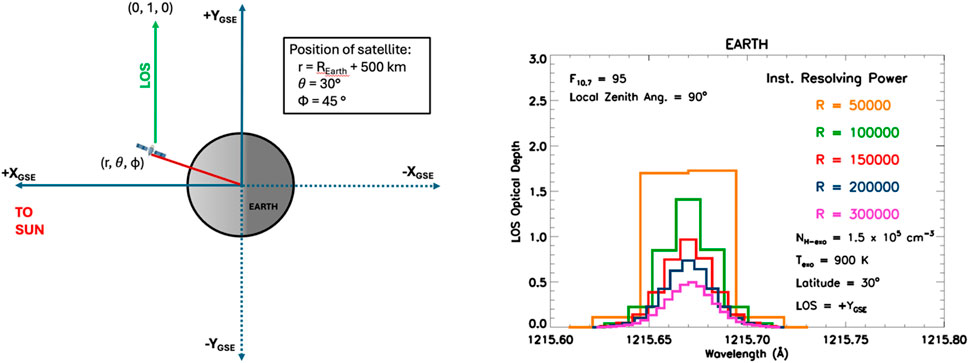
Figure 5. The figure on the left demonstrates an arbitrary line of sight along which the optical depth calculation was made for Earth. The figure on the right shows the decrease in the optical depth of the line with increasing resolving power of an instrument which can measure the H Lyman α line at Earth.

4 Discussion

This manuscript presents a detailed theoretical analysis of the hydrogen Lyman α lineshape applicable to the exospheres of terrestrial objects like Venus, Earth, Mars, Titan, and Pluto. The Lyman α line in these objects is optically thick and presently available observations mostly consist of low-resolution spectral measurements or broadband imaging of the H Lyman α line from which deriving the characteristics of the exospheric H atoms require complex radiative transfer modeling resulting in large uncertainties in the extracted density and energy distribution of the H atoms. Knowing the detailed Lyman α lineshape on the other hand may provide unprecedented information on the true nature of the H atoms present in the exospheres of many of the solar system terrestrial objects. Specifically, high resolution measurements of the Lyman α line allows for reduced optical depth rendering it optically thin in many of the velocity bins away from the line center even with low orbiting spacecrafts. This allows for a better estimation of the LOS density and energy distribution of the H atoms and makes the detection and characterization of non-thermal H atoms more obvious from wing intensity measurements. This high-energy population is otherwise elusive and difficult to characterize in most terrestrial solar system objects. At present, only one direct detection of such a population exists at Mars with HST broadband imaging from a large distance allowing for its characterization (Bhattacharyya et al., 2023). This theoretical study summarizes the information that can be obtained about the inherent properties of the exospheres of various terrestrial bodies with Lyman α line center optical depths 1 < τ < 500 with regards to the global structure and energy distribution of H atoms which is otherwise not possible from traditional low resolution or broad-band imaging measurements and highlights the need for developing technological capabilities to make such observations in the near future.

Data availability statement

Publicly available datasets were analyzed in this study. This data can be found here: https://mast.stsci.edu/search/ui/#/hst/results?proposal_id15097 and https://zenodo.org/records/8176255.

Author contributions

DB: Conceptualization, Investigation, Software, Writing – original draft. ET: Conceptualization, Writing – review and editing. JM: Funding acquisition, Writing – review and editing. GC-P: Investigation, Writing – review and editing. SC: Software, Writing – review and editing. WH: Investigation, Writing – review and editing. EM: Investigation, Writing – review and editing.

Funding

The author(s) declare that financial support was received for the research and/or publication of this article. This research was supported by the NOAA Earth Science from Operational Geostationary Satellite Systems grant NA20NES4400005-T1-01 to the University of Colorado, Boulder.

Conflict of interest

The authors declare that the research was conducted in the absence of any commercial or financial relationships that could be construed as a potential conflict of interest.

Generative AI statement

The author(s) declare that no Generative AI was used in the creation of this manuscript.

Publisher’s note

All claims expressed in this article are solely those of the authors and do not necessarily represent those of their affiliated organizations, or those of the publisher, the editors and the reviewers. Any product that may be evaluated in this article, or claim that may be made by its manufacturer, is not guaranteed or endorsed by the publisher.

References

Anderson, D. E., Meier, R. R., Hodges, R. R., and Tinsley, B. A. (1987). Hydrogen Balmer alpha intensity distributions and line profiles from multiple scattering theory using realistic geocoronal models. J. Geophys. Res. 92, 7619–7642. doi:10.1029/ja092ia07p07619

CrossRef Full Text | Google Scholar

Bailey, J., and Gruntman, M. (2011). Experimental study of exospheric hydrogen atom distributions by Lyman-alpha detectors on the TWINS mission. J. Geophys. Res. 116, A09302. doi:10.1029/2011ja016531

CrossRef Full Text | Google Scholar

Bertaux, J. L. (1978). Interpretation of OGO-5 line shape measurements of Lyman-α emission from terrestrial exospheric hydrogen. Planet. Sp. Sci. 26, 431–447. doi:10.1016/0032-0633(78)90065-x

CrossRef Full Text | Google Scholar

Bertaux, J. L., Korablev, O., Perrier, S., Quémerais, E., Montmessin, F., Leblanc, F., et al. (2006). SPICAM on Mars Express: observing modes and overview of UV spectrometer data and scientific results. J. Geophys. Res. 111. doi:10.1029/2006je002690

CrossRef Full Text | Google Scholar

Bertaux, J. L., Nevejans, D., Korablev, O., Villard, E., Quémerais, E., Neefs, E., et al. (2007). SPICAV on Venus Express: three spectrometers to study the global structure and composition of the Venus atmosphere. Planet. Space Sci. 55, 1673–1700. doi:10.1016/j.pss.2007.01.016

CrossRef Full Text | Google Scholar

Beth, A., Garnier, P., Toublanc, D., Dandouras, I., Mazelle, C., and Kotova, A. (2014). Modeling the satellite particle population in the planetary exospheres: application to Earth, Titan, and Mars. Icarus 227, 21–36. doi:10.1016/j.icarus.2013.07.031

CrossRef Full Text | Google Scholar

Bhattacharyya, D. (2025). Symmetric and Asymmetric Hydrogen exospheric densities from Chamberlain formulation for Ly-a lineshape calculation. Zenodo. [Data set]. doi:10.5281/zenodo.15448022

CrossRef Full Text | Google Scholar

Bhattacharyya, D., Chaufray, J., Mayyasi, M., Clarke, J., Stone, S., Yelle, R., et al. (2020). Two-dimensional model for the martian exosphere: applications to hydrogen and deuterium Lyman alpha observations. Icarus 339, 113573. doi:10.1016/j.icarus.2019.113573

CrossRef Full Text | Google Scholar

Bhattacharyya, D., Clarke, J. T., Bertaux, J.-L., Chaufray, J.-Y., and Mayyasi, M. (2015). A strong seasonal dependence in the martian hydrogen exosphere. Geophys. Res. Lett. 42, 8678–8685. doi:10.1002/2015gl065804

CrossRef Full Text | Google Scholar

Bhattacharyya, D., Clarke, J. T., Bertaux, J. L., Chaufray, J. Y., and Mayyasi, M. (2017). Analysis and modeling of remote observations of the martian hydrogen exosphere. Icarus 281, 264–280. doi:10.1016/j.icarus.2016.08.034

CrossRef Full Text | Google Scholar

Bhattacharyya, D., Clarke, J. T., Mayyasi, M., Shematovich, V., Bisikalo, D., Chaufray, J. Y., et al. (2023). Evidence of non-thermal hydrogen in the exosphere of Mars resulting in enhanced water loss. J. Geophys. Res. Planets 128, e2023JE007801. doi:10.1029/2023je007801

CrossRef Full Text | Google Scholar

Bisikalo, D., Shematovich, V., Gerard, J.-C., and Hubert, B. (2018). Monte Carlo simulations of the interaction of fast proton and hydrogen atoms with the Martian atmosphere and comparison with in-situ measurements. JGR Space Phys. 123 (7), 5850–5861. doi:10.1029/2018ja025400

CrossRef Full Text | Google Scholar

Bougher, S., Pawlowski, D., Bell, J., Nelli, S., McDunn, T., Murphy, J., et al. (2015). Mars Global Ionosphere-Thermosphere Model: solar cycle, seasonal, and diurnal variations of the Mars upper atmosphere. J. Geophys. Res. Planets 120, 311–342. doi:10.1002/2014je004715

CrossRef Full Text | Google Scholar

Broadfoot, A. L., Sandel, B., Shemansky, D., Atreya, S., Donahue, T., Moos, H., et al. (1977). Ultraviolet spectrometer experiment for the Voyager mission. Space Sci. Rev. 21, 183. doi:10.1007/bf00200850

CrossRef Full Text | Google Scholar

Carberry Mogan, S. R., Tucker, O. J., Johnson, R. E., Roth, L., Alday, J., Vorburger, A., et al. (2022). Callisto’s atmosphere: first evidence for H₂ and constraints on H₂O. J. Geophys. Res. Planets 127. doi:10.1029/2022JE007294

CrossRef Full Text | Google Scholar

Chaffin, M., Chaufray, J. Y., Deighan, J., Schneider, N. M., Mayyasi, M., Clarke, J. T., et al. (2018). Mars H escape rates derived from MAVEN/IUVS Lyman alpha brightness measurements and their dependence on model assumptions. J. Geophys. Res. 123, 2192–2210. doi:10.1029/2018JE005574

CrossRef Full Text | Google Scholar

Chaffin, M. S., Chaufray, J. Y., Deighan, J., Schneider, N. M., McClintock, W. E., Stewart, A. I. F., et al. (2015). Three-dimensional structure in the Mars H corona revealed by IUVS on MAVEN. Geophys. Res. Lett. 42, 9001–9008. doi:10.1002/2015gl065287

CrossRef Full Text | Google Scholar

Chaffin, M. S., Chaufray, J. Y., Stewart, I., Montmessin, F., Schneider, N. M., and Bertaux, J. L. (2014). Unexpected variability of martian hydrogen escape. Geophys. Res. Lett. 41, 314–320. doi:10.1002/2013gl058578

CrossRef Full Text | Google Scholar

Chamberlain, J. W. (1963). Planetary coronae and atmospheric evaporation. Planet. & Space Sci. 8, 901–960. doi:10.1016/0032-0633(63)90122-3

CrossRef Full Text | Google Scholar

Chaufray, J. Y., Bertaux, J. L., LeBlanc, F., and Quemerais, E. (2008). Observation of the hydrogen corona with SPICAM on Mars express. Icarus 195, 598–613. doi:10.1016/j.icarus.2008.01.009

CrossRef Full Text | Google Scholar

Chaufray, J.-Y., Bertaux, J.-L., Quemerais, E., Villard, E., and Leblanc, F. (2012). Hydrogen density in the dayside Venusian exosphere derived from Lyman-alpha observations by SPICAV on Venus Express. Icarus 217, 767–778. doi:10.1016/j.icarus.2011.09.027

CrossRef Full Text | Google Scholar

Clarke, J. T., Bertaux, J.-L., Chaufray, J.-Y., Gladstone, G., Quemerais, E., Wilson, J., et al. (2014). A rapid decrease of the hydrogen corona of Mars. Geophys. Res. Lett. 41, 8013–8020. doi:10.1002/2014gl061803

CrossRef Full Text | Google Scholar

Clarke, J. T., Mayyasi, M., Bhattacharyya, D., Chaufray, J. Y., Schneider, N., Jakosky, B., et al. (2024). Martian atmospheric hydrogen and deuterium: seasonal changes and paradigm for escape to space. Sci. Adv 10, eadm7499. doi:10.1126/sciadv.adm7499

PubMed Abstract | CrossRef Full Text | Google Scholar

Clarke, J. T., Mayyasi, M., Bhattacharyya, D., Schneider, N. M., McClintock, W. E., Deighan, J. I., et al. (2017). Variability of D and H in the martian upper atmosphere observed with the MAVEN IUVS echelle channel. J. Geophys. Res. Space Phys. 122, 2336–2344. doi:10.1002/2016ja023479

CrossRef Full Text | Google Scholar

Clarke, J. T., Nichols, J., Gérard, J., Grodent, D., Hansen, K. C., Kurth, W., et al. (2009). Response of Jupiter’s and Saturn’s auroral activity to the solar wind. J. Geophys. Res. 114, A05210. doi:10.1029/2008JA013694

CrossRef Full Text | Google Scholar

De Oliveira, N., Joyeux, D., Phalippou, D., Rodier, J. C., Polack, F., Vervloet, M., et al. (2009). A Fourier transform spectrometer without a beam splitter for the vacuum ultraviolet range: from the optical design to the first UV spectrum. Rev. Sci. Instrum. 80 (4), 043101. doi:10.1063/1.3111452

PubMed Abstract | CrossRef Full Text | Google Scholar

De Oliveira, N., Roudjane, M., Joyeux, D., Phalippou, D., Rodier, J. C., and Nahon, L. (2011). High-resolution broad-bandwidth Fourier-transform absorption spectroscopy in the VUV range down to 40 nm. Nat. Photonics 5 (3), 149–153. doi:10.1038/nphoton.2010.314

CrossRef Full Text | Google Scholar

Gardner, D. D., Mierkiewicz, E. J., Roesler, S., Nossal, S. M., and Haffner, L. M. (2017). Constraining Balmer alpha fine structure excitation measured in geocoronal hydrogen observations. J. Geophys. Res. Space Phys. 122 (10), 727–10. doi:10.1002/2017ja024055

CrossRef Full Text | Google Scholar

Harris, W. M., Corliss, J. B., Maciel, R., Mierkiewicz, E., Bhattacharyya, D., and Cucho-Padin, G. (2024). Investigation of the energetic and radiative transfer properties of exospheric hydrogen with the Hydrogen Emission Line Interferometric eXplorer (HELIX), 13093. SPIE, 155–165.

Google Scholar

Hedelt, P., Ito, Y., Keller, H., Reulke, R., Wurz, P., Lammer, H., et al. (2010). Titan’s atomic hydrogen corona. Icarus 210, 424–435. doi:10.1016/j.icarus.2010.06.012

CrossRef Full Text | Google Scholar

Hodges, R. R. (1994). Monte Carlo simulation of the terrestrial hydrogen exosphere. J. Geophys. Res. 99 (12), 23229–23247. doi:10.1029/94JA02183

CrossRef Full Text | Google Scholar

Hodges, R. R., and Johnson, F. S. (1968). Lateral transport in planetary exospheres. J. Geophys. Res. 73, 7307–7317. doi:10.1029/ja073i023p07307

CrossRef Full Text | Google Scholar

Holmström, M. (2006). Asymmetries in Mars’ exosphere. Implications for X-ray and ENA imaging. Space Sci. Rev. 126, 435–445. doi:10.1007/s11214-006-9036-7

CrossRef Full Text | Google Scholar

Hunten, D. M., and McElroy, M. B. (1970). Production and escape of hydrogen on Mars. J. Geophys. Res. 75, 5989–6001. doi:10.1029/ja075i031p05989

CrossRef Full Text | Google Scholar

Hunten, D. M., and Strobel, D. F. (1974). Production and escape of terrestrial hydrogen. J. Atmos. Sci. 31, 305–317. doi:10.1175/1520-0469(1974)031<0305:paeoth>2.0.co;2

CrossRef Full Text | Google Scholar

Ilie, R., Skoug, R., Funsten, H. O., Liemohn, M. W., Bailey, J. J., and Gruntman, M. (2013). The impact of geocoronal density on ring current development. J. Atmos. Solar-Terrestrial Phys. 99, 92–103. doi:10.1016/j.jastp.2012.03.010

CrossRef Full Text | Google Scholar

Jakosky, B. M., Brain, D., Chaffin, M., Curry, S., Deighan, J., Grebowsky, J., et al. (2018). Loss of the martian atmosphere to space: present-day loss rates determined from MAVEN observations and integrated loss through time. Icarus 315, 146–157. doi:10.1016/j.icarus.2018.05.030

CrossRef Full Text | Google Scholar

Kameda, S., Ikezawa, S., Sato, M., Kuwabara, M., Osada, N., Murakami, G., et al. (2017). Ecliptic north-south symmetry of hydrogen geocorona. Geophys. Res. Lett. 44 (11), 706–711. doi:10.1002/2017GL075915

CrossRef Full Text | Google Scholar

Krall, J., Glocer, A., Fok, M.-C., Nossal, S. M., and Huba, J. D. (2018). The unknown hydrogen exosphere: space weather implications. Space weather. 16, 205–215. doi:10.1002/2017SW001780

CrossRef Full Text | Google Scholar

Krasnopolsky, V. A. (2008). High-resolution spectroscopy of Venus: detection of OCS, upper limit to H₂S, and latitudinal variations of CO and HF in the upper cloud layer. Icarus 197, 377–385. doi:10.1016/j.icarus.2008.05.020

CrossRef Full Text | Google Scholar

LeBlanc, F., Oza, A., Leclercq, L., Schmidt, C., Cassidy, T., Modolo, R., et al. (2017). On the orbital variability of Ganymede’s atmosphere. Icarus 293, 185–198. doi:10.1016/j.icarus.2017.04.025

CrossRef Full Text | Google Scholar

Machol, J. L., Thiemann, E., Bhattacharyya, D., Snow, M., Riley, A., Codrescu, S., et al. (2021). “Preliminary exospheric neutral hydrogen density retrievals from GOES-R EUV measurements above 3 RE,” in In AGU fall meeting 2021 (New Orleans, Louisiana: AGU).

Google Scholar

Marconi, M. L. (2007). A kinetic model of Ganymede’s atmosphere. Icarus 190 (1), 155–174. doi:10.1016/j.icarus.2007.02.016

CrossRef Full Text | Google Scholar

McClintock, W. E., Schneider, N. M., Holsclaw, G. M., Clarke, J. T., Hoskins, A. C., Stewart, I., et al. (2015). The imaging ultraviolet spectrograph (IUVS) for the MAVEN mission. Sp. Sci. Rev. 195, 75–124. doi:10.1007/s11214-014-0098-7

CrossRef Full Text | Google Scholar

McComas, D. J., Allegrini, F., Baldonado, J., Blake, B., Brandt, P. C., Burch, J., et al. (2009). The two wide-angle imaging neutral-atom spectrometers (TWINS) NASA mission-of-opportunity. Space Sci. Rev. 142 (1), 157–231. doi:10.1007/s11214-008-9467-4

CrossRef Full Text | Google Scholar

McElroy, M. B., and Donahue, T. M. (1972). Stability of the martian atmosphere. Science 177, 986–988. doi:10.1126/science.177.4053.986

PubMed Abstract | CrossRef Full Text | Google Scholar

Meier, R. R. (1991). Ultraviolet spectroscopy and remote sensing of the upper atmosphere. Space Sci. Rev. 58, 1–185. doi:10.1007/bf01206000

CrossRef Full Text | Google Scholar

Mierkiewicz, E. J., Roesler, F. L., and Nossal, S. M. (2012). Observed seasonal variations in exospheric effective temperatures. J. Geophys. Res. 117. doi:10.1029/2011JA017123

CrossRef Full Text | Google Scholar

Mierkiewicz, E. J., Roesler, F. L., Nossal, S. M., and Reynolds, R. J. (2006). Geocoronal hydrogen studies using Fabry-Perot interferometers, part1: instrumentation, observations, and analysis. J. Atm. And Sol. Terr. Phys. 68, 1520–1552. doi:10.1016/j.jastp.2005.08.024

CrossRef Full Text | Google Scholar

Milligan, R. O. (2021). Solar irradiance variability due to solar flares observed in Lyman-Alpha emission. Sol. Phys. 296, 51. doi:10.1007/s11207-021-01796-3

CrossRef Full Text | Google Scholar

Nossal, S. M., Mierkiewicz, E. J., Roesler, F. L., Haffner, L. M., Reynolds, R. J., and Woodward, R. C. (2008). Geocoronal hydrogen observations spanning three solar minima. J. Geophys. Res. 113. doi:10.1029/2008JA013380

CrossRef Full Text | Google Scholar

Nossal, S. M., Roesler, F. L., Mierkiewicz, E. J., and Reynolds, R. J. (2004). Observations of solar cyclical variations in geocoronal Hα column emission intensities. Geophys. Res. Lett. 31. doi:10.1029/2003GL018729

CrossRef Full Text | Google Scholar

Paxton, L. J., Christensen, A. B., Morrison, D., Wolven, B., Kil, H., Zhang, Y., et al. (2004). “GUVI: a hyperspectral imager for geospace,” in Instruments, science, and methods for geospace and planetary remote sensing. SPIE proceedings vo. Editors C. A. Nardell, P. G. Lucey, J.-H. Yee, and J. B. Garvin (SPIE Bellingham, WA), 5660, 228–240. doi:10.1117/12.579171

CrossRef Full Text | Google Scholar

Picone, J. M., Hedin, A. E., Drob, D. P., and Aikin, A. C. (2002). NRLMSISE-00 empirical model of the atmosphere: statistical comparisons and scientific issues. J. Geophys. Res. 107 (A12), 1468. doi:10.1029/2002JA009430

CrossRef Full Text | Google Scholar

Qin, J., and Waldrop, L. (2016). Non-thermal hydrogen atoms in the terrestrial upper thermosphere. Nat. Comm. 7, 13655. doi:10.1038/ncomms13655

PubMed Abstract | CrossRef Full Text | Google Scholar

Roth, L., Alday, J., Becker, T., Ivchenko, N., and Retherford, K. (2017). Detection of a hydrogen corona at Callisto. J. Geophys. Res. Planets 122, 1046–1055. doi:10.1002/2017je005294

CrossRef Full Text | Google Scholar

Roth, L., Marchesini, G., Becker, T. M., Hoeijmakers, H. J., Molyneux, P. M., Retherford, K. D., et al. (2023). Probing Ganymede’s atmosphere with HST Lyα images in transit of Jupiter. Planet. Sci. J. 4 (12), 12. doi:10.3847/PSJ/acaf7f

CrossRef Full Text | Google Scholar

Shematovich, V. (2013). Suprathermal oxygen and hydrogen atoms in the upper Martian atmosphere. Sol. Syst. Res. 47 (6), 437–445. doi:10.1134/s0038094613060087

CrossRef Full Text | Google Scholar

Shematovich, V. (2021). Atmospheric loss of atomic oxygen during proton aurorae on Mars. Sol. Syst. Res. 55 (4), 324–334. doi:10.1134/s0038094621040079

CrossRef Full Text | Google Scholar

Shematovich, V., and Bisikalo, D. (2020). Kinetic calculations of the charge exchange efficiency for solar wind protons in the extended martian hydrogen corona. Astron. Rep. 64 (10), 863–869. doi:10.1134/s1063772920110074

CrossRef Full Text | Google Scholar

Shematovich, V., and Bisikalo, D. (2021). A kinetic model for precipitation of solar wind protons into the Martian atmosphere. Astron. Rep. 65 (9), 869–875. doi:10.1134/s106377292110036x

CrossRef Full Text | Google Scholar

Thiemann, E., Bhattacharyya, D., Machol, J., Snow, M., Allyssa, R., Codrescu, S., et al. (2021). “A window into the optically thick hydrogen geocorona from GOES-R solar occultations,” in In AGU fall meeting 2021 (New Orleans, Louisiana: AGU).

Google Scholar

Vidal-Madjar, A., and Bertaux, J. L. (1972). A calculated hydrogen distribution in the exosphere. Planet. & Sp. Sci. 20, 1147–1162. doi:10.1016/0032-0633(72)90004-9

CrossRef Full Text | Google Scholar

Yung, Y. L., and Demore, W. B. (1982). Photochemistry of the stratosphere of Venus: implications for atmospheric evolution. Icarus 51, 199–247. doi:10.1016/0019-1035(82)90080-x

CrossRef Full Text | Google Scholar

Zoennchen, J. H., Nass, U., and Fahr, H. J. (2013). Exospheric hydrogen density distributions for equinox and summer solstice observed with TWINS1/2 during solar minimum. Ann. Geophys. 31, 513–527. doi:10.5194/angeo-31-513-2013

CrossRef Full Text | Google Scholar

Zoennchen, J. H., Nass, U., and Fahr, H. J. (2015). Terrestrial exospheric hydrogen density distributions under solar minimum and solar maximum conditions observed by the TWINS stereo mission. Ann. Geophys. 33 (3), 413–426. doi:10.5194/angeo-33-413-2015

CrossRef Full Text | Google Scholar